The Multiplicity Function of Galaxies

The multiplicity function (MF) of groups and clusters of galaxies is determined using galaxy catalogues extracted from a set of Digitized Palomar Sky Survey (DPOSS) plates. The two different types of structures (of low and high richness) were identified using two different algorithms: a modified version of the van Albada method for groups, and a peak finding algorithm for larger structures. In a $300deg^{2}$ area up to $z<0.2$, we find 2944 groups and 179 clusters. Our MF covers a wide range of richnesses, from 2 to 200, and the two MF’s derived by the two algorithms match smoothly without the need for additional conditions or normalisations. The resulting multiplicity function, of slope $\alpha=-2.08\pm 0.07$, strongly resembles a power law.

1 Introduction

The multiplicity function (hereafter MF), in its differential form, is defined as the number of groups or clusters per area or volume unit and per richness unit.
The MF, which is the richness spectrum of galaxy aggregates, parametrises the observed clustering of galaxies and hence, together with the correlation and luminosity functions, is one of the fundamental cosmological observables. With respect to the complete description of clustering, the MF is complementary to the covariance function (which is related to the two-point correlation function), being related to the ratio of the amplitude of the higher-order to the two-point correlation functions (Gott & Turner, 1977, hereafter GT). Due to computational costs and errors, the measurement of correlation functions of order $N$ becomes unreliable for $N>3$, and the MF is therefore a crucial means of obtaining information on higher order clustering.
The Press–Schechter theory (Press & Schecter, 1974) states that the shape of the mass function (a power-law mass distribution with an exponential cutoff at the bright end) should provide important clues concerning the conditions at the epoch of recombination and does not depend on the cosmic density parameter $\Omega$. The steepness of the initial density fluctuation spectrum constrains the broadness of the mass function.
The MF, the mass function or the luminosity function all describe in a similar way the cosmic abundance of objects and, in fact, present similar shape (Bachall, 1979).

Despite the fact that the early descriptions of galaxy clustering properties were given in terms of the MF (Gott & Turner, 1977), most authors have focused on the shape of the mass function, which can be directly compared to the PS formalism. Even when the observed quantity is the MF, some authors (Bachall & Cen, 1993) prefer to convert it into a mass function using a reliable M/L ratio. Nevertheless, one must consider all of the uncertainties introduced by the mass estimation, which are propagated to the mass function determination. These include errors in the internal velocity dispersion used for dynamical mass estimates, the large intrinsic scatter in the richness-mass relation, and errors in assuming dynamical equilibrium for all clusters when using X-ray data (Girardi et al., 1998).

The main problem which must be overcome when determining the MF is the production of a statistically significant and unbiased catalogue of groups and clusters covering a large enough area of the sky and encompassing cosmic structures spanning a wide range of richness, from very low multiplicity structures such as galaxy triplets, up to very rich clusters with several hundred members.

In the past, catalogues of groups and clusters have been derived from either 3-D data (cf. Maia et al., 1989; Ramella et al., 1989, 2001, 2002), or from projected (2-D) data (de Vaucouleurs, 1975a, b; Turner & Gott, 1976; Materne, 1978; de Filippis et al., 2000). All these catalogues are derived from different data sets and with different algorithms and are therefore affected by different biases favouring the detection of structures in a given richness range; biases induced by the topology of the data, by the limited size of the survey, by ambiguities in the selection criteria, etc. Shectman (1985) pioneered the field of automated cluster finding in optical surveys using peak-finding methods, which has been refined and modified in many later projects (Maddox et al., 1990; Dalton et al., 1992; Lumsden et al., 1992; Nichol et al., 2001a; Gal et al., 2002). Based on a model dependent approach, Postman et al. (1996) developed the matched filter technique, which has been widely used, with several variants (Kawasaki et al., 1998; Schuecker & Bohringer, 1998; Lobo et al., 2000), including the adaptive matched filter (Kepner et al., 1999). In addition, the availability of multiband high accuracy CCD data, allowed the implementation of several cluster-finding methods based on the use of galaxy colours (Gladders & Yee, 2000; Goto et al., 2002; Nichol et al., 2001b; Andreon, 2003). An independent approach relied on the Voronoi tessellation technique as a peak finder (Ramella et al., 2001; Kim et al., 2000) and a modified version, taking into account colours was implemented by Kim et al. (2002). More recently, other, more advanced pattern recognition tools such as Bayesian clustering (Murtagh et al., 2002), maximum likelihood (Cocco & Scaramella, 1999), and neural networks (Frattale Mascioli, Priv. Comm.) have been introduced.

Much less work has been done to detect poorer structures such as loose groups; two principal methods (and their successive elaborations) have been adopted. Turner & Gott (1976) presented the first tentative objective identification of groups as enhancements above a reliable threshold in the projected galaxy distribution. The ”Friends Of Friends” algorithm of Huchra & Geller (1982) generates a measure of correlation among galaxies and their neighbours, basing on their separation in the full 3-D space. A noticeable exception to the lack of low-richness catalogs has been the detection of compact groups, where several teams (de Carvalho & Djorgovski, 1995; Iovino et al., 1999, 2002) have proposed different approaches to their detection. For the determination of the MF, it is important to note that its derivation from the above cited catalogues is hindered by the fact that all of the above algorithms are optimised for the detection of either groups or clusters, and no systematic work has been done in matching their outcomes in the transition region between structures of low and high richness.

Here, we attempt the derivation of an accurate MF, starting from the galaxy catalogues extracted from DPOSS material.

The paper is structured as follows. In Sect. 2 we shortly summarise the properties of the Digitized Palomar Sky Survey (DPOSS) data (Djorgovski et al., 1998, 1999; Reid et al., 1991) used to derive the multiplicity function described in Sect. 5. In Sect. 3 we describe the algorithms used to detect groups (Sect. 3.1) and clusters (Sect. 3.2), while in Sect. 4 we discuss the simulations performed in order to evaluate the accuracy of the method, expressed in terms of completeness and fraction of spurious detections, and to evaluate the possible existence of systematic errors in the ranges of overlapping richness for the group and cluster finding procedures. Finally, in Sect. 6, we draw our conclusions. Through this paper we assume $H_{0}=100$ $km$ $s^{-1}Mpc^{-1}$.

2 The data

The data used in this paper were extracted from the DPOSS photographic plates (Djorgovski et al., 1998, 1999; Reid et al., 1991) using the SKICAT package (Weir et al., 1995a) which provides photometric, morphological and astrometric data for each detected object. SKICAT also provides a classification (Star/Galaxy) based on a classification tree (Weir et al., 1995b).
In DPOSS, the three photometric bands ($J,F$ and $N$) are individually calibrated to the Gunn system (Thuan & Gunn, 1976; Wade et al., 1979) by means of accurate CCD photometry of objects of intermediate luminosity, (to take into account the nonlinear response of the plates), with preferential targetting of galaxies. From the DPOSS data covering the selected regions, we extract, for each individual object: RA, Dec, total magnitude which best approximates the asymptotic magnitudes and the object classification.

DPOSS individual plate catalogues must be cleaned of spurious objects and artifacts (such as multiple detections coming from extended patchy objects, halos of bright stars, satellite tracks, etc.). In order to do so, we mask plate regions occupied by bright, extended and saturated objects which locally make object detection extremely unreliable. Subsequently, we matched catalogues obtained in each of the three photometric bands, by using the plate astrometric solution and by matching each object in one filter with the nearest objects in the two other filters (with a tolerance box of 7 arcsec, see Paolillo et al., 2001). Due to the different S/N ratios in the three bands, many objects had discordant star/galaxy classifications in catalogues obtained in the different bands. The number of such objects obviously increases at faint magnitudes (it needs to be stressed, however, that this problem is greatly reduced when a new training set for the classification is adopted, see Odewahn et al. (2002) for details). In order to exclude from our final catalogues the smallest number of true galaxies, we discard only the objects classified as stars in all three filters. Final catalogues were thus obtained for 10 DPOSS plates (see Tab. 1) covering a total area of $\sim 300$ sq. deg. spread at high galactic latitude ($\|b\|>30\deg$) (see Fig. 1), in order to reduce cosmic variance. Details on the photometric calibration of these particular plates can be found in Paolillo et al. (2001, 2003). We note that these calibrations are not the same as the general DPOSS calibrations described in Gal et al. (2002). Our catalogue of galaxies is limited in magnitude down to the Gunn $r=20.5mag$.

Table 1: List of DPOSS plates, from which we extracted our catalogues. Notes: (1) calibration from Paolillo et al. (2001); (2) calibration from Paolillo et al. (2003).

Plate	RA	Dec	Effective area
Num	(2000)	(2000)	($deg^{2}$)
610(1)	01:00	+15.0	30.0
680(1)	00:20	+10.0	37.8
682(1)	01:00	+10.0	38.7
688(1)	03:00	+10.0	38.5
693(1)	04:40	+10.0	30.2
752(1)	00:20	+05.0	32.0
755(1)	00:20	+05.0	24.3
757(1)	01:20	+05.0	24.6
827(2)	01:20	+00.0	10.1
829(1)	02:00	+00.0	24.6

Figure 1: Stereographic projection of a transequatorial sky region (ranging from $\delta=-5$ up to $20$ degs and from $R.A.=0$ up to $80$ degs) containing the ten selected DPOSS fields listed in Tab. 1. In order to trace the global investigated area, all the detected clusters (without any cut in magnitude) are represented.

3 Detection of galaxy overdensities (groups and clusters)

Making an arbitrary choice, we use the term ”groups” to denote those galaxy aggregates which consist of less than 20 objects, and ”clusters” for all richer structures. This definition is comparable to that of Abell (1958), but in our case we set an implicit threshold on the magnitude difference between the brightest and the faintest objects in the same structure, given by the limiting magnitude.

3.1 The procedure for groups

In order to detect galaxy associations of low richness ($N_{obj}<20$), we have implemented a modified version of van Albada’s algorithm originally developed for binary systems (see Oosterloo, 1989; Soares et al., 1995).

Taking into account only the position and the apparent magnitude for each galaxy in our catalog, we first search for the nearest neighbour in a given magnitude range, and then estimate the probability that the two objects are physically related.

For the fore/background galaxies, the projected distribution is assumed to be Poissonian and the probability that the angular separation between a given galaxy and its nearest neighbour falls in the range $\theta$ and $\theta+d\theta$, is:

$$P_{1}(\theta)d\theta=\exp\left[-\pi\theta^{2}\rho\right]2\pi\theta\rho d\theta$$ (1)

where $\rho$ is the surface density of background galaxies in the immediate neighbourhood. In order to combine the angular separations of different pairs into a single distribution, the quantity $x$ is defined as the ratio between the observed value of the distance ($\theta_{1}$) to the nearest neighbour and the expected theoretical mean value $<\theta_{1}>$ given by Eq. 1:

$$\theta_{1}\equiv x\left<\theta_{1}\right>=\frac{x}{2\sqrt{\rho}}$$ (2)

The resulting frequency distribution of $x$:

$$p_{1}(x)dx=\exp\left[-\frac{\pi x^{2}}{4}\right]\frac{\pi}{2}xdx$$ (3)

is then independent of the background density $\rho$.

The shape of the observed distribution, $p_{0}(x)$, and the Poisson distribution $p_{1}(x)$, for large $x$, are expected to be similar. If an excess is found in the observed distribution relative to the Poissonian expectation for small $x$ (see Fig. 2, lower panel), it is likely due to physical companions, which will tend to cluster at smaller distances than random projections.

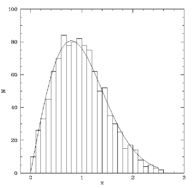
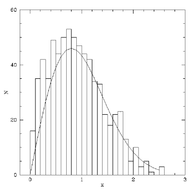
Figure 2: Upper panel: comparison of the Poissonian distribution (solid line) and the distribution of x’s (histogram) in a simulation with galaxies randomly distributed in the sky. Lower panel, as upper panel, but for actual observations: some of the nearest neighbours are physically linked (related) to the groups and produce an excess of neibourghs at small x.

Normalising the observed distribution to the Poisson distribution, we can use the excess $p_{0}(x)-p_{1}(x)$, observed at small $x$, to define the probability $p$ that two galaxies, located at a certain $x$, are physically associated:

$$p\equiv 1-\frac{p_{1}(x)}{p_{0}(x)}$$ (4)

In this formalism, all galaxy pairs having $p$ higher than a given threshold value are considered to be physical companions.

Iteration of the above procedure allows us to estimate the probability that other companions of higher order (up to N $\simeq$ 20) are physically related to the first object by comparing the observed distributions of higher order to the expected Poissonian distributions (normalised to the local density) for the second, third, etc. nearest neighbours ($p_{2}(x)$, $p_{3}(x)$, etc.).

Groups are then identified by associating all galaxies having probability $p$ higher than a given threshold value. Groups sharing one or more companions are finally merged into one single system. The total number of objects defines our richness for the groups.

To compute the quantity $x$ for every pair of galaxies, it is necessary to have an accurate estimate of the local galaxy density background $\rho$. To derive $\rho$, for each galaxy and within each magnitude interval, one first determines the distance to the $i$-th nearest neighbour $\theta_{i}$. The relation between $\theta_{i}$ and $\rho$ is given by the probability that the distance to the $i$-th nearest neighbour lies between $\theta$ and $\theta+d\theta$:

$$P_{i}(\theta)d\theta=\exp\left[-\pi\theta^{2}\rho\right]\frac{\left(\pi\theta^{2}\rho\right)^{i-1}}{\left(i-1\right)!}2\pi\theta\rho d\theta$$ (5)

The mean expected value of $\theta_{i}$ is:

$$\left<\theta_{i}\right>=\frac{\Gamma(i+0.5)}{[\left(i-1\right)!\sqrt{(}\pi\rho)]}$$ (6)

The higher the chosen value of $i$ (i.e. for large distances to the $i$-th neighbours), the lower the probability of being affected by possible physical companions, which would lead to an overestimate of the local background. Furthermore the width of the distribution of the ratio between $\theta_{i}$ and its mean value ($<\theta_{i}>$) decreases with increasing $i$. Thus if $i$ is large enough, it is possible to obtain an accurate estimate of $\rho$ from Eq. 6 by replacing the expected value $<\theta_{i}>$ with the observed one $\theta_{i}$. On the other hand, $i$ must not be too large, otherwise too much of the small scale clustering would be lost, and a large area of the plate will be affected by border effects (distant companions of galaxies located near the border of the plate will not follow a Poissonian statistics and will be preferentially located towards the center of the plate).
The choice of the value of $i$ is therefore a compromise that has to be made by taking into account all ofthe above factors.

3.2 The procedure of cluster identification

Candidate clusters were identified following a procedure similar to that of Shectman (1985). The catalogue of galaxies is binned into equal-area square bins in the sky, generating a two dimensional map (density map) of the number density of galaxies. The bin size ($1.2\arcmin$) is chosen such that the mean number of galaxies per bin is $\sim 1$, in order not to degrade the spatial resolution. The resulting map (Fig. 3) exhibits irregular structures corresponding to the presence of overdensities emerging above the intrinsic fluctuations of the background distribution.

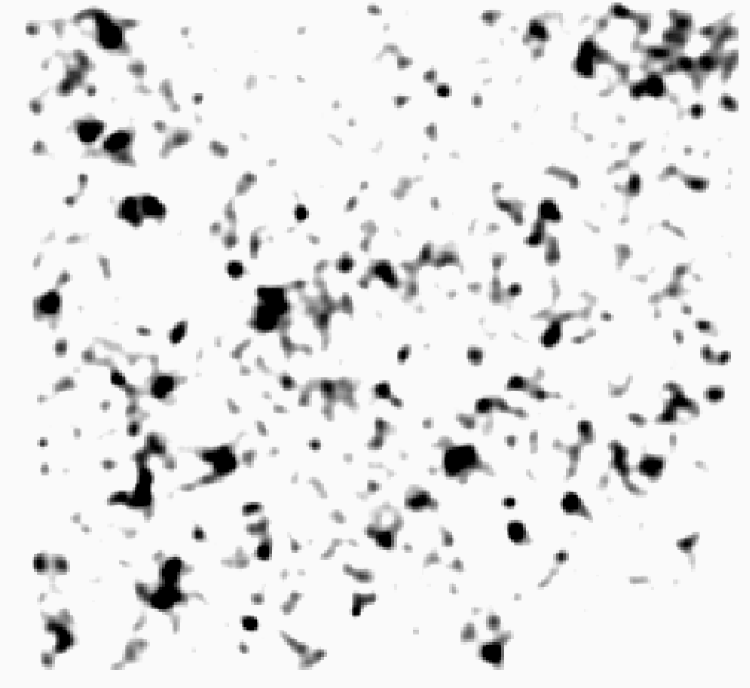
Figure 3: The smoothed two dimensional density map of the number density of galaxies for a field $5^{\circ}$ x $5^{\circ}$ centered at $RA=1h$ and $Dec=+15^{\circ}$ (DPOSS plate n. 610). The smoothing has been performed by a Gaussian 2-D filter with width ($\sim 3\arcmin$) typical for a cluster core at redshift $0.1-0.2$.

The large fluctuations existing in the distribution of background galaxies are due to the non-uniform background galaxy distribution. Once the density map has been created, the analysis of these maps poses similar problems to those of classical photometry, so we use S-Extractor (Bertin & Arnouts, 1996) for the detection of areas showing enhanced signal. S-Extractor is run on the density map searching for objects with a minimum detection area of 4 pixels above a global threshold of $0.4$ times the Poissonian background noise estimated from each plate using a background map. The evaluation of such background is a crucial step, strongly affecting the final richness estimate. The use of S-Extractor poses several problems (which cannot be trivially solved) since it is optimised to work on images with Gaussian statistics, while in density maps there are too few objects per bin, and they are distributed according to Poissonian statistics, thus making the background determination provided by S-Extractor unreliable. To circumvent this problem, we were forced to derive the background map in an alternative way. We first divide the original density map into sub-images of $\sim 1^{\circ}\times 1^{\circ}$, and then compute the Poissonian mean in each box, subsequently performing a fit with a 2-dimensional polynomial function of first order. We found a mean background density of 1640 per sq.deg. with a $\sigma$ of 148 galaxies. In this way, we remove those spatial frequencies higher (the clusters) than the mesh scale length. At the estimated typical redshift in our sample ($z=0.1-0.2$) this scale corresponds to a linear dimension of 9-15 Mpc. This map was then subtracted from the global frame before running the detection procedure.

The resulting density map was then smoothed in the detection step using S-Extractor with a Gaussian 2-D filter in order to match the cluster density profiles and, since we are searching structures with almost a Gaussian core, the filter width was chosen depending on the expected average apparent size for the cores ($\sim$ 250 kpc) of clusters in the redshift range ($z=0.1-0.2$) probed by our data. We stress that the choice of the otimal parameters strongly depends on the characteristics of the specific data sets and needs to be tuned on the simulations reproducing the behaviour of true catalogues.

The extracted parameters characterizing the detected overdensities are the density centroid in absolute equatorial coordinates (J2000), the isophotal area above the threshold, the S/N ratio of detection, and the number of objects inside the isophotal area, which we use to derive (after the background correction) our richness parameter for the clusters.

4 Outlines of the simulation

In order to test the limits of our group and cluster detection procedures, we performed simulations over a region having the same area and the galaxy counts as one POSS-II plate. In this way we could estimate the shortcomings of our procedure, such as the percentage of spurious detections and the percentage of lost objects; at the same time this helped in the fine tuning of the parameters of the detecting algorithms.

4.1 Simulation of the galaxy background

First we simulated the galaxy background assuming a uniform galaxy distribution. The number of simulated background galaxies is the average number of galaxies present in the DPOSS plates (approx $50000$ after excluding all the galaxies fainter than the limiting magnitude). To each background galaxy, a sky position, randomly extracted within the plate limits, and an apparent magnitude, distributed according to the observed galaxy counts, were assigned.

4.2 Simulation of galaxy groups

The number of groups to be simulated was extracted from the multiplicity function of Turner & Gott (1976).
We began by placing the principal galaxy of each group at random positions inside each field. Then, to each principal galaxy we assign an absolute magnitude and a redshift. Absolute magnitudes were extracted from a Schechter function with $\mathrm{M^{*}}=-19.80$ and $\mathrm{\alpha}=-1.25$ (Ramella et al., 1999), while the redshifts were assigned from the galaxy distribution observed in the Las Campanas redshift survey (Shectman et al., 1996). To each principal galaxy we then associate a number of secondary galaxies matching the multiplicity function mentioned above, each of these galaxies having the redshift of the corresponding principal galaxy. Taking into account the estimates provided in the literature, each simulated group was given a maximum standard dimension depending on its richness: a maximum radius of $0.26\ \mathrm{Mpc}$ for groups with $N_{obj}\leq 18$ members, while a maximum radius of $0.55\mathrm{Mpc}$ is used for groups with $N_{obj}>18$ members. All the secondary galaxies belonging to a group were then distributed inside the group volume, and each assigned an absolute magnitude generated from the same Schechter function as the brightest galaxies in the group. Finally, absolute magnitudes were re-transformed to apparent magnitudes by taking into account the cluster distance and the average $k$-corrections from Fukugita et al. (1995). The detection algorithm was then applied to the simulated plates in order to fine tune the algorithm parameters (threshold value of the probability $p$ and choice of the $i-{\rm th}$ nearest neighbour to compute the background galaxy density). The results of the simulations may be summarised as follows: the group detection algorithm loses 28% of the simulated groups and produces 43% spurious detections.
Fig. 4 shows that, in spite of the high contamination level, the MF shape is statistically preserved: the simulated MF (filled circles) and the detected MF (empty squares) differ on average by a vertical offset, which we take into account to correct the final group MF.

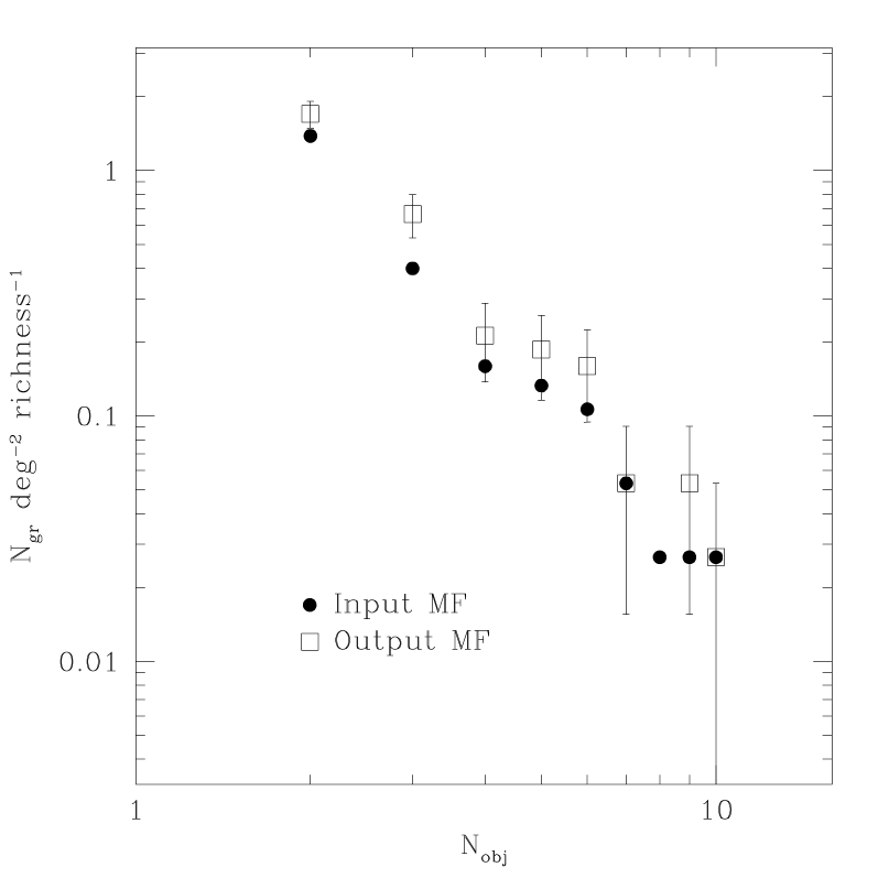
Figure 4: MF of simulated (filled circles) and detected (empty squares) groups. On the horizontal axis there is the number of galaxies in each group, that is the richness.

In Fig. 5 (left panel), we show, as an example, the outcome of one typical simulation. The centers of the simulated (dark dots) and detected (empty triangles) groups are plotted; a circle is drawn when the two match.

Figure 5: Simulated (dots) and detected (triangles) structures. Left: groups. Right: clusters. Circles highlight simulated groups/clusters which have been detected.

4.3 Simulation of clusters

Cluster simulations were performed with same assumptions used for the groups, with some crucial differences. The number of simulated clusters of a given richness (ranging from 2 to 200 galaxies) in an area of 37.59 squared degrees (approximately the area of one DPOSS plate) was determined from a preliminary analysis performed on $10$ DPOSS plates. In a second step, a power law multiplicity function was used, with the slope taken from the preliminary multiplicity function. In this way we tried to take into account the total number of low richness objects, which could not be measured from our preliminary analysis.

The absolute magnitudes of the principal galaxies were extracted from a Gaussian distribution centered on $-22.99\pm 1.0\ \mathrm{mag}$ (Schneider et al., 1983), while those for the secondary galaxies were extracted from the luminosity function of Paolillo et al. (2001). To take into account the richness dependence of the cluster dimensions, we arbitrarily adopted a core radius ($\sigma$ of the Gaussian profile) of $0.5\ \mathrm{Mpc}$ for clusters with $\leq 30$ members, while a core radius of $1.0\ \mathrm{Mpc}$ was used for clusters with $>30$ members. Although these values may appear somewhat high, the adoption of smaller values for the core radius would only make the detection easier and therefore the whole procedure more reliable. As with the groups, the detection algorithm was applied to a large number of simulated plates to test the algorithm performance as a function of the properties of the objects to be detected.

In Fig. 6, we plot, for a typical simulated plate, the assigned richness vs. the assigned core radius of the simulated clusters (open circles) and mark with a cross the clusters retrieved by the algorithm. Clusters with a very shallow profile or which are poor are preferentially lost.

Figure 6: The richness vs. the core radius of the simulated clusters (open circles). The crosses mark each retrieved cluster.

The dependence of the algorithm efficiency on the richness is shown in Fig. 7, where we plot the number of simulated (continuous line) and retrieved (dash shaded area) clusters in the typical plate area. All but two of the clusters having $N_{obj}>35$ are retrieved. In the range of richness $25<N_{obj}<35$, 80% of the clusters are retrieved. Considering that a cluster belonging to the Abell richness class 0 ($30-49$ members in a range of two magnitudes) has $N_{obj}>30$ ($N_{obj}$ includes the cluster galaxies in a range of at least four magnitudes), we are complete up to $z=0.2$ at least for all the Abell richness classes. Fig. 7 also shows that spurious detections (dot shaded area) are absent in the richness range where the algorithm works with the highest efficiency, and occur only in the range where the group finder is to be used.

Figure 7: Cluster number in the one plate area is plotted as a function of estimated richness. The continuous histogram represents the number of clusters given in input to the simulation; the dash shaded histogram represents the retrieved clusters and the dot shaded histogram the spurious detections. The richness bin grows exponentially as $2^{n/2}$ (see Sect. 5).

As already mentioned, the estimate of clusters richness is given by the number of objects within the detection isophote (isodensity counts). We wish to stress that this definition of richness depends on the redshift of the detected structure. The quality of the richness estimate has been tested using our simulations. In Fig. 8, the points follows bisector of the diagram (a bit shifted towards the upper half part of the plot), with a scatter in richness of $\sim 10$ galaxies (which is consistent with the background fluctuations). The small shift indicates an understimation of the retrieved richnesses. We are comparing the number of the galaxies put in a synthetic circular aperture (the simulated) with the richness in the isodensity irregular countours, as it is measured in the real case: in this way some galaxies are missed. If we use circular apertures of the cluster size (which are known in the simulations but not in the actual observations), the shift disappears. Points in the lower right part of the plot are due to overlapping clusters, for which (in the absence of a deblending procedure) the richness will obviously be overestimated.

Figure 8: Richness of the simulated vs. the detected clusters. The errors are inversely proportional to the signal to noise ratio for the detection.

5 The conjoined groups/clusters multiplicity function

Fig. 9 summarizes our main results. We plot the MF, defined as the number of groups or clusters per unit area and per unit of estimated richness (the groups/clusters richness is defined respectively in Sect. 3.1 and Sect. 3.2). For the clusters, the bin grows exponentially as $2^{n/2}$, in order to keep the $S/N$ ratio almost constant along the richness axis. For the groups, the bin was instead set equal to 1. In order to exclude the structures detected in the redshift range where our magnitude limited catalogue is incomplete, only clusters and groups where the brightest galaxy has $m<16.5$ (in Gunn $r$) were selected. Assuming that brightest galaxies may be used as standard candles, our selection in magnitude implies that $z<0.2$.

The procedures described above were applied separately for groups and clusters, obtaining two different multiplicity functions (marked with different symbols in Fig. 9). These MFs appear to define a common relation, without the need for any offsets or normalisations. We emphasize that a minor correction for completeness was applied only to the last point of the clusters MF. To correct the group’s MF for contamination by spurious detections (see Sect. 4.2), a global shift derived from the simulations was also applied. Only the Poissonian statistical fluctuations have been taken into account in the error estimate. For the high richness clusters, the error on the richness estimate is negligible with respect to the bin width. The error becomes relevant only in the same richness range where incompleteness is also significant.

In Fig. 10 we compare our results with a MF extracted by us from the USGC catalog of groups (Ramella et al., 2002). We adopt the same representation scheme for the two data set. Normalisation to the same volume was applied to the USGC groups, assuming a uniform distribution of objects in redshift both for our sample and the USGC sample. It is important to note that the two catalogs were derived in totally different ways. The USGC is generated using spectroscopic redshifts by a percolation method implemented by Ramella et al. (1997) for group detection, which is designed to reduce the risk of false detections introduced by chance projections.

The agreement between these two MFs (see Fig. 10), derived under totally different assumptions and using independent data sets, is due to similar biases affecting the estimated richnesses for both samples. For low $N_{obj}$ structures (groups) the similarity is apparent; in both cases, the methods count individual objects fulfilling the respective membership criteria but with secondary members having magnitudes falling within similar (i.e. $\sim$ four magnitudes) ranges with respect to the primary galaxy. For the clusters, instead, the different depths sampled by the two data sets, when compared to the different limiting magnitudes of the samples themselves, indicates that both methods sample very similar intervals of the cluster’s luminosity function.

Figure 9: The multiplicity function for galaxy structures ranging from small groups (filled triangles) to rich clusters (filled circles). We remove clusters in the richness range where detection efficiency is low.

Figure 10: Overplot of the MF of USGC2 groups (empty circles) on the multiplicity functions obtained from the DPOSS data.

6 Summary and discussion

We have implemented two algorithms for the detection of galaxy associations, one for groups and one for clusters. The former is a modified version of van Albada’s procedure to detect galaxy pairs, while the latter the Shectman (1985) approach, which uses a peak-finding procedure on a density map obtained from the galaxy catalogue.

We evaluated the performance of these methods via extensive simulations, which show that the group algorithm is reliable up to richness $20$, and the cluster algorithm is reliable at richnesses above $20$ galaxies. The two algorithms were then applied to a $\simeq 300$ square degree field extracted from DPOSS data (see Sect. 2). The resulting MFs show a remarkable internal consistency from the two procedures which produce independent MFs for groups and clusters, matching with no need for normalisation. Additionally, the MF derived using our technique on the 3-D based catalogues of Ramella et al. (2002) agrees with the MF derived from the projected DPOSS data. The final combined MF is well fit by a power-law of slope $\alpha=-2.08\pm 0.07$. The correlation coefficient on the log-log scale is $-0.98$.

The data set we used to determine the MF samples a volume [$\sim 300deg^{2}$, $z<0.2$] which is slightly smaller than that explored by Bachall et al. (2002) [$\sim 400deg^{2}$, $z=0.1-0.2$]. The total number of detected structures for $N>10$ in the Bachall et al. (2002) and in our sample is respectively $\sim 300$ and $\sim 370$. In a forthcoming paper we shall analyze the cosmological implications of the derived MF.