Searching for Planetary Transits in the Field of Open Cluster NGC 6819 - I.

Abstract

We present results from our survey for planetary transits in the field of the intermediate age ($\sim$2.5 Gyr), metal-rich ([Fe/H]$\sim$+0.07) open cluster NGC 6819. We have obtained high-precision time-series photometry for over 38,000 stars in this field and have developed an effective matched-filter algorithm to search for photometric transits. This algorithm identified 8 candidate stars showing multiple transit-like events, plus 3 stars with single eclipses. On closer inspection, while most are shown to be low mass stellar binaries, some of these events could be due to brown dwarf companions. The data for one of the single-transit candidates indicates a minimum radius for the companion similar to that of HD 209458b.

1 Introduction

Following the discoveries of Hot Jupiter-type extra-solar planets, it was apparent that a photometric survey to detect these planets in transit was feasible from ground-based telescopes. This was confirmed by the detection of transits by HD 209458b by Charbonneau et al. (2000) and Henry et al. (2000). Such a survey has the potential to broaden the search for planets over a greater volume of space by monitoring stars at fainter magnitudes than are accessible to the spectroscopic radial velocity technique. The transit method enables us to probe far greater numbers of stars simultaneously and so obtain a statistically significant sample of planets in a comparatively short time. Discoveries can be used to determine the abundance of planets in a range of stellar environments, allowing us to investigate the relationship between planet formation and key properties; for example metallicity, age, stellar and radiation density. Follow-up observations of transiting planets can provide vital information on individual planets – their true masses, radii and orbital inclinations – crucial for testing theories of planetary structure. Once transit candidates are obtained from photometric surveys, these data combined with spectrographic observations will not only provide this information but will also distinguish planetary transits from grazing-incidence eclipses by stellar and brown dwarf companions. Follow-up observations are discussed in greater detail in Section 7.1.

From the radial velocity survey results, we know that approximately 1 percent of F–K-type solar neighbourhood stars harbour hot Jupiters (giant planets with periods of $\sim$2–6 days). The typical orbital separation (0.05 AU) for these planets implies that about 10% of them should exhibit transits if their orbital planes are randomly oriented with respect to the line of sight. Assuming that planetary orbits are distributed isotropically, we can expect there to be one transit for every 1000 stars. The detection probability is affected by factors such as the sampling rate of the observations, the efficiency of detection from the data and the fraction of late-type dwarfs in the sample. Correspondingly, transit surveys that monitor tens of thousands of stars simultaneously may expect to detect tens of planets. This requirement must then be balanced against the need to avoid fields so crowded that blending makes stars difficult to measure precisely.

Janes (1996) suggested that open clusters would make a good compromise for ground-based surveys. They provide large numbers of stars within a relatively small field with minimal blending. They also provide a distinct population of stars of known age and metallicity and allow us to probe stars in the environment where they formed. Additionally, these fields provide a separate population of background stars for comparison.

A number of groups are pursuing transit surveys using large (2–4m) telescopes with wide field, mosaic CCD cameras. Most notably, the explore project has used the CTIO-4m and the 3.6m CFHT to observe two Galactic plane fields in 2001 (Yee et al., 2002). These data have revealed 3 possible planetary transit candidates, and the team are in the process of obtaining radial velocity follow-up (Mallén-Ornelas et al., 2002). The ogle group have used their microlensing observations of Galactic disc stars to search for transits in the lightcurves of $\sim$52,000 stars, yielding 59 candidates so far (Udalski et al., 2002). Dreizler et al. (2002) obtained classification spectra for 16 of these stars, allowing them to estimate the radius of the primary and infer the radius of the companion. This analysis ruled out 14 candidates as having stellar-mass companions, while the companions of two objects were found to have radii similar to that of HD 209458b. Recently, Mochejska et al. (2002) have undertaken a survey of open clusters using the F. L. Whipple Observatory’s 1.2m telescope, discovering 47 new, low amplitude variables.

In 1999 we began a survey of three open clusters for planetary transits: NGC 6819, 7789 and 6940. The wide field of view of the Isaac Newton Telescope’s (INT) Wide Field Camera (WFC) is ideally suited to this task, and we were awarded a total of 3 bright runs of 10 nights each in June/July 1999 and September 2000 for these observations.

Open cluster NGC 6819 was observed during the first 19 of these nights and the results presented here stem from our analysis of these data. The basic parameters of this cluster are given in Table 1. Previous relevant work on this cluster was discussed in Street et al. (2002); most important is a recent study by Kalirai et al. (2001) which provided $B$ and $V$ magnitudes for large numbers of stars in this field.

Table 1: Basic data on NGC 6819. Data taken from Kalirai et al. (2001) and the simbad database.

RA (J2000.0)	19h 41m
Dec (J2000.0)	+40$\degr$11′
$l$	73$\degr$.97
$b$	+8$\degr$.48
Distance (pc)	2754 $\pm$ 305
Radius	$\sim$9.5′
Age (Gyr)	2.5
$[Fe/H]$	+0.07
$E(B-V)$	0.10

In the rest of this paper, Section 2 details these observations, and Sections 3 and 4 present the data reduction procedure. Section 5 discusses our transit-detection algorithm while our results are presented in Section 6. Finally we draw conclusions in Section 8.

2 Observations

We observed NGC 6819 on 19 nights during 1999 June 22–30 and 1999 July 22–31, using the 2.5m Isaac Newton Telescope, La Palma. The Wide Field Camera (WFC) employs four 2048$\times$4096 pixel EEV CCDs to image a $\sim$0.5$\degr\times$0.5$\degr$ field of view with a pixel scale of 0.33$\arcsec$ pix^-1. The gain and readout noise values for each CCD were taken from the Cambridge Astronomical Survey Unit webpage and are listed in Table 2.

Table 2: Gain and readout noise values for the four WFC CCDs, taken from the Cambridge Astronomical Survey Unit webpage.

CCD No.	Gain (e- ADU-1)	Readout noise (ADU)
1	3.12	7.9
2	3.19	6.4
3	2.96	8.3
4	2.22	8.3

Three open clusters, NGC 6819, 6940 and 7789, were observed in rotation during these two runs, taking pairs of 300s exposures through the Sloan r’ filter on each visit. The readout time of the WFC at the time required 160 sec of deadtime between exposures. No dithering was applied between exposures as we aimed to place each star as close to the same pixel each time as possible. In practise, the $x,y$ shifts between images were up to a few pixels. NGC 6819 was observed for $\sim 7-8$ hours each night, typically resulting in 16 – 25 frames per night or about 2 frames/hour. In total, 361, 384, 364 and 325 frames were obtained of this cluster for CCDs 1 – 4 respectively. The number of available frames varied due to unpredictable readout failures which could affect individual CCDs. The average gap between pairs of exposures was, at most, roughly an hour and we had good observing conditions on all nights. The field of view covered by the WFC is shown in Figure 1.

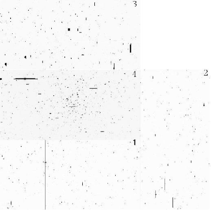
Figure 1: The WFC $\sim$0.5${}^{\degr}\times$0.5^° field of view covering open cluster NGC 6819; North is to the top of the image while East is to the left. The CCD numbers are given in the corners.

3 Data Reduction

We developed a semi-automated data reduction pipeline in order to process this large dataset. This pipeline has been previously described in Street et al. (2002) and in detail in Street (2002).

The debiasing, flatfielding and trimming of the frames were carried out using the Starlink package figaro Shortridge et al. (1998). A correction for the nonlinear response of each chip was also applied. Point-spread function (PSF) photometry was performed using iraf’s daophot task Stetson (1987). It was found that stars subtracted from an image using a fixed PSF showed residuals that varied with position. These residuals were best reduced by employing daophot’s “penny2” function and allowing it to vary quadratically with position. This is a two-component model, consisting of an elliptical Gaussian core and Lorentzian wings. Both parts of the model are aligned along separate and arbitrary position angles. daophot handles pixel defects, cosmic rays etc. by employing a formula which reduces the weights of pixels that do not converge towards the model as the fit is calculated. This is discussed in more detail in Davis (1994). The post-processing (discussed below) is also able to detect and remove strongly outlying points. Where a star of interest is found to lie close to dead columns/pixels conclusions have been drawn with caution. We chose to have the star positions re-fitted independently in each frame, having found that the cross-correlation technique aligned the star centroids to around $\sim 1$ pixel accuracy.

For a significant number of images, we found that a position-dependent element still remained in the magnitude residuals, particularly dominant along the long ($y$) axis of the CCD. To counteract this problem, we have employed our own post-processing software, described in Street et al. (2002). This included a procedure which cross-correlates all lightcurves in the sample in order to identify and remove remaining systematic trends.

Following this processing, the precision achieved is illustrated by plotting the RMS scatter in each star’s lightcurve against its weighted mean magnitude over the whole dataset. Figure 2 shows these plots for each CCD, and for reference shows the effects of the main expected sources of noise. While some systematic effects remain in the data, our software improves the precision particularly at brighter magnitudes, where we can achieve the $\sim$0.004 mag precision required to detect planetary transits. We notice that the residual systematic variations are reduced to a level of $\sim$0.0025–0.0035 mags. After post-processing, these residuals do not appear to show a positional distribution. We also notice that the “backbone” of points falls slightly below the theoretical noise prediction at the faint end. This seems to be due to daophot underestimating the magnitude errors used to weight the calculations at fainter magnitudes. We note the presence of “clumps” of stars with high RMS in CCD3. Investigation of these points reveals that they are hot pixels located in the vignetted areas and dead columns which this CCD suffers from.

(a) CCD 1

(b) CCD 2

(c) CCD 3

(d) CCD 4

Figure 2: The variation of RMS scatter in star lightcurves with magnitude for each of the four CCDs. Superimposed curves show the effects of various sources of noise.

Astrometric positions for all the stars in our sample were obtained using the method described in Street et al. (2002). The average RMS error in the resulting RA and Dec are presented in Table 3, and correspond to an RMS scatter of less than 1 pixel on the CCD.

Table 3: Average RMS error on RA and Dec positions in arcsec for each CCD.

CCD No.	$\delta$RA	$\delta$Dec
	(arcsec)	(arcsec)
1	0.118	0.110
2	0.232	0.363
3	0.289	0.294
4	0.172	0.180

4 Stellar Radii

4.1 Colour Index Calibration

Kalirai (2001) kindly provided us with $B-V$ colours indices for many of the stars in the NGC 6819 field. These data and the procedure used to cross-identify stars are described in Street et al. (2002). Although most of our data were taken in the Sloan r band, we obtained enough Sloan i data to calibrate approximate $V-R$ colours for all the stars in our sample in the following way. We calculated the mean broadband flux using known passband functions and the Bruzual, Persson, Gunn and Stryker atlas of stellar spectra. The mean broadband flux was then used to calculate theoretical magnitudes and colours for a range of stellar spectral types relative to the flux from Vega in that passband. The INT instrumental Sloan $r-i$ colours were calibrated by superimposing the xcal plot of Sloan $r-i$ against $B-V$ over that of the INT stars, and applying vertical and horizontal offsets. The horizontal offset provided the calibration factor for the INT data, in the sense that the true Sloan $r-i$ colour of a star ($r-i$) is found from the instrumental one ($r-i)_{inst}$ by adding the offset, $\Delta_{r-i}$:

$$r-i=(r-i)_{inst}+\Delta_{r-i}.$$ (1)

$\Delta_{r-i}$ was found to be 0$\aas@@fstack{m}$50, 0$\aas@@fstack{m}$50, 0$\aas@@fstack{m}$30 and 0$\aas@@fstack{m}$41 for the data from CCDs 1, 2, 3 and 4 respectively. In all cases, the vertical offset (the difference between the theoretical and measured $B-V$) was found to be 0$\aas@@fstack{m}$2. This we attribute to extinction in the direction of the cluster and is not very different from the value of $E(B-V)=0.1$ measured by Kalirai et al. (2001).

We used a similar method to convert the now-calibrated Sloan $r-i$ colours into Johnson $V-R$. xcal was used to produce a dataset of $V-R$ and corresponding Sloan $r-i$ values. To derive a formula to convert Sloan $r-i$ colours into Johnson $V-R$, a function was fitted to these data using the method of least squares. As the shape of the curve changes at $r-i\sim 0.4$, two functions were fitted; a straight line for $r-i$ values $\sim-0.2\sim 0.4$ and an exponential function for the remaining curve:

$$V-R=\begin{cases}0.009+0.93(r-i)&-0.2\leq r-i\leq 0.356\\ 1.30-1.72e^{-1.6(r-i)}&0.356\leq r-i\leq 2.5\end{cases}$$ (2)

These relations were then used to calculate $V-R$ colour indices for all INT stars with Sloan $r-i$ colours.

4.2 Colour-Magnitude Diagram

Figure 3 shows the $(V,V-R)$ colour-magnitude diagrams (CMD) for the four CCDs. The cluster main sequence is clearly visible in the data from CCD4 and faintly in the other three plots. This is expected from the radius of the cluster Kalirai et al. (2001) which fits within the field of view of one of the WFC CCDs. Field stars greatly outnumber cluster members in these data, and are located above and below the cluster main sequence in the CMD. The field stars above and below the cluster main sequence are predominantly main sequence stars at closer and more remote distances than the cluster, respectively. In our following analysis, we assume that all stars in our sample are main sequence. This is reasonable since class IV subgiants are sufficiently rare that their frequency in the sample is negligible. Giant stars are so bright ($-0\aas@@fstack{m}4<M_{V}<1\aas@@fstack{m}2$) that for one to be measurable (unsaturated) in our data it would have to be at a distance of $\geq$9 Kpc. We therefore adopt main sequence relationships and use the likely distance and spectral type and hence radius of the stars in our sample.

(a) CCD 1

(b) CCD 2

(c) CCD 3

(d) CCD 4

Figure 3: $V$.vs.$V-R$ colour-magnitude diagrams for the four WFC CCDs. The transit candidate stars are highlighted.

Figure 4: RMS scatter against $V-R$ colour for all $\sim$38,000 stars in our sample. The overlaid curves give the predicted transit depth for cluster member stars transited by planets of various radii.

4.3 Stellar Radii

We use the $V-R$ index to estimate the radius of each star in this survey. This was done by interpolating between measured values of $V-R$ and $R_{*}$ for the range of main sequence star types from Gray (1992). These values were supplemented at the low-mass end by data from Reid & Gizis (1997), who list $V-R$ index, absolute magnitude and spectral type for 106 low-mass systems. The absolute magnitudes were then used to calculate the radii of these stars. An exponential curve was least-squares fitted to the Reid and Gizis data and used to calculate values of stellar radii at fixed intervals of $V-R$ in order to provide one smooth, continuous dataset. Interpolation over this dataset was then used to compute main sequence star radii from the $V-R$ colour index of each star. Figure 4 plots RMS scatter versus $V-R$ colour. This is overlaid with curves illustrating the predicted transit depth of planets with radii of 0.5, 1.0 and 2.0 R_jup orbiting cluster member stars of various masses. If the RMS of a given star falls below one of these curves, then we would expect to be able to detect a transit of a planet that size around that star.

We find that $\sim$30% of the stars in our sample fall below the 1.0 R_jup -transit curve, while $\sim$79% fall below the 2.0 R_jup line. Thus around $\sim$11,500 and $\sim$30,000 stars, respectively, are measured to sufficient precision to allow the detection of transits. Assuming $\sim$1% of all main sequence stars have hot Jupiter companions and $\sim$10% of those transit, then we can roughly expect to detect $\sim$11 Jupiter-radius objects in our data.

5 Transit Detection Algorithm

Having obtained the required high-precision photometry, there are a number of different approaches to the problem of detecting transit events. We have developed our own transit-finding software, using the method of matched-filter analysis.

After identifying and removing known large-amplitude variables from the data, the software works in two stages. The first stage, or “standard search”, generates a series of model lightcurves with a single transit. These models are generated for a range of transit durations $0.5<\delta t<5.0$ hours, in intervals of 0.25 hours and with the time of mid-transit ranging from the start to the end of the observing campaign in steps of $\delta t/4$. A constant magnitude is least-squares-fitted to each lightcurve and the corresponding $\chi^{2}_{c}$ is calculated. Each model is then $\chi^{2}$-fitted to each lightcurve, the transit depth and out-of-transit magnitude being optimised by minimising the quality-of-fit statistic $\chi^{2}_{m}$. The details of the best-fitting model with the lowest value of $\chi^{2}_{m}$ are stored.

A transit-finder index, $\Delta\chi^{2}_{tf}$, is then calculated as:

$$\Delta\chi^{2}_{tf}=\chi^{2}_{c}-\chi^{2}_{m}.$$ (3)

Plotting this index against $\chi^{2}_{m}$ allows us to separate transit events from constant stars and other types of variables. A genuine transit event would be expected to show a significant improvement in $\chi^{2}$ when comparing the fit of a constant line and a suitable transit model; hence it would have a relatively low value of $\chi^{2}_{m}$ and a high value of $\Delta\chi^{2}_{tf}$. To isolate these candidates, a straight line is least-squares fitted to the “backbone” of points. This fit is iterated, rejecting all points $\pm 3\sigma$ above the line, until the parameters change by less than 0.0001. A cut-off line is established by raising this line by $+N\sigma$ where $N$ is set by the user; all stars falling to the top-left of this cut-off are regarded as candidates. To illustrate how this isolates transit candidates, we tested the algorithm by injecting fake transits with known parameters into the data stream. Transits were added to 1% of stars in the CCD1 data, with a period of 3.4 days, a duration of 2.5 hours, and an amplitude of 0$\aas@@fstack{m}$02. The first transit occurred at HJD 2451355.5 and at every multiple of the period. The transit-finder algorithm was then applied to this modified dataset and the resulting plot of $\Delta\chi^{2}_{tf}$ against $\chi^{2}_{m}$ is shown in Figure 5. The transits of an HD 209458b-like planet are clearly separated from the rest of the data. This figure was used to set the detection threshold. It was found that a $+4\sigma$ threshold retains all but 5 of the 90 fake transits while excluding $\sim$99.2% of the constant stars.

Figure 5: Plot of $\Delta\chi^{2}_{tf}$ against $\chi^{2}_{m}$ for the CCD1 dataset with fake HD 209458-like transits added; these points are highlighted. Transits fall to the upper left of this diagram, above the main backbone of points – the threshold is set at $+4\sigma$.

The second stage of the search is a “period search” applied to candidates highlighted by the standard search. For each candidate, multiple-transit models are generated across a range of periods (2–5 days) and fitted to the lightcurve as described above. Once again, the minimum value of $\chi^{2}_{m}$ sets the best-fitting model, and candidates are selected by the method described above. This two stage approach ensures that all the relevant transit-parameters are determined for all candidates, but restricts the number of least-squares fits required by applying the period search to transit-candidates only. This allows a statistically-optimal matched-filter technique to be applied without prohibitive computational time requirements.

(a) CCD 1

(b) CCD 2

(c) CCD 3

(d) CCD 4

Figure 6: Plots of $\Delta\chi^{2}_{tf}$ against $\chi^{2}_{m}$ for all four CCDs. All lightcurves above the superimposed cut-off thresholds are visually examined for transits.

We note that an element of human judgement enters into our transit detection procedure. The candidates presented by the algorithm are sorted by manual examination. In the process we have rejected a large number of “possible” transits; lightcurves which show dips at the beginning or end of a night which do not repeat, for example, or those that show dips sampled with very few datapoints. Of course this means we could potentially miss transit ingresses/egresses, but a real candidate must show at least two well-sampled transit events.

6 Results

In total, over 38,000 star lightcurves have been analysed in this way. The transit search algorithm highlighted 276 stars worthy of further investigation, and these were examined manually. The majority ($\sim$51.9%) were found to show only a few, fainter-than-average, scattered points. The cause of the scattering was found to be one of three situations: (a) the presence of nearby or blended companion star(s), (b) the star is bright and saturated in a significant number of images or (c) the star falls close to a dead column or vignetted area on the CCD. The algorithm also detected what we judge to be stellar variability in $\sim$20.3% of cases; most of these stars showed eclipses due to stellar companions while some displayed low-amplitude “dips” in brightness due to stellar activity, although on longer timescales than transits. No obvious explanation for spurious detection could be found for 67 of these stars; in these cases examination of the lightcurve revealed unconvincing “transits” consisting of well-scattered points, often on nights of poor conditions.

Of the remaining stars ($\sim$2.9%), 8 appear to show short-duration transit-like eclipses. The sample includes a number of active stars which show brief eclipses. This is not unexpected since transit amplitude scales inversely with star radius squared, while stellar activity is more common among small, young stars. All short-duration eclipses were considered regardless of amplitude, since hot Jupiter transits could reach depths of up to several tenths of a magnitude, given a late-M type primary.

A full lightcurve solution to a fitted model is not possible because of the sparseness of the data. However, the $V-R$ colours for these stars can be used to estimate the radius of the primary star ($R_{*}$), assuming for the moment that the star is main sequence and that negligible light is contributed from the companion body. The amplitude, $\delta m$, of the transit is proportional to the ratio of the star’s radius to that of the companion ($R_{c}$):

$$\delta m\approx\left(\frac{R_{c}}{R_{*}}\right)^{2},$$ (4)

We estimate $R_{c}$ from Equation 4, noting that this gives a lower limit because a larger companion can cover the same fraction of primary star if the eclipse is partial rather than total. The radius of the companion gives a general indication of its nature. However, while the radius of a main sequence M star can be $\sim$0.1–0.5 R_⊙ , the radii of gas giant planets (R_jup $\approx$0.1 R_⊙ ) are thought to be similar to those of brown dwarfs ($\leq$0.2 R_⊙ ), owing to their degenerate nature. The transits of HD 209458b have also shown that hot Jupiter radii can be larger than expected due to their early proximity to their primary star slowing the rate of contraction Burrows et al. (2000). For this reason, follow-up radial velocity measurements yielding the minimum mass will be required to distinguish between planetary and stellar companions.

Table 4 presents the details of the 8 candidates. Note that one candidate is marked as being blended with nearby stars. The conclusions drawn from these stars come with the caveat that the results need to be confirmed. All the candidates are found to have a minimum companion radius below 0.5 R_⊙ , while 3 have $R_{c}\leq 0.25\,\hbox{R${}_{\odot}$\,}$. The phased lightcurves of the stars with M-dwarf or smaller companions are presented in Figure 7. The candidates are discussed individually below. Some of the companion objects could be brown dwarfs although most are found to be low mass stars. In these cases, we note that stellar companions will contribute by reddening the measured colour - this would mean that the primary and companion stars are of larger radii than calculated here, as would inclinations of less than 90^∘. Stellar binaries would also exhibit secondary eclipses not seen in transit lightcurves. We have not included objects which clearly show eclipses of different depths, as these will be stellar binaries. Where objects showing similar eclipse-depths turn out to be stars, then the period will be twice that given in Table 4.

6.1 Star 249 – P=2.233 days, $\delta m$=0$\aas@@fstack{m}$19

With all binary objects with periods as short as these it is possible for the rotation of the primary to have become synchronised with the orbital period of the companion. If this is the case, then stellar activity on the primary is expected, resulting in the variable out-of-eclipse lightcurves. This seems to be the case for star 249: the implied companion radius (0.37 R_⊙ ) is that of an M-dwarf or larger. While the eclipses are not well sampled there is some suggestion that they may be rounded-bottomed.

6.2 Star 4619 – P=3.682 days, $\delta m$=0$\aas@@fstack{m}$03

This candidate shows the classic transit lightcurve: sharp ingress/egress to low amplitude eclipse with no out of transit variations. The eclipse profiles are not well sampled but could be rounded-bottomed, and the period is typical of the known hot Jupiters. The $V-R$ colour (0$\aas@@fstack{m}$283) indicates a primary radius of $\sim$1.5 R_⊙ which together with the low amplitude implies a companion radius of $\sim$0.26 R_⊙ . The companion could be a brown dwarf.

6.3 Star 6690 – P=1.682 days, $\delta m$=0$\aas@@fstack{m}$09

This candidate also shows the expect transit lightcurve except that the eclipses appear to have a sharp, pointed profile, suggesting that these are grazing incidence eclipses. This would mean that the companion radius is larger than 0.23 R_⊙ . However, the colour (0$\aas@@fstack{m}$719) and amplitude (0$\aas@@fstack{m}$09) imply a relatively small primary and secondary radii. In this case the companion is likely to be a low mass star.

6.4 Star 10400 – P=1.46 days, $\delta m$=0$\aas@@fstack{m}$14

Measurements of this star are complicated by the presence of close, blended companions. The colour (0$\aas@@fstack{m}$343) and amplitude (0$\aas@@fstack{m}$14) indicate that both primary and secondary radii are stellar.

6.5 Star 11644 – P=2.302 days, $\delta m$=0$\aas@@fstack{m}$04

The lightcurve of this star also shows some modulation between the eclipses, which seem to be flat-bottomed; further photometric data are needed to confirm this. The colour (0$\aas@@fstack{m}$397) and amplitude (0$\aas@@fstack{m}$04) suggest that the primary has a radius of $\sim$1.32 R_⊙ while the minimum secondary radius is found to be $\sim$0.264 R_⊙ . The companion object could therefore be a brown dwarf.

6.6 Star 16155 – P=3.486 days, $\delta m$=0$\aas@@fstack{m}$07

This lightcurve is similar to that of star 6690, with pointed eclipse profiles. However, in this case even the companion’s minimum radius (0.35 R_⊙ ) implies a small star and a grazing incidence eclipse suggests a larger companion.

6.7 Star 20910 – P=1.3112 days, $\delta m$=0$\aas@@fstack{m}$1

This lightcurve displays eclipses apparently rounded and weak rotational modulation of the out-of-eclipse lightcurve. The 1.3 day period and early-K spectral type suggest that magnetic starspot activity driven by the tidally-synchronised rotation of the primary is responsible for the modulation. The lack of a clear secondary eclipse suggests a very low effective temperature for the companion, which is probably a late-M dwarf or a brown dwarf.

6.8 Star 22790 – P=3.621 days, $\delta m$=0$\aas@@fstack{m}$25

The eclipse profile again suggests a grazing incidence orbit while the minimum radius (0.37 R_⊙ ) implies that the companion is a low mass star.

Table 4: The parameters of the stars which show transit-like eclipses.

Star	$V$	$V-R$	$\delta m$	$\delta t$	$R_{*}$	$R_{c}$	Period	Epoch	$N_{tr}$	RA	Dec
	(mag)	(mag)	(mag)	(hours)	(R⊙ )	(R⊙ )	(days)	(HJD-2400000)		(J2000.0)	(J2000.0)
249	18.879	0.623	0.19	2.4	0.84	0.37	2.233(31)	51352.535(1)	2	19 42 15.05	+40 04 42.1
4619	16.603	0.283	0.03	4.8	1.51	0.26	3.682(1)	51387.609(4)	2	19 41 21.32	+40 02 14.3
6690	18.667	0.719	0.09	3.1	0.77	0.23	1.682(1)	51356.578(7)	3	19 40 56.71	+40 05 05.0
10400a	18.906	0.343	0.14	4.3	1.16	0.43	1.46(6)	51357.506(1)	5	19 40 05.30	+40 14 17.7
11644	19.130	0.397	0.04	3.6	1.32	0.26	2.302(2)	51382.534(4)	3.5	19 40 13.93	+40 11 21.9
16155	18.018	0.408	0.07	2.6	1.32	0.35	3.486(5)	51359.526(2)	3	19 40 12.44	+40 00 45.1
20910	18.464	0.798	0.10	1.9	0.73	0.23	1.3112(6)	51356.4832(9)	5	19 41 57.10	+40 18 25.3
22790	20.075	0.813	0.25	4.6	0.73	0.37	3.621(2)	51383.490(15)	2	19 41 33.86	+40 26 35.0
a Blended

(a) Star 249

(b) Star 4619

(c) Star 6690

(d) Star 10400

(e) Star 11644

(f) Star 16155

(g) Star 20910

(h) Star 22790

Figure 7: The phase-folded lightcurves of stars showing transit-like eclipse events.

6.9 Single-transit Candidates

Normally we would require at least two transits in a lightcurve in order to consider a star as a candidate, but the range of possible orbital periods means that in $\sim$50% of cases, a transiting planet will only show a single transit in 20 nights of observations. The procedure outlined above also identified 3 lightcurves which appear to show single transit-like eclipses. The calculated minimum radii of these companions are all less than 0.3 R_⊙ . Table 5 gives the details of these stars, while Figure 8 displays the full lightcurves next to lightcurves of the “transits”.

Table 5: The parameters of the stars which show single transit-like eclipses.

Star	$V$	$V-R$	$\delta m$	$\delta t$	$R_{*}$	$R_{c}$	Epoch	RA	Dec
	(mag)	(mag)	(mag)	(hours)	(R⊙ )	(R⊙ )	(HJD-2400000)	(J2000.0)	(J2000.0)
829	20.178	0.500	0.04	2.4	1.08	0.22	51385.561(9)	19 42 07.06	+39 59 38.9
8153a	21.720	1.120	0.21	4.8	0.63	0.27	51390.522(9)	19 40 37.98	+40 01 04.8
9329b	16.743	0.534	0.03	2.4	1.00	0.17	51389.656(3)	19 40 21.71	+40 04 10.0
a Blended, b Near saturation.

(a) Lightcurve of star 829

(b) Star 829

(c) Lightcurve of star 8153

(d) Star 8153

(e) Lightcurve of star 9329

(f) Star 9329

Figure 8: The lightcurves of stars showing single transit-like eclipse events. In the left-hand column, arrows mark the location of the suspected transit.

In all three lightcurves the transit-like events could be flat-bottomed, although better sampled photometry is required to determine this conclusively and to confirm the events. The calculated minimum radii suggest brown dwarf companions; the radius of star 9329 could even be planetary. We strongly urge follow-up of these candidates.

7 Future Observations

7.1 Follow-up of Transit Candidates

Since hot Jupiter planets can have similar radii to brown dwarfs and even small stars Burrows et al. (2000), it is necessary to obtain radial velocity measurements in order to determine the minimum mass of the companion. Together with high precision, continuously sampled lightcurves, the true companion mass can then be derived. While this survey has not produced any clear planetary candidates, several of our companion objects may be brown dwarfs, and follow-up study would be valuable to confirm or deny this. Although the candidates from this survey are much fainter than those covered by the radial velocity planet hunting surveys, spectroscopic follow-up of low-radius companions is possible and can provide very useful information.

Firstly, low resolution spectra of each would provide a more secure spectral classification (and radius) of the primary than our present estimates based on broad-band colour indices. For the faintest candidates ($V\geq 18\hbox{$.\!\!^{m}$}5$), this will be the only spectroscopy follow-up possible. For most of our candidates however, it is possible to obtain radial velocity measurements using 8–10m class telescopes (see for example, Yee et al. (2002)). While they will not be precise enough to measure a planetary mass, they will place useful limits on the mass, confirming or ruling out stellar companions.

Continuously sampled photometric follow-up is highly desirable, in two colours if possible. In our original observation strategy we decided to cycle around three separate cluster fields in order to cover as many stars as possible. In retrospect, we find that continuous observations of a single field is preferable, in order to get clear, well defined eclipses. Highly sampled photometry would clearly reveal the eclipse morphology, distinguish total eclipses from grazing incidence events and allow detailed models to be fitted. For the fainter candidates with no radial velocity observations, this will be crucial in determining the nature of the system. Photometry would also improve the ephemeris, allowing us to time radial velocity observations better. The INT/WFC or similarly equiped 2m class telescope could be used for this purpose.

7.2 Transit Search Strategy

The results reported here were obtained from our survey’s first observing season, and several improvements to our strategy have now been adopted as a result. Firstly, well sampled lightcurves are crucial. Originally, we tried to include as many stars as possible by covering 3 clusters in rotation, resulting in a sampling rate of about 2 observations/star/hour. A planetary transit, of typical duration $\sim$2.5 hours would be represented by perhaps 4–6 datapoints. We have shown that our algorithm can detect such transits (see Figure 6). However, in practise a greater signal-to-noise is very desirable. It also helps in distinguishing stellar eclipses from transits, in determining the properties of the system, and not least in calculating an accurate ephemeris for follow-up. We have now begun continuously sampled observations.

From the point of view of detecting transits, blended stars in crowded fields represent the most significant problem. The additional scattering caused in the lightcurve can resemble a transit sufficiently well to distract the algorithm, and even visual inspection. Better sampled data will help to alleviate this, and we are investigating image-subtraction techniques which should deal with blending more effectively (see for example, Mochejska et al. (2002)). The other major source of false detections is stellar activity and eclipsing binaries, which obviously the algorithm is very good at finding. We are currently investigating improvements which will reject these stars automatically.

Another issue raised by this work was cluster membership. Firstly, it is difficult to know whether any given star is a member or not. Although this can be decided by astrometry, few clusters have been studied in this way, and usually not to faint enough magnitudes. The best photometric solution is to obtain good quality colour data for colour-magnitude and if possible colour-colour diagrams. These together with separation from cluster centre measurements can be used to assign membership probabilities. Secondly, a transit survey needs to cover large numbers of stars in its chosen population. This survey found that only $\sim$6% of the stars measured were cluster members from their colours, amounting to just over 2113 stars out of 38,118. This total could be improved slightly by selecting larger radius clusters which would better cover the field of view and reducing the number of unmeasured stars due to blending/crowding. A combination of short/long exposures would cover stars over a larger range of magnitudes, although some caution is required not simply to increase the number of unsuitable early-type stars in the sample. Ultimately, however, open clusters only contain a few thousand stars at most. This highlights the need to survey a number of clusters, in order to observe enough cluster stars with similar ages and metallicities to be able to make definitive statements about the planetary population. The ultimate aim is then to extend the survey to include a significant number of clusters covering ranges of age and metallicity, which will reveal the dependence of planetary formation and evolution on these parameters. As each cluster requires around 20 nights of observing time on a 2–4m class telescope, these aims are best achieved by collaborative efforts between survey teams in order to obtain sufficient telescope time or else a large dedicated telescope.

8 Conclusions

We have obtained high-precision photometry on over 38,000 stars in the field of open cluster NGC 6819. We have developed an algorithm which can effectively identify transit-like events in sparsely-sampled data. This has produced 8 candidates showing multiple transit-like events plus a further 3 candidates showing single eclipses. Closer analyses of these lightcurves indicates some of these candidates could be brown dwarfs, while one has a minimum radius similar to that of HD 209458b. Follow-up observations of these candidates are well worth exploring, especially for the single-transit candidates, as mass limits could be derived for most of them, allowing us to distinguish their real nature. This is particularly important as the periods of these objects are all 5 days or less. If brown dwarfs are confirmed among the sample, then they would fall into the so-called “brown dwarf desert”. This in turn might indicate that the low-mass object population in this field differs from that of the solar neighbourhood.

Such a result would be interesting given the lack of transiting planets (and brown dwarfs) found in the old, metal-poor globular cluster, 47 Tuc. Brown et al. (2001) concluded that the absence of planets might be explained by the low metallicity, and/or crowded environment serving to disrupt planetary formation and evolution. NGC 6819 is comparatively metal-rich and provides a different environment in which to study the importance of these factors. Our rough estimate suggests that we should have detected about 11 transiting planets in these data, if hot Jupiters are as common as they are in the solar neighbourhood. Of course, the transit method favours stars of later spectral type than the RV technique, so it is possible that planetary frequency decreases for later spectral type. We will discuss the significance of this result in detail in an forthcoming paper.

9 Acknowledgements

We would like to thank Jasonjot Kalirai for kindly agreeing to share his CFHT results with us prior to their public release. This research made use of the simbad database operated at CDS, Strasbourg, France and the webda database operated at University of Lausanne, Switzerland. RAS was funded by a PPARC research studentship during the course of this work. The data reduction and analysis was carried out at the St. Andrews node of the PPARC Starlink project.

References

- Brown et al. (2001) Brown T. M., Charbonneau D., Gilliland R. L., Noyes R. W., Burrows A., 2001, ApJ, 552, 699
- Burrows et al. (2000) Burrows A., Guillot T., Hubbard W. B., Marley M. S., Saumon D., Lunine J. I., Sudarsky D., 2000, ApJ, 534, L97
- Charbonneau et al. (2000) Charbonneau D., Brown T. M., Latham D. W., Mayor M., 2000, ApJ, 529, L45
- Davis (1994) Davis L. E., 1994, A Reference Guide to the IRAF/DAOPHOT Package. NOAO., Tucson
- Dreizler et al. (2002) Dreizler S., Rauch T., Hauschildt P., Schuh S. L., Kley W., Werner K., 2002, A&A, 391, L17
- Gray (1992) Gray D. F., 1992, The observation and analysis of stellar photospheres, 2nd edition. CUP, University of Cambridge
- Henry et al. (2000) Henry G. W., Marcy G. W., Butler R. P., Vogt S. S., 2000, ApJ, 529, L41
- Janes (1996) Janes K., 1996, J. Geophys. Res., 101, 14853
- Kalirai (2001) Kalirai J. S., 2001, private communication
- Kalirai et al. (2001) Kalirai J. S., Richer H. B., Fahlman G. G., Cuillandre J.-C., Ventura P., D’Antona F., Bertin E., Marconi G., Durrell P. R., 2001, AJ, 122, 266
- Mallén-Ornelas et al. (2002) Mallén-Ornelas G., Seager S., Yee H. K. C., Gladders M. D., Brown T., Minniti D., Ellison S., Mallén-Fullerton 2002, in Scientific Frontiers on Research in Extrasolar Planets ASP
- Mochejska et al. (2002) Mochejska B. J., Stanek K. Z., Sasselov D. D., Szentgyorgyi A. H., 2002, ApJ, 123, 3460
- Reid & Gizis (1997) Reid I. N., Gizis J. E., 1997, AJ, 113, 2246
- Shortridge et al. (1998) Shortridge K., Meyerdierks H., Currie M., Clayton M., Lockley J., Charles A., Davenhall C., Taylor M., 1998, Starlink User Note 86.16. Rutherford Appleton Laboratory
- Stetson (1987) Stetson P. B., 1987, PASP, 99, 191
- Street (2002) Street R. A., 2002, PhD thesis, Univ. of St. Andrews, St. Andrews, Scotland
- Street et al. (2002) Street R. A., Horne K., Lister T. A., Penny A., Tsapras Y., Quirrenbach A., Safizadeh N., Cooke J., Mitchell D., Collier Cameron A., 2002, MNRAS, 330, 737
- Udalski et al. (2002) Udalski A., Paczyński B., Żebruń K., Szymański M., Kubiak M., Soszyński I., Szewczyk O., Wyrzykowski L., Pietrzyński G., 2002, Acta Astron., 52, 1
- Yee et al. (2002) Yee H. K. C., Mallén-Ornelas G., Seager S., Gladders M., Brown T., Minniti D., Ellison S., Mallén-Fullerton G. M., 2002, in SPIE: Astronomical Telescopes and Instrumentation SPIE, Bellingham, WA