Component separation for Cosmic Microwave Background data: A blind approach based on spectral diversity

Abstract

We present a blind multi-detector multi-component spectral matching method for all sky observations of the cosmic microwave background, working on the spherical harmonics basis. The method allows to estimate on a set of observation maps the power spectra of various components present in CMB data, their contribution levels in each detector and the noise levels. The method accounts for the instrumental effect of beam convolution. We have implemented the method on all sky Planck simulations containing five components and white noise, including beam smoothing effects.

1 Introduction

The precise measurement of Cosmic Microwave Background (CMB) anisotropies is one of the main objectives of modern cosmology. The small temperature fluctuations of the CMB with respect to the pointing direction on the sky reflect the primordial density perturbations in the young Universe. The spatial power spectrum of those fluctuations depend on a set of important parameters, known as cosmological parameters. The accurate estimation of CMB power spectrum is thus of prime importance in cosmology. The Planck satellite (to be launched in 2007) will map whole sky emission with unprecedented signal to noise ratio.
The accuracy of CMB power spectrum measurements are limited by the other astrophysical emissions present in the sub-millimeter range of the spectrum. Those emissions, called foregrounds (as they are emitted in front of the CMB), are of different origin. Some of them originate from within our own Galaxy, as the dust and synchrotron emissions, others are of extra-galactic origin as the Sunyaev-Zel’dovich effects. All depend on the wavelength.

It is thus important for a precise measurement of the CMB power spectrum to deal with the various foregrounds present with the CMB anisotropies. The availability of several detectors operating in several bands (10 for Planck ranging from 30 to 850 GHz) allows to distinguish the various contributions. Component separation methods has been adressed by a number of authors [1, 2, 3, 4, 5, 6, 7, 8]. The standard approach consists in producing the cleanest maps of the various components, followed by estimation of the power spectrum of the CMB from the separated CMB map. This approach is not fully satisfactory for two reasons. First, component separation requires prior knowledge of the electromagnetic spectra of the components which are not all very well known. Second, it would be preferable to estimate the CMB power spectrum in one step by jointly analysing the observation maps.
A new approach to process multi-detector multi-component data has been developed in papers [9] and [10]. The method is based on likelihood maximization in the Whittle approximation and takes additive noise into account (in the CMB observations, a significant amount of noise is expected). The spectral diversity of the various components is used. The method has been implemented on the domain of small sky maps, in the flat sky approximation.
In this paper, we have refined the multi-detector multi-component (MDMC) spectral matching method in several aspects to account for distinctive CMB observation features. First, as current observations cover as large a portion of the sky as possible, we have adapted the method for a spherical harmonic expansion of all sky maps in order to exploit all the information contained in the maps. Second, we account for the finite spatial resolution of the detectors, to take into account the fact that the sky is not seen with the same resolution by all detectors. Finally, our method allows for the inclusion of some physical knowledge about the components. Fixing some parameters, the likelihood is maximized over the other parameters. This operation allows, for example, to break degeneracies due to components having similar spatial power spectra.
We have implemented the method on full sky simulated Planck observations. We compare the estimated CMB power spectra in the blind approach and in the ideal case where one has a perfect knowledge of the component emission laws.

2 Model of sky emission

The key assumption is that the sky emission at a given frequency is the linear superposition of astrophysical components. In addition, we assume that the emission laws of the various components do not depend on the position on the sky. The signal measured by a detector is the sky emission convolved by a beam shape (depending on the detector), plus an additive noise. Assuming a symmetric beam shape, the observation by a detector $d$ is given by :

$$x_{d}(\vec{r})=\sum_{c=1}^{N_{c}}~{}A_{dc}~{}.~{}\int b_{d}(|\vec{r}-\vec{r^{\prime}}|)~{}.~{}s_{c}(\vec{r^{\prime}})~{}d\vec{r^{\prime}}~{}+~{}n_{d}(\vec{r})$$ (1)

$\vec{r}$ is the direction of observation on the sky, $s_{c}$ is the emission template for source $c$, $n_{d}$ represents the noise of the detector $d$, $b_{d}(|\vec{r}-\vec{r^{\prime}}|)$ represents the beam, and depends only on $|\vec{r}-\vec{r^{\prime}}|$ (or on $\vec{r}.\vec{r^{\prime}}$) for symmetric beams and $A$ is the mixing matrix. Each element of the mixing matrix results from the integration of the emission law of one component over one detector frequency band.

A natural basis for the application of the MDMC spectral matching method, exploiting the components spectral diversity is the spherical harmonics basis. We write the decomposition of the signal in this basis :

$$x_{d}(\vec{r})=\sum_{l=0}^{\infty}\sum_{m=-l}^{l}~{}{x_{d}}(l,m)~{}Y_{l}^{m}(\vec{r})$$ (2)

where $Y_{l}^{m}(\vec{r})$ are the spherical harmonic functions. Coefficients ${x_{d}}(l,m)$ can be easily computed using the orthogonality of spherical harmonic functions :

$${x_{d}}(l,m)=\int_{4\pi}x_{d}(\vec{r})Y_{l}^{m}(\vec{r})^{*}d\Omega$$ (3)

The convolution between a symmetric beam and the signal in real space becomes a product in the spherical harmonic basis. Then, we obtain the observation coefficients combining equations 1 and 3

$${x_{d}}(l,m)=b_{d}(l)\sum_{c=1}^{N_{c}}A_{dc}~{}s_{c}(l,m)+n_{d}(l,m)$$ (4)

where $b_{d}(l)$ is the Legendre Polynomial expansion of
${\rm b_{d}}({\rm cos}\Theta)$, $\Theta$ being the angular distance from the center of the beam so that ${\rm cos}\Theta=\vec{r}.\vec{r^{\prime}}$. For a Gaussian beam, $b(l)\simeq\exp(-\sigma_{b}^{2}~{}l(l+1)/2)$ and $\sigma_{b}=\Theta_{\rm beam}/\sqrt{8\rm{ln}2}$, where $\Theta_{\rm beam}$ is the full width at half maximum of the beam.
Let us consider the diagonal matrix $B(l)$ such that the diagonal element $B_{dd}(l)=b_{d}(l)$. We define the new coefficients ${x^{\prime}}(l,m)=B(l)^{-1}x(l,m)$. It is useful to write these “deconvolved” observations coefficients in a matrix form :

$${x^{\prime}}(l,m)=As(l,m)+B(l)^{-1}n(l,m)$$ (5)

The introduction of $x^{\prime}$ will be justified later.

Spectral statistics

We now need to compute the spectral statistics of the observations ${x^{\prime}}(l,m)$, given by $R_{x^{\prime}}(l,m)=\langle x^{\prime}(l,m)x^{\prime}(l,m){{}^{\dagger}}\rangle$, where $\cdot^{\dagger}$ denotes transpose-conjugation.

$$R_{x^{\prime}}(l,m)=AC(l,m)A^{\dagger}+B(l)^{-1}N(l,m)B(l)^{-\dagger}$$ (6)

$C(l,m)$ and $N(l,m)$ are respectively the component and the noise covariance matrices. Statistical independence between components implies that $C_{lm}$ is a diagonal matrix. We also assume that the noise is white and independent across detectors, so that : $N(l,m)=diag(\sigma_{1}^{2},...,\sigma_{d}^{2})$. The main reason to work with variable $x^{\prime}$ is that we can average the covariance matrices $R_{x^{\prime}}(l,m)$ over bins and preserve the simple structure of equation (6) for the signal part. Let us define the following particular averaging over bins:

$$R_{x^{\prime}}(q)={\frac{1}{n_{q}}}\sum_{l=l_{\rm min}(q)}^{l_{\rm max}(q)}\sum_{m=-l}^{l}R_{x^{\prime}}(l,m)$$ (7)

Here $q=1,Q$ is the spectral bin index, the modes $(l,m)$ contributing to $q$ are such that $l_{\rm min}(q)<l<l_{\rm max}(q)$. Since $m$ can vary between $-l$ and $l$, the number of modes in each bin $q$ is $n_{q}=\sum_{l=l_{\rm min}(q)}^{l_{\rm max}(q)}(2l+1)$. The reason for the choice of such averaging is that the spectral covariance matrices of isotropic components on the sky (we have strong reasons to think that cosmological components are isotropic) do not depend on the parameter $m$, so $C(l,m)=C(l)$. The average covariance matrices are :

$$R_{x^{\prime}}(q)=AC(q)A^{\dagger}+M(q)$$ (8)

where $M(q)=1/n_{q}\sum_{l=l_{\rm min}(q)}^{l_{\rm max}(q)}(2l+1)B(l)^{-2}N$ is a diagonal matrix.

The band-averaged spectral covariance matrices are estimated by :

$$\widetilde{R}_{x^{\prime}}(q)={\frac{1}{n_{q}}}\sum_{l=l_{\rm min}(q)}^{l_{\rm max}(q)}\sum_{m=-l}^{l}{x^{\prime}}(l,m){x^{\prime}}(l,m)^{\dagger}$$ (9)

which is real valued since ${x^{\prime}}(l,-m)={x^{\prime}}(l,m)^{\dagger}$ for real data.

3 The MDMC method

The aim of the MDMC spectral matching method is to obtain an estimate of different parameters of the model, of relevance in astrophysics and cosmology, without the need of prior information. Those parameters are the mixing matrix $A$, the band averaged component power spectra $C_{q}$ and the noise covariance $N$. They are collectively referred to as
$\theta=\{A,C(q),N\}$.
The method is based on minimazing the mismatch between the empirical spectral covariance matrices of the observations (equation 9) and their expected values which depends on the mixing parameters (equation 8). The mismatch is quantified by the average divergence measure between two matrices :

$$\Phi(\theta)=\sum_{q=1}^{Q}n_{q}D(\widetilde{R}_{x^{\prime}}(q),R_{x^{\prime}}(q))$$ (10)

where $D(R_{1},R_{2})$ is a mesure of the divergence (the Kullback divergence) between two positive matrices and $n_{q}$ is the number of modes in each band $q$. Assuming that the spherical harmonics coefficients of the components are random realizations of Gaussian field of variance $R_{x^{\prime}}(q)$ and are uncorrelated, the log-likelihood (up to irrelevant factor) take the same form as in equation 10 (in the frame of the Whittle approximation). The divergence is given in this case by :

$$D(R_{1},R_{2})={\rm tr}(R_{1}R_{2}^{-1})-{\rm log~{}det}(R_{1}R_{2}^{-1})-m_{d}$$ (11)

The parameter estimate is given by $\hat{\theta}={\rm argmin}_{/\theta}\Phi(\theta)$. The connection with the log-likelihood guarantees good statistical properties of the estimates (at least asymptotically).

Optimization algorithm:

The optimization is made using an Expectation-Maximization (EM) algorithm, and completed by quasi-Newton algorithm (BFGS) in order to accelerate the convergence. The formal algorithm described in [9] is used, with minor changes (the equations change slighly when we account for the beam smoothing effect).

Degeneracies

As seen from equation 8, one can exchange a factor between the mixing matrix $A$ and the component power spectra $C(q)$ without changing the result of the equation. We fix this degeneracy in the EM step by fixing the norm of each column of $A$ to unity; the power spectra are adjusted accordingly. In the quasi-Newton step, a penalty term is added to $\Phi$ which penalizes the deviation of each column of $A$ with a minimum penalization at unity.

4 Application

We now turn to the application of the MDMC spectral matching method on synthetic data.

4.1 Simulated Planck data

We use full sky Planck simulations provided by the Planck consortium. The maps are generated at the ten frequencies of Planck instruments (30, 44, 70, 100 GHZ for the low frequency instrument and 100, 143, 217, 353, 545, 857 GHz for the high frequency instrument). Five components and white noise at the nominal level of Planck instruments are mixed according to equation 4 (the beam sizes are by increasing order in frequency : 33, 23, 14, 10, 10.6, 7.4, 4.9, 4.5, 4.5, 4.5 arcminutes). The components are the CMB, the kinetic and thermal SZ effect from galaxy clusters, and the galactic dust and synchrotron. They are obtained as follows:
The CMB component is randomly generated using a power spectrum $C_{l}$ predicted by CMBFast [11] with standard cosmological parameters. The galactic components are generated using observation templates at different frequencies, the galactic dust is modeled using the DIRBE-IRAS 100$\mu{\rm m}$ maps and the galactic synchrotron is a destriped version of the 408 MHz Haslam survey with additional small scale structures (see [4]). The Thermal and the Kinetic templates are simulated with a gas dynamics code [12]. Note that the kinetic SZ effect (always sub-dominant) and the CMB component have similar emission laws. The simulations are performed up to the resolution of 3.5 arcminutes. Figure 3 shows the simulated Planck observation maps at all the frequencies.

4.2 Estimated parameters

We have applied our method on the above synthetic data. It is necessary to fix the number of components assumed to be present in the data. We choose to characterize 4 components. One of the components in the simulations, the kinetic SZ, is negligible at all frequencies. Moreover, it can not be separated from the CMB directly with our approach as the consequence of their proportional emission law (CMB and kinetic SZ form one component).
Spherical harmonics are computed up to multipole $l$=3000 (corresponding to 3.5 arcminutes), and we choose bins of width $\Delta l=10$. We investigate two different approaches :
$\bullet$ First we adopt a quasi-blind approach. We estimate all the elements of the mixing matrix except three elements, corresponding to three of the four elements at 857GHz, which are fixed to zero (we expect the presence of only one component at this frequency). We will discuss the reason for this choice in subsection 4.4. All the other parameters are estimated, including component power spectra and the noise variances. The total number of parameters is $10\times 4-3+4\times 300+10=1247$, compared to $300\times 10\times(10+1)/2=16500$ data elements
$\bullet$ In a second approach, we assume that we know the electromagnetic spectra of the components perfectly, so we fix all the elements of the mixing matrix to their true values. We estimate the component spatial power spectra and the noise variances.

4.3 Results

In the blind case, all the parameters of the mixing matrix corresponding to the CMB and dust components are estimated with a very good accuracy. Table 1 gives the ratio between the recovered and the true mixing elements of the CMB. The mixing matrix elements corresponding to the thermal SZ are estimated with a good precision. The galactic synchrotron emission law is very well constrained at lower frequencies. Therefore, we show that strong constraints can be put with our method on the component emission law, in particular for the galactic components at frequencies far from their maximum emission.

channel	30	44	70	100(LFI)	100(HFI)	143	217	353	545
CMB	0.999984	1.000254	0.999780	1.000081	1	0.999993	0.999836	0.998972	0.990155

Table 1: Ratio between the recovered and the true mixing elements of the CMB. The recovered parameters are rescaled to the detector at 100GHz of HFI (which is the best channel for the CMB).

We now concentrate on the spatial power spectrum of the CMB component. Figure 1 shows the estimated CMB power spectrum in the blind approach. Figure 2 shows the relative errors made on the CMB power spectrum estimation given by ($|\tilde{C}(q)-C(q)|/C(q)$) for the two approaches.

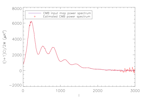
Fig. 1: Estimated CMB power spectrum in the blind approach

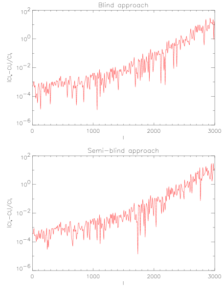
Fig. 2: Relative errors made on the CMB power spectrum estimation in the (quasi) blind approach (top) and in the semi-blind approach (bottom)

The remarkable point is that the estimation errors in both approaches are equivalent. Therefore, it seems that the emission intensity of the components at the different observation frequencies can be estimated in Planck data without loss of accuracy in the linear CMB power spectrum estimation.
In both cases, the method allows to estimate accurately the CMB power spectrum up to $l\simeq 2000$. At smaller scales the dispersion begins to be significant. This result is not surprising since the noise and the beam smoothing effect are important at these scales for all detectors. Also, the estimated power spectrum does not seem to be contaminated by the kinetic SZ.

4.4 Discussion

Semi-blind approach?

As we have seen before, in the case where we estimate the mixing matrix as well as the power spectra of the components, we have fixed to zero the contribution of three components at 857GHz, the only component we assume to be present at this frequency is the galactic dust. This hypothesis, being very realistic, appears to be necessary because we expect that the galactic dust and the galactic synchrotron have quasi proportional power spectra. Without any prior, the method can not separate these two components, but the previous simple procedure of fixing some parameters allows to break the degeneracies and to estimate accurately all the components.

Partial coverage

The galactic components are very inhomogeneous on the sky. In the region of the galactic plane, their intensities are several hundred times stronger than in the outer regions. Since we model the components as homogeneous, the method, when applied on those data, is sub-optimal. However, more accurate CMB power spectrum estimation may be obtained by making a galactic cut, involving a partially covered sky processing. The coefficients obtained from the spherical harmonic decomposition of partially covered sky are correlated. Our spectral matching method can be used on such data and a good choice would be to take bin size $\Delta l$ larger than the correlation length in the power spectrum measurement. The method, in particular, is applicable to data such that from the Archeops balloon-borne experiment in which the sky coverage is about $30\%$ of the whole sky.

5 Conclusion

We have adapted our blind MDMC spectral matching method for the processing of all sky CMB maps. The observations are modeled as a noisy linear mixture of beam-convolved components. By maximizing the likelihood of the system, we estimate the power spectra of the components, their contribution levels at each frequency as well as the noise levels. The method has been applied on full sky Planck simulations containing five components. The spherical harmonics basis was used.
The power spectrum of the CMB is accurately estimated up to $l\simeq 2000$ in bins of size $\Delta l=10$. The comparison between the results obtained in blind and semi-blind approaches shows that the mixing elements can be estimated without loss of accuracy in the CMB power spectrum estimation.

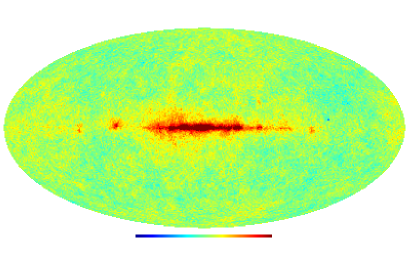
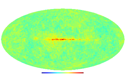
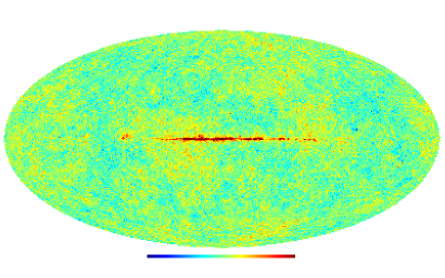
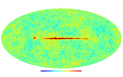
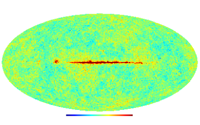
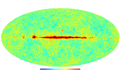
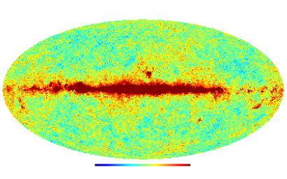
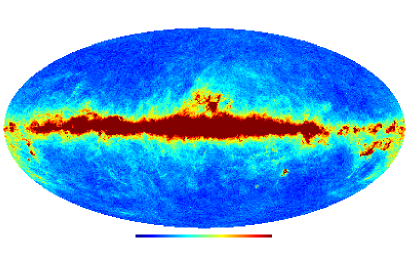
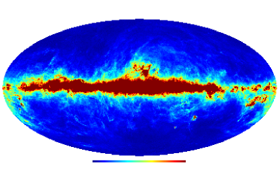
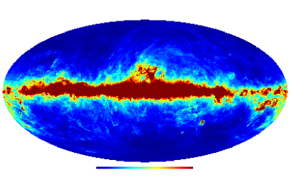
Fig. 3: Simulated Planck observation maps at ten frequencies between 30 and 857 GHz

6 Acknowledgments

We thank the Planck collaboration and in particular V. Stolyarov and R. Kneissl for the full sky simulated maps. Guillaume Patanchon would like to thanks M.A.J. Ashdown for useful discussions while he was visiting Cavendish Laboratory. The HEALPix package [13] (see http://www.eso.org/ science/healpix/) was used for the spherical harmonics decomposition of the input maps.

References

- [1] F. R. Bouchet and R. Gispert, “Foregrounds and cmb experiments. semi-analytical estimates of contamination,” New Astronomy, vol. 4, pp. 443–479, Nov. 1999.
- [2] M. Tegmark and G. Efstathiou, “A method for subtracting foregrounds from multifrequency CMB sky maps,” MNRAS, vol. 281, pp. 1297–1314, Aug. 1996.
- [3] M. P. Hobson, A. W. Jones, A. N. Lasenby, and F. R. Bouchet, “Foreground separation methods for satellite observations of the cosmic microwave background,” MNRAS, vol. 300, pp. 1–29, Oct. 1998.
- [4] V. Stolyarov, M. P. Hobson, M. A. J. Ashdown, and A. N. Lasenby, “All-sky component separation for the planck mission,” MNRAS, vol. 336, pp. 97–111, Oct. 2002.
- [5] S. Prunet, R. Teyssier, S. T. Scully, F. R. Bouchet, and R. Gispert, “Error estimation for the MAP experiment,” Astronomy and Astrophysics, vol. 373, pp. 13–16, July 2001.
- [6] P. Vielva, R. B. Barreiro, M. P. Hobson, E. Martínez-González, A. N. Lasenby, J. L. Sanz, and L. Toffolatti, “Combining maximum-entropy and the Mexican hat wavelet to reconstruct the microwave sky,” MNRAS, vol. 328, pp. 1–16, Nov. 2001.
- [7] C. Baccigalupi, L. Bedini, C. Burigana, G. De Zotti, A. Farusi, D. Maino, M. Maris, F. Perrotta, E. Salerno, L. Toffolatti, and A. Tonazzini, “Neural networks and the separation of cosmic microwave background and astrophysical signals in sky maps,” MNRAS, vol. 318, pp. 769–780, Nov. 2000.
- [8] D. Maino, A. Farusi, C. Baccigalupi, F. Perrotta, A. J. Banday, L. Bedini, C. Burigana, G. De Zotti, K. M. Górski, and E. Salerno, “All-sky astrophysical component separation with Fast Independent Component Analysis (FASTICA),” MNRAS, vol. 334, pp. 53–68, July 2002.
- [9] J. Delabrouille, J. F. Cardoso, and G. Patanchon, “Multi-detector multi-component spectral matching and applications for cmb data analysis,” astro-ph/0211504, submitted to MNRAS.
- [10] J.F. Cardoso, H. Snoussi, J. Delabrouille, and G. Patanchon, “Blind separation of noisy gaussian stationary sources. application to cosmic microwave background imaging,” 2002, in Proc. EUSIPCO Vol. 1, pp 561-564.
- [11] M. Zaldarriaga and U. Seljak, “CMBFAST for Spatially Closed Universes,” The Astrophysical Journal Supplement Series, vol. 129, pp. 431–434, Aug. 2000.
- [12] V. R. Eke, J. F. Navarro, and C. S. Frenk, “The evolution of x-ray clusters in a low-density universe,” ApJ, vol. 503, pp. 569–+, Aug. 1998.
- [13] K.M. Górski, E. Hivon, and B.D. Wandelt, “Analysis issues for large cmb data sets,” 1998, in Proceedinds of the MPA/ESO Cosmology Conference, Evolution of Large-Scale Structure, eds. A.J. Banday, R.S. Sheth and L. Da Costa, Garching.