HST/STIS Spectroscopy of the Intermediate Polar EX Hydrae

Abstract

We present the results of our analysis of six orbits of HST/STIS time-tagged spectroscopy of the intermediate polar, EX Hydrae. The high time and wavelength resolution of the HST/STIS spectra provided an excellent opportunity to study the UV properties of EX Hya. Measurements of the continuum and emission line fluxes corroborate earlier studies that show that the emission line fluxes are modulated more strongly than the continuum flux and originate from the accretion curtains, while the continuum flux originates from the white dwarf photosphere. The measured $K$ amplitude of the narrow emission line radial velocity curve is used to calculate a white dwarf mass of $0.91\pm 0.05{\,M_{\odot}}$. Synthetic white dwarf photosphere and accretion disk spectral models are used to further refine the white dwarf and accretion disk properties. Using the spectral models, it is determined that EX Hya has a white dwarf of mass $0.9{\,M_{\odot}}$, $T=23000$ K, an accretion disk truncated at $2.5{\,R_{\rm WD}}$, and is at a distance of $60$ pc.

1 INTRODUCTION

Intermediate polars (IPs) are a class of magnetic cataclysmic variables in which a white dwarf primary star sustains a magnetic field that is sufficient enough to divert the gravitationally controlled mass transfer. IPs may have a truncated accretion disk (the inner edge being wiped out by the magnetic field) or may be diskless accretors (accreting directly from the ballistic accretion stream), but the defining characteristic that separates IPs from the higher magnetic field polars is an asynchronously rotating white dwarf. As the magnetic field lines of the white dwarf sweep around the inner edge of the accretion disk, curtains of magnetically controlled material form and follow along the field lines until the material impacts the white dwarf surface at or near the magnetic poles, with both upper and lower poles in IPs accreting equally.

EX Hydrae is an IP with a spin period of 67 minutes and an orbital period of 98 minutes, which causes an unusual scenario in which the corotation radius is close to the $L_{1}$ point (King & Wynn, 1999). Magnetically controlled accretion occurs from the inner edge of the disk, and possibly from the outer edge of the disk, as evidenced by dips seen during the bulge dip in EUV light curves of EX Hya (Belle et al., 2002). Radiation from EX Hya is seen to be modulated on both the binary orbital and white dwarf spin periods. Binary modulation is seen in the form of a large bulge dip at phases $\phi_{\scriptscriptstyle 98}=0.5-1.1$ ($\phi_{\scriptscriptstyle 98}$ refers to the binary phase) in the EUV light curve, which is caused by absorption along the line of sight to the emitting poles due to the extended hot spot on the edge of the accretion disk. Continuum emission is modulated sinusoidally over spin phase for all wavelength regimes (e.g., Hellier et al., 1987; Rosen et al., 1991; Belle et al., 2002). Maximum spin phase occurs when the upper accretion pole points away from the observer, allowing a direct view of upper and lower accretion regions; minimum spin flux occurs when the upper pole points towards the observer and the lower pole is self-eclipsed by the white dwarf.

Previous UV observations of EX Hya consist of HUT spectra (Greeley et al., 1997), ORFEUS II and IUE spectra (Mauche, 1999), and HST/FOS spectra (Eisenbart et al., 2002). These observations show that the broad emission lines and the continuum flux are formed in different regions; the emission lines from an optically thick accretion curtain and the continuum from the inner most part of the accretion curtain and the white dwarf itself. Blue-shifted absorption was also seen in the C IV $\lambda 1549$Å emission line. The UV data of EX Hya have also been modeled using a variety of continuum emission sources. The continuum has been fit by a $T=25000$ K blackbody (Greeley et al., 1997), but this same work also showed that a bremsstrahlung model, with $T=74000$ K, or a white dwarf photosphere of $T=26200$ K also fit the data well. Eisenbart et al. (2002) found that a white dwarf photosphere of $T_{\rm eff}=25000\pm 3000$ K (determined from line ratios) fit their FOS spectra well.

2 OBSERVATIONS

Our HST/STIS observations, obtained through DDT time, comprised six orbits and used the E140M grating in Echelle mode. Each orbit produced a time-tagged spectrum consisting of 40 Echelle orders. The E140M grating spans a wavelength range of $1150-1735$Å and has a resolving power of $R=45,800$, which corresponds to a wavelength resolution of $0.013-0.019$Å/pixel throughout the spectrum. The six orbit observation provided complete coverage of EX Hya’s spin orbit, but only $\sim 2/3$ of its binary orbit. Table 1 gives the specific phase coverage of each data set. Each spectrum was processed with IRAF/STSDAS software and the time-tagged data was utilized to bin the spectra into phase resolved components.

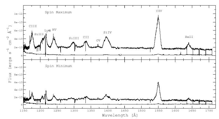
Figure 1: Our HST/STIS data set separated into spin maximum and spin minimum phases. The spectra contain broad emission lines of C III $\lambda 1175$Å, Si III $\lambda 1206$Å, $\lambda 1298$Å, Ly$\alpha$ $\lambda 1216$Å, N V $\lambda 1240$Å, C II $\lambda 1335$Å, O V $\lambda 1371$Å, Si IV $\lambda 1396$Å, C IV $\lambda 1549$Å, and He II $\lambda 1640$Å, along with narrow emission lines N V $\lambda\lambda 1238,1242$Å and O V $\lambda 1371$Å. The thin line in both plots represents the $1\sigma$ errors.

Spectra were extracted for a variety of orbital and spin phase bins. Spin phase bins were determined according to the spin modulation seen in the EUV light curve of EX Hya (Belle et al., 2002) and we have defined spin maximum phases as $\phi_{\scriptscriptstyle 67}=0.865-0.365$ and spin minimum phases as $\phi_{\scriptscriptstyle 67}=0.365-0.865$, where $\phi_{\scriptscriptstyle 67}$ refers to the 67 minute spin ephemeris, $T=2437699.8914(5)+0.046546504(9)\mathrm{E}-7.9(4)\times 10^{-13}\mathrm{E}^{2}$ (Hellier & Sproats, 1992). Spectra extracted throughout the spin period were binned into $\Delta\phi_{\scriptscriptstyle 67}=0.1=402.2$ s phase bins; bins were chosen as such to preserve a moderate signal-to-noise ratio. Three types of binary phased spectra were created: binary phased, spin maximum binary phased, and spin minimum binary phased. For the binary ephemeris, we used $T=2437699.94179+0.068233846(4)\mathrm{E}$ (Hellier & Sproats, 1992). Spin maximum data existed for binary phases $\phi_{\scriptscriptstyle 98}=0.0-0.7$, but spin minimum data only existed for binary phases $\phi_{\scriptscriptstyle 98}=0.0-0.6$. Each binary phase bin has a resolution of $\Delta\phi_{\scriptscriptstyle 98}=0.1=589.5$ s, where $\phi_{\scriptscriptstyle 98}$ refers to the 98 minute orbital period. We used IRAF/SPLOT to analyze the spectra and determine the $1\sigma$ errors we report here. Figure 1 presents our complete spectral data set divided into two phase bins: spin maximum and spin minimum. The spin maximum spectrum has on overall higher continuum level and stronger emission lines than the spin minimum spectrum. Each spectrum exhibits broad emission lines of C III $\lambda 1175$Å, Si III $\lambda 1206$Å, $\lambda 1298$Å, Ly$\alpha$ $\lambda 1216$Å, N V $\lambda 1240$Å, C II $\lambda 1335$Å, O V $\lambda 1371$Å, Si IV $\lambda 1396$Å, C IV $\lambda 1549$Å, and He II $\lambda 1640$Å, along with narrow emission lines N V $\lambda\lambda 1238,1242$Å and O V $\lambda 1371$Å, which appear in all phases except for the early binary phases ($\phi_{\scriptscriptstyle 98}=0.0-0.1$).

3 DISCUSSION AND ANALYSIS

3.1 Continuum

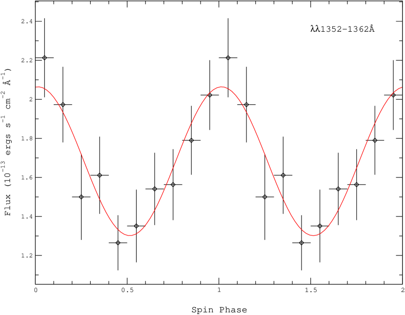
Figure 2: Continuum flux measured at $\lambda\lambda 1352-1362$Å plotted over spin phase and fit with a sinusoidal function of the form $f(10^{-13}{\rm\,ergs\,s^{-1}\,cm^{-2}\,\AA^{-1}})=A+B\sin 2\pi(\phi_{\scriptscriptstyle 67}-\phi_{0})$, where $A=1.683\pm 0.001$, $B=0.381\pm 0.001$, and $\phi_{0}=0.76\pm 0.05$.

Continuum flux measurements were made at three emission line-free wavelength regions along each spectrum: $\lambda\lambda 1352-1362$Å, $\lambda\lambda 1440-1520$Å, and $\lambda\lambda 1565-1620$Å. The results of the $\lambda\lambda 1352-1362$Å measurements are shown in Figure 2 (spin phased). The other two wavelength regions exhibit similar behavior. Error bars on each measurement are RMS values as reported by IRAF/SPLOT. The spin phased continuum flux (Figure 2) is fit well by the sinusoidal function, $f(10^{-13}{\rm\,ergs\,s^{-1}\,cm^{-2}\,\AA^{-1}})=A+B\sin 2\pi(\phi_{\scriptscriptstyle 67}-\phi_{0})$, where $A=1.68$, $B=0.38$, and $\phi_{0}=0.76\pm 0.05$, which places the peak of the light curve at $\phi_{\scriptscriptstyle 67}=0.01\pm 0.05$. The error here is dominated by the fact that each phase bin measurement was confined within the $\Delta\phi_{\scriptscriptstyle 67}=0.1$ phase bin resolution of the data. The continuum flux is modulated by $B/A=23\%$. The peak in UV continuum flux is earlier than that of the EUV emission, which occurs at $\phi_{\scriptscriptstyle 67}=0.115\pm 0.001$ (Belle et al., 2002). As both the HST and EUVE observations of EX Hya occurred simultaneously, an error in the ephemeris is ruled out as a cause for phase difference in peak continuum fluxes; rather, the phase disparity is likely a result of distinct EUV and UV continuum emission sites. The sinusoidal fits to all of the spin phased UV continuum wavelength regions are given in Table 2.

The spectra were also measured over binary phase, and, in agreement with previous studies (e.g., Hellier et al., 1987), we found that the continuum flux did not exhibit coherent modulation over the binary orbital period.

3.2 Emission Lines

3.2.1 Broad Emission Lines

The broad emission lines were fit with single Gaussian functions and a linear continuum, using IRAF/SPLOT, to determine parameters such as central wavelength, flux, FWHM, and equivalent width. The Ly$\alpha$ and Si III $\lambda 1206$Å lines were not measured because they are blended during the spin maximum phases.

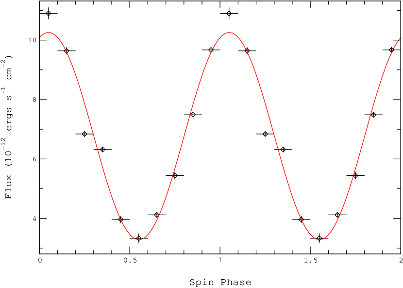
Figure 3: C IV broad emission line flux plotted over spin phase and fit with a sinusoidal function (solution given in Table 3).

Over spin phase, the emission line fluxes exhibit a sinusoidal shape (C IV is shown as an example in Figure 3), and can be fit well with a sinusoidal function of the form $f(10^{-12}{\rm\,ergs\,s^{-1}\,cm^{-2}})=A+B\sin 2\pi(\phi_{\scriptscriptstyle 67}-\phi_{0})$. The solutions for each line are given in Table 3. The emission peaks near $\phi_{\scriptscriptstyle 67}\sim 0.05-0.1$ for each line. Considering the error of $0.05\phi_{\scriptscriptstyle 67}$ on each phase bin, the emission line fluxes peak at roughly the same phase as the continuum flux ($\phi_{\scriptscriptstyle 67}\sim 0$). C III $\lambda 1175$Å has the greatest modulation, at $73\%$, but all of the lines are strongly modulated by around $50\%$. Compare this with the continuum with a flux modulation of only $\sim 20-25\%$. While both the continuum and emission lines are modulated sinusoidally over spin phase, the difference in the modulation amplitude suggests that the continuum and emission lines have different formation sites. Over binary phase the emission line flux is not modulated coherently. Comparison of the emission line fluxes over binary and spin phase demonstrates that the flux modulations are clearly a function of spin phase, rather than binary phase.

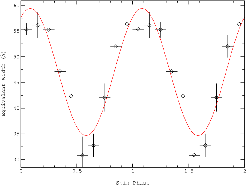
Figure 4: Equivalent width of the C IV broad emission line phased over the spin period. Solutions for the sinusoidal fits to all of the broad emission lines are given in Table 4.

Equivalent widths (EWs) of strong UV emission lines from optically thin plasmas are typically on order of 100s of Ångstroms. The EWs of the emission lines appearing in the EX Hya spectra are smaller than expected for optically thin plasma emission. C IV, which has the largest EW of all the broad emission lines, is shown as an example in Figure 4 (solutions for the sinusoidal fits to all of the lines are given in Table 4). There are two possible scenarios that may explain the observed EWs. The first is that optically thick material is responsible for the emission lines. The second is that the optically thin material is only weakly emitting and another form of radiation, such as cyclotron emission, may play an important role in the radiative cooling of the accretion curtains. If the latter is true, evidence should be seen in the form of cyclotron humps; for a magnetic field strength of $B\sim 5$ MG, the first cyclotron harmonic should appear around 10$\mu$. The almost triangular shapes of the lines implies that they are not from a purely optically thin material, thus it is likely that both optically thin and optically thick emission contributes to each emission line.

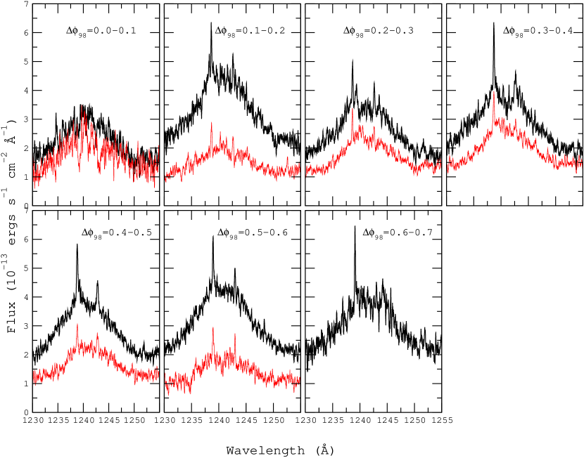
Figure 5: N V $\lambda 1240$Å emission line profile evolution over the binary orbit and separated into spin maximum (thick line) and spin minimum (thin line). For all phases except $\phi_{\scriptscriptstyle 98}=0.0-0.1$, the line profile extracted at spin maximum is greater in flux than the spin minimum line. Also note the narrow emission lines that appear during phases $\phi_{\scriptscriptstyle 98}=0.1-0.7$ and that exhibit a double-peaked nature in the spin maximum spectrum near binary phases $\phi_{\scriptscriptstyle 98}=0.1-0.2$, while the blue component only is visible in the spin minimum line profile.

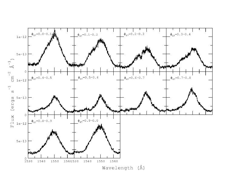
Figure 6: C IV $\lambda 1549$Å line over spin phase. Note the blue-shifted absorption that appears during phases $\phi_{\scriptscriptstyle 67}=0.2-0.3$ and the asymmetric profile as the line evolves over spin phase.

Figures 5 and 6 present two examples of the broad emission line evolution over binary and spin orbit. The N V $\lambda 1240$Å line shown in Figure 5 has been separated into spin maximum (thick line) and spin minimum (thin line) and phased over the binary orbit. The line retains roughly the same form throughout the binary orbit for both spin phases. Aside from binary phase bin $\Delta\phi_{\scriptscriptstyle 98}=0.0-0.1$, the flux of the spin maximum line is constantly greater than the flux of the spin minimum line. This suggests that the lines are formed in a region that would be partially absorbed or occulted during spin minimum phases, i.e. the inner part of the accretion curtain. Also of interest is the lack of narrow emission lines during binary phases $\Delta\phi_{\scriptscriptstyle 98}=0.0-0.1$, which correspond to the egress of the bulge dip; absorption features appear in their place. The narrow lines will be discussed in further detail in §3.2.2. The fact that the lines have roughly the same amount of absorption during $\Delta\phi_{\scriptscriptstyle 98}=0.0-0.1$ implies that the lines are formed interior to the bulge.

If the change in flux of the broad emission lines between spin phases maximum and minimum is due to absorption through the accretion curtain, we can estimate the density of the curtains from the amount of absorption. Using the simple relation of $I=I_{0}e^{-\tau}$, we may first deduce $\tau$ and then assume a Kramer’s opacity law to determine the density. The physical size of the accretion curtains must first be estimated. At most, the radial extent of the footprint of the curtain on the disk could be the entire truncated accretion disk and at the least, it would only be a small fraction of the disk size. The disk size was determined by measuring optical emission lines (using the optical data obtained by us during this campaign) to determine the inner and outer accretion disk radius, assuming a Keplerian accretion disk. We considered two white dwarf masses (see §3.3), ${\,M_{WD}}=0.90{\,M_{\odot}}$ and ${\,M_{WD}}=1.33{\,M_{\odot}}$, and calculated the disk radii corresponding to each white dwarf mass ($R_{\rm inner}=1.6-2.3\times 10^{9}{\rm\,cm}$ and $R_{\rm outer}=2.5-5.9\times 10^{9}{\rm\,cm}$). Several different physical sizes, $S$, of the accretion curtain were used for our density calculation. We take $S=aR_{\rm disk}$, where $a=0.01,0.10,0.50$ and $1.0$. In this way we were able to sample a range of physical depths for the accretion curtain. The emission line fluxes were measured during spin maximum and spin minimum, excluding binary phases of the bulge dip. This ensures that material associated with the bulge, which is also responsible for absorption at certain spin phases, will not be mistakenly identified with accretion curtain material. Five emission lines were used for this calculation; C III, N V, Si IV, C IV, and He II. Si III $\lambda 1296$Å and C II were not used due to their ambiguous line profiles during spin minimum. For each white dwarf mass and corresponding $S$ values, we find that $\tau=0.7-1.1$ and the density ranges between $10^{-10}-10^{-9}\,{\rm g\,cm^{-3}}$ for all values of $S$. If we assume that the absorbing material is pure hydrogen, we obtain a number density of $N_{\rm H}=7\times 10^{13}-8\times 10^{14}{\rm\,cm}^{-3}$ within the accretion curtains.

The C IV $\lambda 1549$Å emission line has a blue-shifted absorption component that appears during spin phases $\Delta\phi_{\scriptscriptstyle 67}\sim 0.2-0.8$ as evidenced in Figure 6. A similar feature was also observed in the C IV line in HUT data during spin phases $\Delta\phi_{\scriptscriptstyle 67}=0.36-0.48$ (their data only extended through $\phi_{\scriptscriptstyle 67}=0.5$, Greeley et al. 1997). Although their C IV line is phased into finer orbital bins, our C IV line clearly shows an absorption component that begins prior to $\phi_{\scriptscriptstyle 67}=0.3$ and evolves into an absorption that eats away the blue wing of the emission line. At phases $\phi_{\scriptscriptstyle 67}=0.2-0.3$, the blue absorption has a FWHM of $\sim 275{\rm\,km\,s^{-1}}$ and is blue-shifted by $\sim 615{\rm\,km\,s^{-1}}$ from the center of the C IV doublet. This is slightly less than the value of $\sim 1000{\rm\,km\,s^{-1}}$ reported by Greeley et al. (1997) for their blue C IV absorption feature.

C III, N V, and C II also show a blue absorption component during spin phases $\phi_{\scriptscriptstyle 67}\sim 0.2-0.7$. The N V absorption component has a FWHM of $\sim 400{\rm\,km\,s^{-1}}$ and is blue-shifted by $\sim 700{\rm\,km\,s^{-1}}$ from the center of the line. The C III absorption component is really too shallow to accurately measure, though it is visible during spin phases $\phi_{\scriptscriptstyle 67}\sim 0.2-0.7$. The C II line seems to have a blue-shifted absorption component throughout the entire spin phase. Its FWHM ranges from $655{\rm\,km\,s^{-1}}$ at $\phi_{\scriptscriptstyle 67}=0.4-0.5$ to $\sim 200{\rm\,km\,s^{-1}}$ at $\phi_{\scriptscriptstyle 67}=0.0-0.1$ while the blue-shift from the center of the emission line remains fairly constant at $\sim 1400{\rm\,km\,s^{-1}}$. However, the C II absorption feature is associated with a white dwarf absorption line (see §3.4), which may influence the motion of the line.

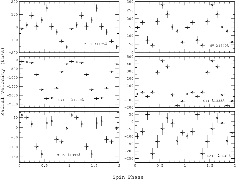
Figure 7: Broad emission line radial velocities phased on the spin period. Si III is the only line that appears to have a sinusoidal shape; the other radial velocity curves are somewhat double-peaked, with one peak occurring near $\phi_{\scriptscriptstyle 67}=0.2$ and the second occurring at $\phi_{\scriptscriptstyle 67}=0.5$.

Radial velocity curves for the broad emission lines are shown in Figure 7 phased over the spin period. The spin phased radial velocity curves present surprising results. In previous EX Hya observations (e.g., Hellier et al., 1987), the maximum blue-shift of the optical emission lines observed around $\phi_{\scriptscriptstyle 67}=0.0$ has been used to place the origin of these lines in the accretion curtain; while the upper pole points away from us, material flowing into the pole will be at its maximum blue-shift. We see that three lines exhibit this behavior: C III, N V, and C II. Si III, Si IV, and He II, on the other hand, have maximum blue-shifts closer to $\phi_{\scriptscriptstyle 67}\sim 0.5$. A double peaked structure is visible in all but the Si III radial velocity curve.

3.2.2 Narrow Emission Lines

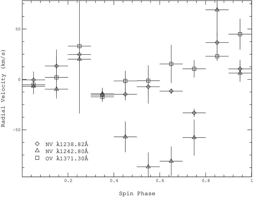
Figure 8: Narrow emission line radial velocities phased on the spin orbit. The radial velocity curve of each line is double-peaked, with maxima occurring at $\phi_{\scriptscriptstyle 67}=0.2$ and $\phi_{\scriptscriptstyle 67}=0.8$; the N V $\lambda 1242$Å component shows the strongest modulation.

Three narrow emission lines appear in the HST spectra: N V $\lambda\lambda 1238.8,1242.8$Å and O V $\lambda 1371.3$Å, and represent the two highest ionization energy lines present in the spectrum, with $\chi_{\rm NeV}=98$ eV and $\chi_{\rm OV}=114$ eV. These lines have FWHM$\sim 0.2$Å and are visible over both spin and binary orbit, and only disappear during binary phases $\phi_{\scriptscriptstyle 98}=0.0-0.1$, which correspond to the egress of the bulge dip. A radial velocity curve over spin phase is shown for the narrow emission lines in Figure 8. Each radial velocity curve has a double-peaked structure, although the O V and N V $\lambda 1238$Å lines are less modulated than the N V $\lambda 1242$Å line. For each line the velocities tend to be blue for two reasons: one, only two-thirds of the binary orbit, $\phi_{\scriptscriptstyle 98}=0.0-0.7$, are (unevenly) sampled in each spin phase bin and two, a $\gamma-$velocity has not been subtracted. Previous measurements of the $\gamma-$velocity (derived from optical spectroscopy) range from $-9\pm 35{\rm\,km\,s^{-1}}$ (Gilliland, 1982) to $-180{\rm\,km\,s^{-1}}$ (Hellier et al., 1987), and we will show below that we obtain a value slightly different from the Gilliland (1982) and Hellier et al. (1987) results.

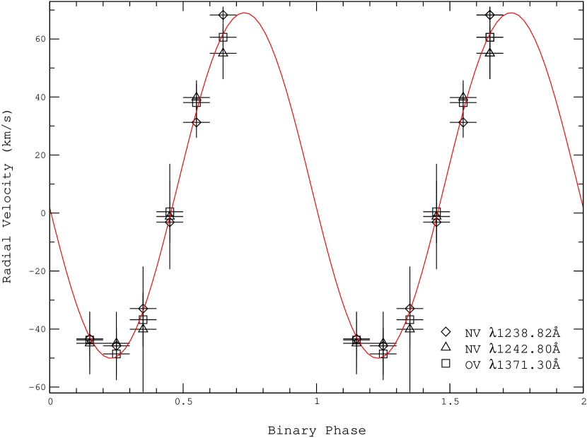
Figure 9: Binary phased radial velocity curve for the narrow emission lines. This radial velocity curve is fit nicely with a sinusoidal function of the form $v=\gamma+K\sin 2\pi(\phi_{\scriptscriptstyle 98}-\phi_{0})$, with $\gamma=9.5\pm 3{\rm\,km\,s^{-1}}$, $K=59.6\pm 2.6{\rm\,km\,s^{-1}}$ and $\phi_{0}=0.98\pm 0.05$.

The radial velocities of the narrow emission lines over the binary phase are shown in Figure 9 and can be fit with a sinusoidal function of the form $v=\gamma+K\sin 2\pi(\phi_{\scriptscriptstyle 98}-\phi_{0})$, with $\gamma=9.5\pm 3{\rm\,km\,s^{-1}}$, $K=59.6\pm 2.6{\rm\,km\,s^{-1}}$ and $\phi_{0}=0.98\pm 0.05$. The $K$ amplitude derived here is comparable with a previously determined value of $K_{1}=69\pm 9{\rm\,km\,s^{-1}}$ (Hellier et al., 1987). The small velocities, the clear sinusoidal modulation of the velocities, and the $K$ amplitude suggest that these lines are formed near or on the white dwarf surface. A high temperature emission region for these lines increases the likelihood that the lines are not contaminated by emission from the accretion disk. This narrow line radial velocity curve is therefore likely to be a true representation of the motion of the white dwarf, as compared to optical (disk) emission lines that have been used previously to determine the $K_{1}$ amplitude and the $\gamma-$velocity (e.g., Hellier et al., 1987). We would like to note that the proximity of the narrow line emission region to the white dwarf surface should cause these lines to be gravitationally redshifted. Unfortunately, without an accurate $\gamma$-velocity measurement, it is impossible to separate the gravitationally redshift from the $\gamma$-velocity of the narrow emission line radial velocity curve.

The narrow emission lines appear to be double-peaked during certain spin phases. The N V doublet shows a strong double-peaked profile during spin phases $\phi_{\scriptscriptstyle 67}=0.1-0.3$, $\phi_{\scriptscriptstyle 67}=0.5-0.6$, and $\phi_{\scriptscriptstyle 67}=0.9-1.0$. O V is double-peaked during spin phases $\phi_{\scriptscriptstyle 67}=0.0-0.3$, $\phi_{\scriptscriptstyle 67}=0.4-0.6$ and $\phi_{\scriptscriptstyle 67}=0.7-0.8$. These phases roughly correspond to spin maximum phases. Close inspection of Figure 5 also shows the double-peaked nature of the N V line during spin maximum and that during spin minimum, it is only the blue component of the double-peaked line that is still visible. The radial velocities of these lines over binary phase tell us that they originate close to the white dwarf surface. The double-peaked nature of the lines suggest a two velocity component as their origin. We propose that these lines are formed in a wind or material outflowing from the poles. During spin maximum, we have a direct view of both poles (possibly not a direct view of the northern pole as it points away from us, but a wind would clearly be seen) giving us both red and blue-shifted components. At spin minimum, when the upper pole points towards the observer, the lower pole and its (red-shifted) emission is blocked from view; only the blue-shifted narrow line component would be seen at these phases. As discussed in §3.2.1, evidence of a wind is also seen in the form of blue-shifted absorption in several of the broad emission lines.

3.3 Mass Determinations

In order to calculate a white dwarf mass, a value for the secondary mass must be estimated. Previous studies have used an $M_{2}$ value determined from a zero age main sequence (ZAMS) mass-radius relation applied to the Roche lobe radius for a given binary orbital period. Hellier et al. (1987) found $M_{2}=0.128{\,M_{\odot}}$ using the ZAMS mass-radius relation given in Patterson (1984) and an earlier study used the relation presented in Warner (1976) to find $M_{2}=0.18{\,M_{\odot}}$. We use a value based on an up-to-date mass-radius relation (Howell et al., 2001) expressed in the form of

$$M_{2}=0.08f^{-1.95}P_{\rm orb}^{1.3}$$ (1)

where $P_{\rm orb}$ is the binary orbital period in hours and $f$ is a factor that describes the bloating of the secondary star in systems above the period gap. For the EX Hya orbital period of 1.6 hr and $f=1$, we calculate $M_{2}=0.152{\,M_{\odot}}$, a value slightly higher than the $0.128{\,M_{\odot}}$ that has been used previously to determine the white dwarf mass.

Using the $K_{1}$ amplitude determined from our UV narrow emission line radial velocity curve, we expect to obtain an unambiguous determination of the mass of the white dwarf if our value of $M_{2}$ is correct. We employ a modified form of Kepler’s third law,

$$\sin^{3}i=\frac{K_{1}^{3}P_{\rm orb}}{2\pi GM_{2}}\left(\frac{q+1}{q}\right)^{2}$$ (2)

and solve for $q$ in order to determine ${\,M_{WD}}$. For $i=78\pm 1^{\circ}$ (Hellier et al., 1987), $M_{2}=0.152{\,M_{\odot}}$, and $K_{1}=59.6\pm 2.6{\rm\,km\,s^{-1}}$, we determine a white dwarf mass, ${\,M_{WD}}=1.33\pm 0.11{\,M_{\odot}}$. This value is considerably higher than $0.78\pm 0.17{\,M_{\odot}}$, which was determined by Hellier et al. (1987), and the even lower values of $\sim 0.5{\,M_{\odot}}$ that have been determined from X-ray studies (e.g., Fujimoto & Ishida 1997). Although our $K_{1}$ amplitude agrees within the errors with the value measured by Hellier et al. (1987), our white dwarf mass does not agree with theirs due to the larger secondary mass used in the above calculation.

Smith, Cameron, & Tucknott (1993) applied the method of skew-mapping to detect the secondary stars in cataclysmic variables. Applying this to EX Hya, they found a velocity amplitude for the secondary motion of $K_{2}=356\pm 4{\rm\,km\,s^{-1}}$. This amplitude, along with our measured value of $K_{1}$ and calculated value of $M_{2}$ may be used to apply another determination of $M_{1}$ using $K_{1}/K_{2}=M_{2}/M_{1}$. This method gives a white dwarf mass of ${\,M_{WD}}=0.91\pm 0.05{\,M_{\odot}}$, which is $\sim 30\%$ lower than the value determined above, although still larger than the earlier estimates (e.g., Hellier et al. 1987).

3.4 Spectral Modeling

Discerning exactly which components of the binary system are contributing UV continuum flux (and at which spin phases) is an important issue for thorough modeling of the HST spectra of EX Hya. Spin maximum phase would seem to be the most likely time in which we would have a direct view of the white dwarf, but are there other components also visible during this phase? The accretion poles (shock regions) are strong emitters in the X-ray and EUV (Belle et al., 2002). The irradiated material in the accretion curtain close to the pole, however, may emit reprocessed X-ray and EUV radiation as UV radiation, thus adding another UV emission component to the system. The accretion disk, although truncated, is likely to add to the UV continuum emission as well.

To model our HST spectra with a white dwarf photosphere, we must determine which spectrum is the best representation of the white dwarf by ascertaining which of the different components discussed above contribute to the spin maximum and spin minimum spectra. Visual inspection of the spin maximum and minimum spectra reveals their differences; the red-ward slopes of each spectrum are roughly the same while the blue end of the spin minimum spectrum has a lower flux than that of the spin maximum spectrum. There are two possible cases to consider; $1-$ spin minimum is the true white dwarf spectrum and the accretion curtain is optically thin to the white dwarf continuum. Spin maximum therefore contains an additional continuum component that could be the accretion region located at either pole. $2-$ The spin minimum spectrum is absorbed by the accretion curtains and the spin maximum spectrum is the true white dwarf spectrum plus an additional continuum component. These two options outline the occultation (1) versus absorption (2) models. For option 1, spin phased modulation is due to occultation of an emitting pole, while option 2 dictates that spin phased modulation is due to UV flux being absorbed by the accretion curtains.

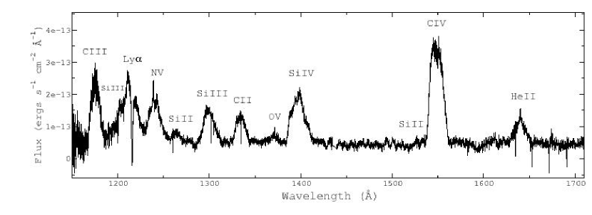
Figure 10: Spin maximum - spin minimum difference spectrum.

For either model option, the spin maximum spectrum has added UV continuum components. This is evidenced by the fact that the blue slopes of the spin maximum and minimum spectra are not equal. If the spin modulation were simply due to absorption, the spin minimum spectrum would retain the same slope as that of the spin maximum spectrum. (This assumes a gray absorber, which is valid over the small, $\sim 600$Å, wavelength range covered by the HST spectra.) We show the difference spectrum of EX Hya, which is the spin maximum minus the spin minimum spectrum, in Figure 10. This spectrum represents the additional UV continuum and emission line components that are seen during spin maximum phases. Considering the above arguments, we rule out the spin maximum spectrum as representative of only the UV white dwarf continuum flux. For option 1 to be viable, the accretion curtains near the poles would have to be dense enough to absorb the flux emitted from the accretion region. While the outer curtains are optically thin, it is likely that the curtain close to the pole is optically thick and will absorb emitted radiation from the accretion pole. We therefore suggest the case that the spin minimum spectrum is the better representation of the pure white dwarf spectrum and that a blue blackbody and emission line component (or multiple components) is seen in addition to the white dwarf during spin maximum. Flux contributed by the truncated accretion disk must also be considered at all spin phases.

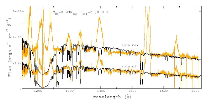
Figure 11: An ${\,M_{WD}}=0.90{\,M_{\odot}}$, $T_{\rm eff}=23000$ K white dwarf photosphere model (black spectra) fit to the spin maximum (top) and spin minimum (bottom) spectra (gray spectra). The slope and absorption lines of the spin minimum spectrum are fit better by the white dwarf photosphere model than the spin maximum spectrum.

We first created white dwarf photosphere models using TLUSTY and SYNSPEC (Hubeny, 1988) for the two white dwarf masses computed in §3.3, $0.90{\,M_{\odot}}$ ($\log\,g=8.5$) and $1.33{\,M_{\odot}}$ ($\log\,g=9.4$). We modeled white dwarf photospheres of solar composition and considered temperatures ranging from $T_{\rm eff}=19000\,{\rm K}\,-35000$ K (in steps of $1000$ K). Although it was decided that the spin minimum spectrum would be the best representation of the white dwarf spectrum, the model photospheres were fit to the spin maximum and minimum spectra in order to insure that the spin minimum spectrum was indeed the best choice. For each fit, the broad emission lines in the HST spectrum were masked, except for the wavelength range including the Si III$\lambda 1298$Å and C II$\lambda 1335$Å emission lines because of the white dwarf absorption components that appear between these emission features. Our best fitting $0.90{\,M_{\odot}}$, $T_{\rm eff}=23000$ K white dwarf photosphere model is shown in Figure 11 fit to both the spin maximum and spin minimum spectra. The spin minimum fit has a reduced $\chi^{2}$ of 1.7, and scaled to the HST continuum fluxes, gives a distance to EX Hya of 54 pc. The spin maximum fit has a reduced $\chi^{2}$ value of 3.3 and scaled to the HST continuum fluxes gives a distance of 46 pc.

Note that many of the absorption features appearing between the Si III and C II in the spin minimum spectrum are fit well by the white dwarf photosphere model. The slope of the model spectrum also produces a better match to that of the spin minimum spectrum than the maximum spectrum. These facts, coupled with the lower reduced $\chi^{2}$ value of the spin minimum fit, corroborate with our earlier statement that the spin minimum phases are the ideal phases during which to model the white dwarf photosphere. We therefore use only the spin minimum spectrum in our following model fits.

White dwarf photospheres with temperatures of $T_{\rm eff}=23000-35000$ K (in steps of $2000$ K) were created for ${\,M_{WD}}=1.33{\,M_{\odot}}$. The best fit model to the spin minimum spectrum has a temperature of $T_{\rm eff}=25000$ K, but while this model provides a good fit, it also places the distance of EX Hya at $30$ pc! This distance varies greatly from the distances of $65-100$ pc that have been determined in previous studies (e.g., Hellier et al., 1987; Eisenbart et al., 2002). We explored the relationship of distance versus white dwarf photosphere temperature for both white dwarf masses over a range of temperatures and found that, for ${\,M_{WD}}=1.33{\,M_{\odot}}$, a white dwarf temperature of $T_{\rm eff}=35000$ K would be required to achieve a distance of 55 pc (when scaled to the spin minimum spectrum). An ${\,M_{WD}}=1.33{\,M_{\odot}}$, $T_{\rm eff}=35000$ K white dwarf photosphere model was considered for the spin minimum spectrum, but the slope did not match the HST continuum slope. However, before we completely rule out either white dwarf mass, we must also consider the accretion disk contribution to the UV continuum flux.

Accretion disk models were created using TLUSDISK, SYNSPEC, and DISKSYN (Hubeny, 1988; Wade & Hubeny, 1998) for white dwarf masses of ${\,M_{WD}}=0.90{\,M_{\odot}}$ and ${\,M_{WD}}=1.33{\,M_{\odot}}$. We used an accretion rate of $10^{16}{\rm g\,s}^{-1}$ (Fujimoto & Ishida, 1997) and an inclination of $i=78^{\circ}$ (Hellier et al., 1987). In order to determine the radius at which the disk should be truncated, the inner disk radius was determined from our optical spectra. For a Keplerian disk, the highest velocities in an emission line originate from the inner disk. The optical line wings, therefore, should map to the inner edge of the disk. The H$\alpha$ $\lambda 6563$Å line profile in each of our optical spectra was used to determine the velocities at the blue and red wings. For a ${\,M_{WD}}=0.90{\,M_{\odot}}$ white dwarf, these velocities map to an inner accretion disk radius of $R_{\rm inner}=2.5{\,R_{\rm WD}}$ ($1.6\times 10^{9}{\rm\,cm}$) and for a ${\,M_{WD}}=1.33{\,M_{\odot}}$ white dwarf, the inner radius becomes $R_{\rm inner}=9.0{\,R_{\rm WD}}$ ($2.3\times 10^{9}{\rm\,cm}$). Previous modeling studies (e.g., Greeley et al., 1997) have assumed $R_{\rm inner}\sim 5{\,R_{\rm WD}}$ ($3.5\times 10^{9}{\rm\,cm}$) and optical spectroscopy by Hellier et al. (1987) gave $R_{\rm inner}=6\times 10^{9}{\rm\,cm}$ for ${\,M_{WD}}\sim 0.8{\,M_{\odot}}$.

Two different accretion disk models must be created for the two different white dwarf masses we have been using. ${\,M_{WD}}=0.90{\,M_{\odot}}$ and $\dot{M}=10^{16}\,{\rm g\,s}^{-1}$ correspond to Models $n$ and $p$ of Wade & Hubeny (1998) and ${\,M_{WD}}=1.33{\,M_{\odot}}$ with the same accretion rate matches most closely with Models $y$ and $z$. Model $n$ ($p$) has UV flux contributing annuli that extend to $6.2{\,R_{\rm WD}}$ ($9.40{\,R_{\rm WD}}$), and Model $y$ ($z$) has contributing annuli that extend out to $14.3{\,R_{\rm WD}}$ ($21.7{\,R_{\rm WD}}$); the last annulus in each model has $T\sim 10000$ K. Although it would seem that the synthetic spectra for each disk model would be different because of the different truncation points, the truncated accretion disk spectra are in fact quite similar. This is due to the fact that the more massive white dwarf has a hotter accretion disk and while the disk is truncated at a greater radius than the less massive white dwarf, an approximately equal amount of UV flux is still emitted from the remaining annuli.

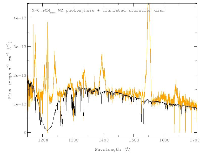
Figure 12: Best fit white dwarf photosphere plus truncated accretion disk model for EX Hya. This model uses ${\,M_{WD}}=0.90{\,M_{\odot}}$, $T=23000$ K, and $R_{\rm inner}=2.5{\,R_{\rm WD}}$, and is fit to the spin minimum spectrum. Scaled to the EX Hya spectra, this model gives a distance of 60 pc.

The truncated disk models were added to the white dwarf photosphere models using the following method: the photosphere model and disk model were scaled separately to a distance, $d$, and then summed together. The summed spectrum was then fit to the observed spectrum. The distance, $d$, was modified until the summed spectrum produced a good fit to the observed spectrum. The summed model fits were judged by visual inspection, rather than by a formal fitting routine. For ${\,M_{WD}}=0.90{\,M_{\odot}}$, we found that a $T_{\rm eff}=23000$ K white dwarf plus the truncated disk produced the best fit at a distance $d=60$ pc. The ${\,M_{WD}}=1.33{\,M_{\odot}}$ model showed a best fit for $T_{\rm eff}=25000$ K plus the truncated disk at a distance of $d=33$ pc. The ${\,M_{WD}}=0.90{\,M_{\odot}}$ fit is shown in Figure 12, as we definitively rule out the higher mass model below.

The white dwarf photosphere plus truncated accretion disk model fits to the HST fluxes give two different distances: the $0.90{\,M_{\odot}}$ white dwarf model gives $d=60$ pc, while the $1.33{\,M_{\odot}}$ white dwarf gives $d=33$ pc. We can check these distances independently by using Bailey’s method (Bailey, 1982), which uses the $K-$band magnitude and measured surface brightness values for K-M single stars to determine a distance;

$$\log\,d=\frac{K}{5}+1-\frac{S_{K}}{5}+\log\left(\frac{R_{2}}{R_{\odot}}\right)$$ (3)

where $S_{K}$ is the surface brightness. Using $K=11.705(28)$ from the 2MASS survey (Hoard et al., 2002), $S_{K}=4.5\pm 0.5$ for an M3 main sequence star (Dhillon et al., 1997), $R_{2}=0.17R_{\odot}$, and the secondary $K-$band flux contribution as $75\pm 25\%$ (Dhillon et al., 1997), we determine the distance to EX Hya to be $d=54^{+12}_{-7}$ pc. This effectively rules out the $1.33{\,M_{\odot}}$, $T_{\rm eff}=25000$ K white dwarf, as the distance determined by this model is 33 pc.

The greatest uncertainties in the distance calculation and the white dwarf mass determination are the secondary star mass and spectral type. An M3 main sequence secondary star (determined from IR spectra, Dhillon et al., 1997) has a mass of $\sim 0.3{\,M_{\odot}}$. This is not consistent with the mass determined using the ZAMS mass-period relation (Equation 1), which gave the secondary mass as $0.15{\,M_{\odot}}$. Returning to Equation 2, we find that a secondary mass of $0.12{\,M_{\odot}}$ would be required to obtain ${\,M_{WD}}=0.9{\,M_{\odot}}$. A more accurate secondary mass will be needed to aid future distance and white dwarf mass determinations of EX Hya.

4 CONCLUSION

We have made an accurate measurement of the $K$ amplitude of the white dwarf based on the narrow emission line radial velocity curve. The small velocities and high ionization temperatures required for production of the N V and O V emission lines indicate that they are formed close to the white dwarf, and therefore, the $K_{1}=59.6\pm 2.6{\rm\,km\,s^{-1}}$ value that we have measured is an accurate representation of the motion of the white dwarf within the binary system.

Synthetic spectral models for a white dwarf photosphere and truncated accretion disk were made using TLUSTY and SYNSPEC (Hubeny, 1988). Based on spectral fits using a white dwarf photosphere model, we determined that the spin minimum phases are the best representation of the white dwarf spectrum, i.e., occultation of (one of) the emitting poles is responsible for the continuum modulation seen over the white dwarf spin phase. The distance we derive based on spectral modeling, $d\approx 60$ pc, agrees well with two recent measurements; Eisenbart et al. (2002) determine $d=65\pm 11$ pc using Bailey’s method and a $K$ magnitude derived from their infrared spectra, while a recent parallax measurement has placed the distance to EX Hya at $\sim 60$ pc (K. Beuermann, private communication). This implies that our spectral modeling parameters for a solar composition white dwarf photosphere and truncated accretion disk - ${\,M_{WD}}=0.9{\,M_{\odot}}$, $T=23000$ K, and $R_{\rm inner}=2.5{\,R_{\rm WD}}$ - represent EX Hya well.

Table 1: HST spectra phase coverage.

HST Data set	HJD start-stop	Spin Phase	Binary Phase
o68301010	$2451682.894-2451682.919$	$0.67-0.22$	$0.32-0.69$
o68301020	$2451682.950-2451682.982$	$0.88-0.55$	$0.14-0.60$
o68301030	$2451683.017-2451683.049$	$0.32-0.99$	$0.13-0.59$
o68302010	$2451694.622-2451694.647$	$0.62-0.17$	$0.19-0.56$
o68302020	$2451694.680-2451694.712$	$0.87-0.55$	$0.04-0.50$
o68302030	$2451694.747-2451694.779$	$0.32-0.99$	$0.03-0.48$

Table 2: Sinusoidal fits to the continuum fluxes.

Continuum Region	$A$	$B$	$\phi_{0}$	$B/A$
$\lambda\lambda 1352-1362$Å	$1.683\pm 0.001$	$0.381\pm 0.001$	$0.77\pm 0.05$	$23\%$
$\lambda\lambda 1440-1520$Å	$1.554\pm 0.001$	$0.315\pm 0.001$	$0.76\pm 0.05$	$20\%$
$\lambda\lambda 1565-1620$Å	$1.375\pm 0.001$	$0.337\pm 0.001$	$0.78\pm 0.05$	$24\%$

Table 3: Sinusoidal fits to the broad emission line fluxes.

Ion	$A$	$B$	$\phi_{0}$	$B/A$
C III	$1.897\pm 0.004$	$1.381\pm 0.003$	$0.81\pm 0.05$	$73\%$
N V	$1.694\pm 0.002$	$0.864\pm 0.001$	$0.80\pm 0.05$	$51\%$
Si III	$1.183\pm 0.001$	$0.618\pm 0.001$	$0.83\pm 0.05$	$52\%$
C II	$1.288\pm 0.001$	$0.555\pm 0.001$	$0.81\pm 0.05$	$43\%$
Si IV	$2.895\pm 0.002$	$1.732\pm 0.001$	$0.81\pm 0.05$	$60\%$
C IV	$6.771\pm 0.004$	$3.490\pm 0.002$	$0.80\pm 0.05$	$52\%$
He II	$0.963\pm 0.001$	$0.554\pm 0.001$	$0.82\pm 0.05$	$58\%$

Table 4: Sinusoidal fits to the broad emission line equivalent widths.

Ion	$A$	$B$	$\phi_{0}$	$B/A$
C III	$10.84\pm 0.02$	$-5.35\pm 0.01$	$0.81\pm 0.05$	$49\%$
N V	$10.44\pm 0.01$	$-1.738\pm 0.001$	$0.82\pm 0.05$	$17\%$
Si III	$7.20\pm 0.01$	$-2.141\pm 0.002$	$0.90\pm 0.05$	$30\%$
Si IV	$17.06\pm 0.01$	$-6.638\pm 0.003$	$0.82\pm 0.05$	$39\%$
C IV	$47.03\pm 0.03$	$-12.37\pm 0.01$	$0.83\pm 0.05$	$26\%$
He II	$7.39\pm 0.01$	$-2.078\pm 0.002$	$0.85\pm 0.05$	$28\%$

References

- Bailey (1982) Bailey, J. 1982, MNRAS, 197, 31
- Belle et al. (2002) Belle, K. E., Howell, S. B., Sirk, M. M., & Huber, M. E. 2002, ApJ, 577, 359
- Dhillon et al. (1997) Dhillon, V. S., Marsh, V. T., Duck. S. R., & Rosen, S. R. 1997, MNRAS, 285, 95
- Eisenbart et al. (2002) Eisenbart, S., Beuermann, K., Reinsch, K., & Gänsicke, B. T. 2002, A&A, 382, 984
- Fujimoto & Ishida (1997) Fujimoto, R. & Ishida, M. 1997, ApJ, 474, 774
- Gilliland (1982) Gilliland, R. L. 1982, ApJ, 258, 576
- Greeley et al. (1997) Greeley, B. W., Blair, W. P., Long, K. S., & Knigge, C. 1997, ApJ, 488, 419
- Hellier et al. (1987) Hellier, C., Mason, K. O., Rosen, S. R., & Córdova, F. A. 1987, MNRAS, 228, 463
- Hellier & Sproats (1992) Hellier, C. & Sproats, L. N. 1992, IBVS, 3724
- Hoard et al. (2002) Hoard, D. W., Wachter, S., Clark, L. L., & Bowers, T. P. 2002, ApJ, 565, 511
- Howell et al. (2001) Howell, S. B., Nelson, L. A., & Rappaport, S. 2001, ApJ, 550, 897
- Hubeny (1988) Hubeny, I. 1988, Comput. Phys. Comm., 52, 103
- King & Wynn (1999) King, A. R. & Wynn, G. A. 1999, MNRAS, 310, 203
- Mauche (1999) Mauche, C. W. 1999, ApJ, 520, 822
- Patterson (1984) Patterson, J. 1984, ApJS, 54, 443
- Rosen et al. (1991) Rosen, S. R., Mason, K. O., Mukai, K., & Williams, O. R. 1991, MNRAS, 249, 417
- Smith et al. (1993) Smith, R. C., Cameron, A. C., & Tucknott, D. S. 1993, in Ann. Israel Phys. Soc., Vol 10, Cataclysmic Variables and Related Physics, eds. O. Regev & G. Shaviv, 70
- Wade & Hubeny (1998) Wade, R. A. & Hubeny, I. 1998, ApJ, 509, 350
- Warner (1976) Warner, B. 1976, in IAU Symp. No. 73, The Structure and Evolution of Close Binary Systems, eds. P. Eggleton, S. Mitton, & J. Whelan, (Dordrecht: Reidel), 85