The iron line in MCG–6-30-15 from XMM-Newton: evidence for gravitational light-bending?

Abstract

The lack of variability of the broad iron line seen in the Seyfert 1 galaxy MCG–6-30-15 is studied using the EPIC pn data obtained from a 2001 observation of 325 ks, during which the count rate from the source varied by a factor of 5. The spectrum of 80 ks of data from when the source was bright, using the the lowest 10 ks as background, is well fitted over the 3–10 keV band with a simple power-law of photon index $\Gamma=2.11$. The source spectrum can therefore be decomposed into an approximately constant component, containing a strong iron emission line, and a variable power law component. Assuming that the power-law continuum extends down to 0.5 keV enables us to deduce the absorption acting on the nucleus. A simple model involving Galactic absorption and 2 photoelectric edges (at 0.72 and 0.86 keV) is adequate for the EPIC spectrum above 1 keV. It still gives a fair representation of the spectrum at lower energies where absorption lines, UTAs etc are expected. Applying the absorption model to the low flux spectrum enables us to characterize it as reflection-dominated with iron about 3 times Solar. Fitting this model, with an additional power-law continuum, to $32\times 10$ ks spectra of the whole observation reveals that $\Gamma$ lies mostly between 2 and 2.3 and the normalization of the reflection-dominated component varies by up to 25 per cent. The breadth of the iron line suggests that most of the illumination originates from about 2 gravitational radii. Gravitational light bending will be very strong there, causing the observed continuum to be a strong function of the source height and much of the continuum radiation to return to the disk. Together these effects can explain the otherwise puzzling disconnectedness of the continuum and reflection components of MCG–6-30-15.

1 Introduction

The X-ray spectrum of the bright Seyfert 1 galaxy MCG–6-30-15 ($z=0.00775$) has a broad emission feature stretching from below 4 keV to about 7 keV. The shape of this feature, first clearly resolved with ASCA by Tanaka et al. (1995), is skewed and has a peak at about 6.4 keV. This profile is consistent with that predicted from iron fluorescence from an accretion disc inclined at 30 deg and extending down to within about 6 gravitational radii ($6r_{\rm g}=6GM/c^{2}$) of a black hole (Fabian et al. 1989; Laor 1991). In part of the ASCA observation the line extended below 4 keV (Iwasawa et al. 1996) which means that the emission originates at radii less than $6r_{\rm g}$, possibly due to the black hole spinning. XMM-Newton has now observed MCG–6-30-15 twice (Wilms et al. 2001; Fabian et al. 2002a) and in both cases the line extended down to about 3 keV.

The X-ray continuum emission of MCG–6-30-15 is highly variable (see Vaughan, Fabian & Nandra 2002 for a recent analysis). If the observed continuum drives the iron fluorescence then the line flux should respond to variations in the incident continuum on timescales comparable to the light-crossing, or hydrodynamical time of the inner accretion disc (Fabian et al 1989; Stella 1990; Matt & Perola 1992; Reynolds et al 1999). This timescale ($\sim 100M_{6}$ s for reflection from within $10r_{\rm g}$ around a black hole of mass $10^{6}M_{6}$ $\rm\thinspace M_{\odot}$) is short enough that a single, long observation can span many light-crossing times. This has motivated observational efforts to find variations in the line flux (e.g. Iwasawa et al. 1996, 1999; Reynolds 2000; Vaughan & Edelson 2001; Shih, Iwasawa & Fabian 2002). These analyses indicated that the iron line in MCG–6-30-15 was indeed variable on timescales of $\sim 10^{4}$ s, but that the amplitude of the variations was considerably less than expected and the variations were not correlated with the observed continuum. The data also showed a strong correlation between the photon index of the best-fitting power-law and the flux of the source.

In this letter we examine the later, long XMM-Newton observation in more detail using a simple two-component model to explain the observed spectral variability. Specifically, the data are compared to the model proposed by Shih et al. (2002) comprising a highly variable power-law component plus a constant (or less variable) harder component carrying the iron line. This gives a good fit to the data, with the harder, line-carrying component dominating lowest flux states of the observation. On the assumption that the variable component of the spectrum is just a power-law, the variability enables us to determine the attenuation at low energies due to both Galactic absorption and the warm absorber in MCG–6-30-15. It also enables us to demonstrate that there is no subtle additional absorption influencing the shape of the extensive low-energy “red” wing to the iron line.

2 Analysis

Fabian et al. (2002a) discuss details of the observation and basic data reduction. For the present paper the data were reprocessed entirely with the latest software (SAS v5.3.3) but the procedure followed that discussed in the previous paper (except that this time the source extraction radius was 35 arcsec). For both the EPIC pn and MOS data, standard spectral redistribution matrices were used and ancillary responses were generated using ARFGEN v1.48.10. The source spectra were fitted using XSPEC v11.1 (Arnaud 1996) and the quoted errors on the derived model parameters correspond to a 90 per cent confidence level for one interesting parameter (i.e. a $\Delta\chi^{2}=2.7$ criterion), unless otherwise stated, and fit parameters (specifically line and edge energies) are quoted for the rest frame of the source.

2.1 EPIC spectra

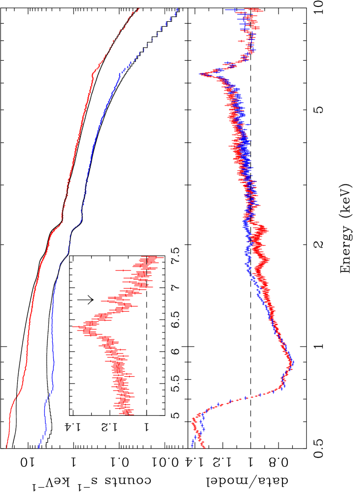
Figure 1: Top panel: EPIC pn (red) and combined MOS1+MOS2 (blue) spectra, Bottom panel: Ratio of data to a power-law model joining the 2.5–3 keV data and 7.5–10 keV data (cf. Fig. 1 of Fabian et al. 2002a). As this is not a realistic model for the continuum the residuals should be considered merely as representative of the spectral complexity. The data from the two instruments obviously show slightly different spectral details. The inset panel shows the pn residuals around the iron line region with the $\sim 6.9$ keV feature marked.

Fig. 1 shows the time-averaged EPIC pn and MOS spectra for the entire dataset compared to a simple power-law model fitted between 2.5–3.0 keV and 7.5–10.0 keV. The emission feature peaking at 6.4 keV is prominent, as is the absorption below 2 keV. However, as is also clear from this plot, the detailed spectral features revealed by the two detectors are subtly different. As the instruments were operated simultaneously these differences represent differences in the spectral calibration between the MOS and pn. In particular, the pn shows a somewhat steeper spectral slope ($\Gamma=1.97\pm 0.08$ for the pn compared to $\Gamma=1.86\pm 0.15$ for the MOS), a larger excess of emission in the 3.5–5.5 keV band, and obvious sharp features around $\sim 1.8$ keV and $\sim 2.2$ keV. These last two features are most likely associated with the instrumental edges of Si-K at 1.84 keV and Au-M at 2.3 keV. The two spectra also diverge strongly below $\sim 0.6$ keV.

Detailed spectral fits to the 2.5–10.0 keV spectrum were presented in Fabian et al. (2002a) based on the MOS data only. These gave a more conservative estimate of the strength and breadth of the broad iron line than the pn data. The greater excess in the pn data in the 3.5–5.5 keV band leads to an apparently stronger line with a significantly stronger red wing. Fitting Model 3 of Fabian et al. (2002a) to the 2.5–10 keV pn spectrum gave a good fit ($\chi^{2}=1310.9$ for $1492$ degrees of freedom, $dof$) with the following parameters: continuum slope $\Gamma=2.02\pm 0.01$, disc inclination $i=27.5\pm 0.9$ deg, inner radius $r_{\rm in}=1.95\pm 0.03r_{\rm g}$, break radius $r_{\rm br}=6.1_{-0.5}^{+0.8}r_{\rm g}$, inner emissivity index $q_{\rm in}=5.5\pm 0.3$, outer emissivity index $q_{\rm out}=2.7\pm 0.1$ and a line equivalent with of $EW=685_{-32}^{+50}$ eV. The equivalent width of the possible $\sim 6.9$ keV emission line is $EW=17\pm 3$ eV.

It should be noted that while the above calibration problems remain with the EPIC spectral responses, it is not clear whether the MOS or the pn data give a more accurate description of the shape of the broad iron line. However, while the absolute values of best-fitting model parameters are sensitive to detector-dependent calibration, the spectral variability characteristics should be, to first order at least, independent of these problems. Therefore, the pn data are used for the purposes of the spectral variability analysis below as they have the highest signal-to-noise ratio. It should be noted that while the form of the spectral variability should be calibration-independent, the exact details of any spectral models will remain sensitive to the calibration uncertainties outlined above.

2.2 Spectral variability

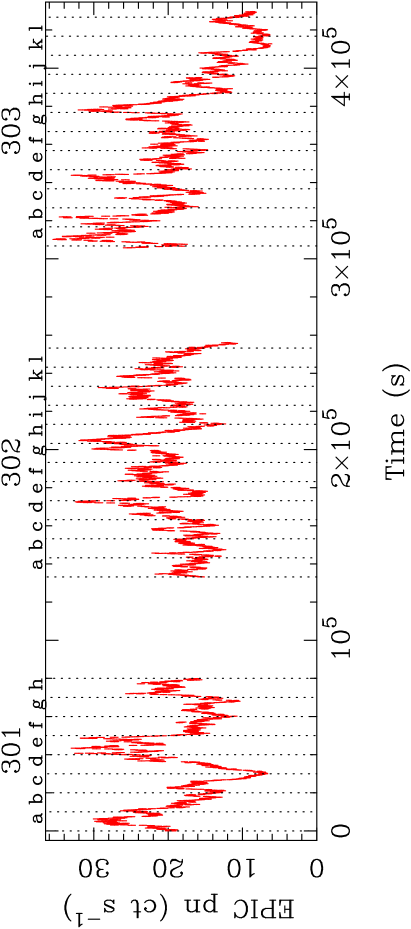
Figure 2: EPIC pn light curve (0.2–10 keV) showing the 10 ks intervals flux discussed in the text. (This light curve has not been corrected for the live-time of the pn camera in small-window mode, which is just a scaling factor.)

2.2.1 The difference spectrum

In this section the two-component model discussed in Shih et al. (2002) is applied to spectra obtained from the XMM-Newton observation. If the spectrum can be broken into two distinct emission components then the observed spectrum during any given time interval, accounting for the effects of absorption, can be written as $S=A\times(N_{1}s_{1}+N_{2}s_{2})$, where $s_{1}$ and $s_{2}$ represent the spectra of the two emission components, $N_{1}$ and $N_{2}$ are their normalisations, respectively, and $A$ gives the absorption profile.

Shih et al. (2002) found that such a model adequately described the spectral variability observed in MCG–6-30-15 by ASCA, with one component having a constant flux while the other varied only in normalisation. If the spectral variability can indeed be described in terms of a variable emission component and another component that remains constant (or, at least, varies very little on the timescales of interest) then it becomes possible to examine the absorption profile using the spectral variability. The difference between two spectra that differ significantly in flux (different $N_{1}$ but identical $N_{2}$) is simply $A\times(N_{\rm 1,high}-N_{\rm 1,low})s_{1}$. The difference spectrum is thus the spectrum of the variable component only, modified by absorption. If the variable spectral component is a power-law, as suggested by Shih et al. (2002), then the difference between two spectra of different fluxes should be a simple power-law modified by (Galactic and intrinsic warm) absorption.

In order to examine this possibility the XMM-Newton observation was divided into $32\times 10$ ks intervals (Fig. 2) from each of which spectra were obtained. The lowest-flux spectrum is from interval 303:k. A high-flux spectrum was extracted from the first 80 ksec of data from this revolution (303:a–h). The average count rate during the high-flux interval is $32.6$ ct s^-1 and during the low-flux interval the count rate is $13.5$ ct s^-1 (after correcting for the live-time of the pn camera in small-window mode). Subtracting the two spectra (i.e. high$-$low), accounting for the difference in exposure times, gives the difference spectrum shown in Fig. 3.

2.2.2 A simple absorption model

Across the 3–10 keV band the difference spectrum is well fitted by a power-law, with photon index $\Gamma=2.11\pm 0.05$. The strong, broad iron line, while clear in both the high- and low-flux spectra when examined separately, is not apparent in the difference spectrum. The iron line flux must be very similar in these two spectra, even though the total (i.e. continuum) flux differs by a factor of about 2 above 7 keV. This then implies a very strong line equivalent width during the low-flux interval.

Extrapolating the power-law model to 0.5 keV reveals the attenuation spectrum of the source (Fig. 3). The warm absorber is clear as the large drop above $\sim 0.7$ keV which recovers by about $2$ keV, and the Galactic absorption mostly accounts for the decrease at lower energies. These features can be accounted for using a very simple absorption model (similar to that used to model ASCA data of the source; Otani et al 1996) comprising a power-law modified by absorption from neutral gas of column density $N_{\rm H}=3.4\pm 0.4\times 10^{20}$ cm^-2, explained by the Galactic column density ($4.06\times 10^{20}$ cm^-2; Elvis, Lockman & Wilkes 1989), together with two warm absorption edges (at $E_{1}=0.72\pm 0.005$ keV of depth $\tau_{2}=0.61\pm 0.03$ and at $E_{2}=0.86\pm 0.01$ keV with depth $\tau_{2}=0.19\pm 0.04$). The obvious candidates for such edges are OVII and OVIII, respectively.

Figure 3: Top panel: The difference spectrum (high$-$low). Bottom panel: Data/model residuals when the difference spectrum is compared to a simple power-law model fitted only above 3 keV (red crosses) and a power-law modified by a simple absorber (green circles).

We note that the above simple absorption model may be adequate for fitting data at CCD resolution above 1 keV but cannot be the whole explanation for data below that energy, where absorption by lines and Unresolved Transition Arrays are expected. The important point for the present work is that there are no major absorption features associated with iron-K, i.e. above 7 keV, nor with Si, S etc between 2–4 keV. The broad iron emission line is not strongly affected by any absorption features. Very similar results are obtained if the absolute minimum, 11 ks, spectrum from within intervals 303:k and l is used. Note that these results depend on the absorption not varying, which is consistent with the rms variability spectrum (Fabian et al 2002a) showing no edges.

2.2.3 The low-flux spectrum

The absorption model derived above was then applied to the spectrum obtained from the low-flux interval. Fitting this spectrum with a power-law, and including the absorption as described above, reveals the very strong iron emission line and an excess of emission below $\sim 1.5$ keV (Fig. 4).

The iron line can be modelled by a LAOR profile (Laor 1991) with a high equivalent width ($EW=1.4$ keV) extending into an inner radius of $1.8r_{\rm g}$ with an emissivity profile index of $3.3\pm 0.3$. The spectrum can also be fitted reasonably well with the constant density ionised disc model of Ross, Young & Fabian (1999), when relativistic blurring is included (again using a broken emissivity law). The model used included three times solar abundances and the best-fitting ionisation parameter was $\xi=10$, with the reflection component dominating over the power-law ($R=5.5$). We hereafter refer to this spectral model as the Reflection-Dominated Component (RDC) .

Figure 4: From top to bottom the panels show: a) Data/model ratio plot from fitting the lowest 10 ks flux spectrum with a power-law between 2–3 keV and 7.5–10.0  keV (including the effects of absorption as derived from the difference spectrum); b) $EF_{E}$ model spectrum including relativistic blurring and absorption effects; c) the intrinsic model spectrum (note lines due to OVIII and OVII below 0.7 keV); and d) the data/model ratio of the best fitting model in the 1–10 keV band extended down to 0.5 keV. The drop in the ratio below 0.6 keV can be removed with the addition of another absorption component.

2.2.4 Fitting the whole light curve

We now extend the study of the simple, absorbed, two-component model to the whole dataset. A model consisting of the simple absorption model from Section 2.2.2 applied to the best-fitting RDC and a Power-Law Component (PLC), with all parameters apart from the normalizations and PLC photon index fixed, was then fitted to all 32 spectra over the energy band 1–10 keV.

Figure 5: Top panel: Photon index $\Gamma$ of the PLC plotted versus the normalization of the PLC. Bottom panel: Normalization of the RDC plotted against the PLC normalization.

The results are shown in Fig. 5. All fits gave acceptable values of $\chi^{2}$. The photon index $\Gamma$ of the PLC is seen to lie between 2 and 2.3 for most of the spectra. The deviant results occur when the PLC normalization is low and disappear if the fit is made over the 2–10 keV band. It is possible that there are small changes in the absorption when the flux is low. The RDC normalization is approximately constant and shows variations of up to $\pm 25$ per cent, with the variations showing no obvious correlation with other parameters.

3 Interpretation

We have shown that the spectral variability of MCG–6-30-15, on timescales of 10 ks, is accounted for by an almost constant reflection-dominated component together with a highly variable power-law component, which has an almost constant photon index, supporting the model of Shih et al (2001). We now attempt to interpret the source using a two component RDC plus PLC model. An alternative interpretation, in which the line is progressively ionized and weakened as the source brightens, is presented and discussed by Ballantyne, Vaughan & Fabian (2002).

Explaining the constant emission component provides us with a significant challenge. It appears to be mostly due to reflection. However it is not simply due to reflection of the observed power-law component since that repeatedly varies by factors of two or more on short timescales (but not shorter than the inferred emission region size, if it is indeed only a few $r_{\rm g}$). In other words the RDC and PLC appear to be separate. Since however both show the effects of the warm absorber they must originate in a similar location to within the dimensions of the warm absorber (probably less than 1 pc). As the iron line in the RDC indicates emission peaking at only a few gravitational radii we shall henceforth assume that this is indeed where that component originates. We then have to explain why so little of the continuum which causes the line is observed and why the power-law continuum we do see does not seem to have any associated reflection.

We are driven to consider that the intrinsic X-ray emission is anisotropic, so that the reflection component is a smoothed average of many variable power-law components, most of which do not illuminate our line of sight. This could be due to source geometry, relativistic beaming of the emitters, or to the general relativistic bending of light expected from an emission region so close to the black hole. We now address each of these in turn.

3.1 Geometrical effects

As discussed by Fabian et al. (2002b) in the case of 1H 0707–495, the surface of the disc could be corrugated. If the continuum is emitted close to the surface within the corrugations then it could show large apparent variability as part of it disappears within a corrugation. The reflected component could be strong, since we are only seeing part of the intrinsic PLC (and multiple reflection may operate; Ross et al. 2002), and be approximately constant.

3.2 Intrinsic beaming

If the emitting region, or the emitting electrons, are relativistic, then the emission can be beamed. We may see variations as beams from different regions or populations of electrons sweep our line of sight. Reflection from the disc however responds to the average of many beams sweeping over it. Note that if the particles are relativistic then the reflection can be strong due to the intrinsic anisotropy of the inverse-Compton process (Ghisellini et al. 1991).

3.3 General relativistic effects

If we accept the evidence from the line shape the the emission peaks at say $2r_{\rm g}$, then the returning radiation (Cunninham 1975) will be very important (see also Martocchia et al. 2002; Dabrowski et al. 1997). An observer on the disc at that radius would see much of the Sky covered by disc, due to gravitational light bending. The reflection is therefore strong and dominated by the average PLC emission from the opposite side of the disc. The PLC which we see will be dominated by the approaching side, perhaps associated with the plunge region just within the marginally stable orbit (Krolik 1999, Agol & Krolik 2000). This will be a much smaller region, also Doppler boosted, than that to which the reflection responds. If its height varies with time then so will the flux of the PLC, whereas the RDC will see a much more constant illumination and so vary little (see Dabrowski & Lasenby 2001, Fig. 12, for the expected variation in equivalent width, dominated by changes in height of the PLC). The appearance of the PLC and RDC are therefore essentially decoupled, as required.

4 Discussion

The iron line in MCG–6-30-15 appears to indicate an extreme disc around a spinning black hole. We have proposed several explanations for the apparent constancy of the RDC and distinguishing between them is not simple. General relativistic effects ought however to be important if much of the emission originates at about $2r_{\rm g}$. They do provide a simple explanation in which small changes in the height of the power-law emission region lead to large changes in the observed flux as a consequence of gravitational light bending; much of the flux is bent onto the disk giving a strong, almost constant, reflection component. This model will be pursued in detail elsewhere.

If instead the emission is anisotropic due to relativistic beaming, then the PLC might extend as a power-law to high energies, perhaps above 500 keV as seen in the hard tail in the soft state of Cygnus X-1.

In summary, we find that the spectrum of MCG–6-30-15 is well represented by the sum of an almost constant reflection-dominated component and a highly variable power-law component. We emphasise that this is only an approximation to the spectral variability as it does not account for the observed changes in the power-spectral density with energy, nor the hard lags (Vaughan et al 2002). Acting on both is a warm absorber, which above 1 keV is relatively simple and dominated by highly-ionized oxygen. Provided that the emission predominantly originates from about $2r_{\rm g}$, then the strengths of the components and their behaviour are accounted from by strong gravtiational light-bending. The black hole in this case is presumably spinning rapidly.

Strong broad iron lines in active galactic nuclei may require the central black hole to have a high spin in order that returning radiation creates a strong reflection component. If the rapid variability in MCG–6-30-15 is in part due to strong light-bending amplifying small changes in source height, then the similarity with the timing behaviour of the soft state of Cygnus X-1 (Vaughan, Fabian & Nandra 2002) suggests that it too may be rapidly spinning. Further extrapolation to the variability of many Narrow-Line Seyfert 1 galaxies (e.g. Boller et al 1997) is also interesting.

References

- [1] Agol E., Krolik, J.H., 2000, ApJ, 528, 161
- [2] Arnaud, K. 1996, in: Astronomical Data Analysis Software and Systems, Jacoby, G., Barnes, J., eds., ASP Conf. Series Vol. 101, p17
- [3] Ballantyne D.R., Vaughan S.A., Fabian A.C., 2002, MNRAS submitted
- [4] Boller T., Brandt W.N., Fabian A.C., Fink H.H., 1997, MNRAS, 289, 393
- [5] Cunningham, C. T. 1975, ApJ, 202, 788
- [6] Dabrowski, Y., Fabian, A. C., Iwasawa, K., Lasenby, A. N., Reynolds, C. S. 1997, MNRAS, 288, L11
- [7] Dabrowski, Y., Lasenby, A. N., 2001, MNRAS,
- [8] Dickey J. M., Lockman F. J. 1990, ARA&A 28, 215
- [9] Fabian, A. C., Rees, M. J., Stella, L., White, N. E., 1989, MNRAS, 238, 729
- [10] Fabian, A. C. et al. 2002a, MNRAS, 335, L1
- [11] Fabian, A. C., Ballantyne, D. R., Merloni, A., Vaughan, S., Iwasawa, K., Boller, Th. 2002b, MNRAS, 331, L35
- [12] Ghisellini, G., George, I. M., Fabian, A. C., Done, C. 1991, MNRAS, 248, 14
- [13] Iwasawa, K., et al. 1996, MNRAS, 282, 1038
- [14] Iwasawa, K., Fabian, A. C., Young, A. J., Inoue, H., Matsumoto, C., 1999, MNRAS, 306, L19
- [15] Krolik, J.H., 1999, ApJ, 515, 73
- [16] Laor, A., 1991, ApJ, 376, 90
- [17] Martocchia, A., Matt, G., Karas, V. 2002, A&A, 383, L23
- [18] Matt, G., Perola, G. C. 1992, MNRAS, 259, 433
- [19] Otani C., et al., 1996, PASJ, 48, 211
- [20] Reynolds, C. S. 2000, ApJ, 533, 811
- [21] Reynolds, C. S., Heinz, S., Fabian A.C., Begelman M.C., 1999, ApJ, 521, 99
- [22] Ross, R. R., Young, A. J., Fabian A. C. 1999, MNRAS, 306, 461
- [23] Ross, R. R., Fabian A.C., Ballantyne D.R., 2002, MNRAS, 336, 315
- [24] Shih, D. C., Iwasawa, K., Fabian, A. C. 2002, MNRAS, 333, 687
- [25] Stella, L. 1990, Nature, 344, 747
- [26] Tanaka, Y., et al. 1995, Nature, 375, 659
- [27] Vaughan, S., Edelson, R. 2001, ApJ, 548, 694
- [28] Vaughan, S., Fabian, A. C,. Nandra, K. 2002, MNRAS, in press
- [29] Wilms, J., Reynolds, C. S., Begelman, M. C., Reeves, J., Molendi, S., Staubert, R., Kendziorra, E., 2001, MNRAS, 328, L27