Black hole growth and activity in a $\Lambda$CDM Universe

Abstract

The observed properties of supermassive black holes suggest a fundamental link between their assembly and the formation of their host spheroids. We model the growth and activity of black holes in galaxies using $\Lambda$CDM cosmological hydrodynamic simulations by following the evolution of the baryonic mass component in galaxy potential wells. We find that the observed steep relation between black hole mass and spheroid velocity dispersion, $M_{\rm BH}\propto\sigma^{4}$, is reproduced if the gas mass in bulges is linearly proportional to the black hole mass. To a good approximation, this is equivalent to assuming the conversion of a fixed fraction of gas mass into black hole mass. In this model, star formation and supernova feedback in the gas are sufficient for regulating and limiting the growth of the central black hole and of its gas supply. Black hole growth saturates because of the competition with star-formation and in particular feedback, both of which determine the gas fraction available for accretion. Unless other processes also operate, we predict that the $M_{\rm BH}-\sigma$ relation is not set in primordial structures but is fully established at low redshifts, $z\mathrel{\hbox to0.0pt{\lower 3.0pt\hbox{$\sim$}\hss}\raise 2.0pt\hbox{$<$}}2$, and is shallower at earlier times. Once this relation is established we find that that central black hole masses are related to their dark matter halos simply via $M_{\rm BH}\mathrel{\hbox to0.0pt{\lower 3.0pt\hbox{$\sim$}\hss}\raise 2.0pt\hbox{$\propto$}}M_{\rm DM}^{4/3}$. We assume that galaxies undergo a quasar phase with a typical lifetime, $t_{Q}\sim 2\times 10^{7}$ yr, the only free parameter of the model, and show that star-formation regulated depletion of gas in spheroids is sufficient to explain, for the most part, the decrease of the quasar population at redshift $z<3$ in the optical blue band. However, with the simplest assumption of a redshift independent quasar lifetime, the model slightly overpredicts optical quasar numbers at high redshifts although it yields the observed evolution of number density of X-ray faint quasars over the whole redshift range $1<z<6$. Finally, we find that the majority of black hole mass is assembled in galaxies by $z\sim 3$ and that the black hole accretion rate density peaks in rough correspondence to the star formation rate density at $z\sim 4-5$.

1. Introduction

Recent dynamical studies indicate that supermassive black holes reside at the centers of most nearby galaxies (e.g., Kormendy & Richstone 1995; Richstone et al. 1998; Kormendy & Gebhardt 2001). The evidence indicates that the mass of the central black hole is correlated with the bulge luminosity (e.g., Magorrian et al. 1998) and even more tightly with the velocity dispersion of its host bulge, where it is found that $M_{\rm BH}\propto\sigma^{~{}4}$ (Tremaine et al. 2002; Ferrarese & Merritt 2000; Merritt & Ferrarese 2001; Gebhardt et al. 2000). The tight relation between the mass of the black holes and the gravitational potential well that hosts them strengthens the theoretical arguments that there is a fundamental link between the assembly of black holes and the formation of spheroids in galaxy halos. In addition, the locally inferred black hole mass density appears to be broadly consistent with the density accreted during the quasar phase (e.g; Soltan 1982; Fabian & Iwasawa 1999; Yu & Tremaine 2002) further supporting the idea that the nuclear activity, the growth of the black holes and spheroid formation are all closely linked.

It is not yet determined what fundamental physical process is responsible for establishing the observed $M_{\rm BH}-\sigma$ relation or what drives the strong evolution of quasars at low redshifts. Suggestions for the $M_{\rm BH}-\sigma$ dependence have appealed to strong feedback due to quasar outflows on the protogalactic gas reservoir (e.g., Silk & Rees 1998); to capture of stars following protogalactic collapse (Adams, Graff & Richstone 2001) and to star formation regulated black hole growth (Burkert & Silk 2001). Models within the context of cold dark matter (CDM) cosmologies, in which the black hole growth is linked to the growth of galactic halos and activity is triggered during major mergers often make use of the observed $M_{\rm BH}-\sigma$ relation (e.g., Wyithe & Loeb 2002; Volonteri, Haardt & Madau 2002 and references therein), or derive it dependent on some additional model assumptions (e.g., Kauffmann & Haehnelt 2000; Haehnelt & Kauffmann 2001).

In the commonly adopted merging scenario for the formation of spheroids, it is well established that black hole masses resulting from the coalescence of progenitor black holes fall short of the measured values (e.g., Ciotti & van Albada 2001). A large fraction of the black hole mass must therefore have been accreted, presumably as gas. At the same time, the gas present in the central region of spheroids must provide the gas supply that will eventually be accreted onto the black hole. In the simplest scenario the growth of the central black hole and the amount of fuel available (hence the black hole activity) should therefore be tied to the evolution of the gas component in galaxies.

In this paper we investigate the growth and activity of black holes in bulges and attempt to look for correlations with the large scale properties of galaxies that match those of the observed black holes at their centers. We use $\Lambda$CDM cosmological hydrodynamic simulations to follow the evolution of the baryonic mass in the potential wells of galaxies. The simulations (Springel & Hernquist 2003a,b) include a new prescription for star formation and feedback processes within the interstellar medium which has been shown to produce a numerically converged prediction for the cosmic star formation history. Our aim is to trace from early times the gas fraction available for accretion and hence for the growth and fueling of black holes in competition with star formation and spheroid growth. This should allow us to determine directly to what extent both the $M_{\rm BH}-\sigma$ relation for black holes, and the decline of quasars at low redshifts, are established through self-regulated star formation processes in the popular cold dark matter cosmogonies.

In §2 we briefly describe the simulations and our analysis. In §3 and §4 we present our results for the $M_{\rm BH}-\sigma$ relation and our predictions for the luminosity function and space density evolution of quasars. We discuss further implications of our results in §5. In this paper we will limit ourselves to redshifts $z<7$ where the quasar luminosity function has been measured. In future work we plan to extend our analysis to make predictions for the QSO population up to very high redshifts.

2. Simulations and analysis

Throughout, we shall use a set of cosmological simulations for a $\Lambda$CDM model, with $\Omega_{\Lambda}=0.7$, $\Omega_{\rm m}=0.3$, baryon density $\Omega_{\rm b}=0.04$, a Hubble constant $H_{0}=100h\hbox{$\hbox{${\rm\thinspace km}{\rm\thinspace s}^{-1}\,$}{\rm\thinspace Mpc}^{-1}$}$ (with $h=0.7$) and a scale-invariant primordial power spectrum with index $n=1$, normalized to the abundance of rich galaxy clusters at the present day ($\sigma_{8}=0.9$). We here briefly summarize the main features of our simulation methodology and refer to Springel & Hernquist (2003a,b) for a more detailed description.

Besides self-gravity of baryons and collisionless dark matter, the simulations follow hydrodynamical shocks, and include radiative heating and cooling processes of a primordial mix of helium and hydrogen, subject to a spatially uniform, time-dependent UV background (see, e.g., Katz et al. 1996, Davé et al. 1999). The dark matter and gas are both represented computationally by particles. In the case of the gas, we use a smoothed particle hydrodynamics (SPH) treatment (e.g., Springel et al. 2001) in its entropy formulation (Springel & Hernquist 2002).

In our numerical model, we assume that collapsed gas at very high overdensity becomes available for star formation, which in turn creates a complex multi-phase interstellar medium (ISM). We use a sub-resolution model to describe the structure and dynamics of the ISM on unresolved scales. In this model, star formation is assumed to occur in cold clouds that form by thermal instability out of a hot ambient medium, which is heated by supernova explosions. These supernovae also evaporate clouds, thereby establishing a tight self-regulation cycle for star formation in the ISM.

Motivated by observational evidence for the ubiquitous presence of strong galactic outflows in actively star-forming galaxies (e.g.; Martin et al. 1999; Heckman et al. 2000) and by the required enrichment of the the interstellar medium (together with the relatively low efficiency of the global star formation) we have also included a phenomenological treatment of galactic winds. In the fiducial parameterization of this process, each star forming region is assumed to drive a wind with a mass outflow rate twice the star formation rate. We then assume that the kinetic energy of the galactic winds is comparable to the total available energy released by the supernovae associated with star formation. This parametrization leads to an initial wind speed in the simulations equal to $484\,{\rm km\,s^{-1}}$. These wind parameters are chosen to be representative of typical properties of the outflows associated with star forming disks (e.g. Martin, 1999). We note that whether or not the wind will escape from a galaxy (as it interacts and entrains infalling gas, shocks the ISM etc.) depends primarily on the depth of the galaxy potential well. For our choice of wind parameters we expect that only those halos with virial temperatures below $10^{6}{\rm\thinspace K}$ have central escape velocities lower than the wind speed and will then lose some baryons in the outflows (c.f. §3.2).

Note that our simulations did not include any prescription for black hole growth when they were run. The gas in our simulated galaxies is therefore only affected by star formation and winds.

In order to resolve the full history of cosmic star formation, Springel & Hernquist (2003a,b) simulated a series of cosmological volumes with sizes ranging from 1$h^{-1}$ Mpc to 100$h^{-1}$ Mpc. For each box size, a series of simulations was computed where the mass resolution was increased systematically in steps of $1.5^{3}$, and the spatial resolution in steps of 1.5.

In this work, we show results mostly from their ‘D-Series’ which employed a periodic box of comoving side length 33.75 $h^{-1}$ Mpc. Within this series, we use the ‘D3’, ‘D4’ and ‘D5’ simulation runs with resolutions of $2\times 144^{3}$, $2\times 216^{3}$ and $2\times 324^{3}$ particles, respectively, corresponding to mass resolutions in the gas of $1.43\times 10^{8}h^{-1}\hbox{$\rm\thinspace M_{\odot}$}$, $4.24\times 10^{7}h^{-1}\hbox{$\rm\thinspace M_{\odot}$}$ and $1.26\times 10^{7}h^{-1}\hbox{$\rm\thinspace M_{\odot}$}$. The spatial resolution of these simulations can be characterized by their gravitational softening lengths, which are equal to 9.38, 6.25, and 4.17 $h^{-1}{\rm\thinspace kpc}$ (in comoving units), respectively. The simulations of the D-Series have only been evolved to a minimum redshift of $z=1$, because at this epoch, their fundamental mode starts to become non-linear. Among the simulation program studied by Springel & Hernquist (2003b), the D-Series constitutes the best compromise between redshift coverage and resolution appropriate for the work here. The analysis of three simulations of different resolution but equal volume allows us to cleanly assess numerical convergence for all the physical quantities we measure, which is a significant advantage of our methodology. For example, Springel & Hernquist (2003b) show that the star formation has fully converged below $z\simeq 6$ in the D5 run, while this is only the case for $z\simeq 5$ in D4, and for $z\simeq 4$ in D3. In general, we therefore expect that progressively higher resolution will also be required to achieve convergence for measurements of other physical quantities related to dissipative processes in the gas. We hence analyze simulation outputs for a set of 10 redshifts, given by $z=7$, $6$, $5$, $4$, $3.5$, $3$, $2.5$, $2$, $1.5$, and $1$.

Note that in this work we attempt to link the large-scale properties of galaxies to those of observed black holes; for this goal it is not important to numerically resolve the properties of the accretion flows close to black holes.

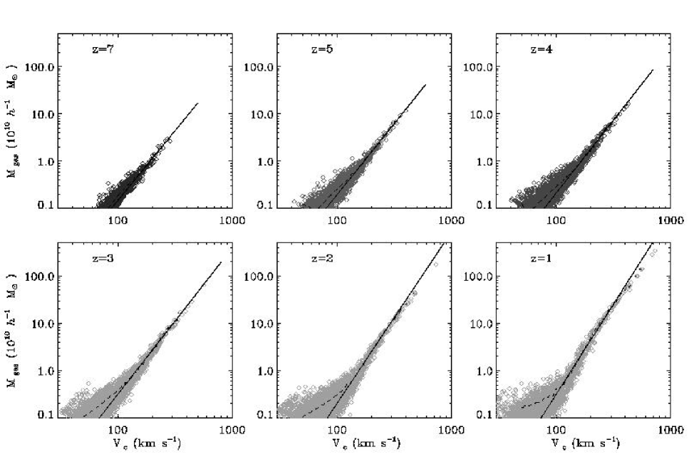
Figure 1.— The evolution from $z=7$ to $z=1$ of total gas mass, $M_{\rm gas}$, versus circular velocity $V_{c}$, for galaxies in the D5 simulation. The dashed line shows the mean relation. The solid line shows a power-law (in log) fit to the points. The power-law index of the fitted line varies from 2.95 at $z=7$ to 3.98 at $z=1$ (see text).

2.1. Galaxy definition

For the galaxy selection we used the Friends-of-Friends (FoF) algorithm to find groups of particles in the various simulation outputs. A linking length of 0.1 times the mean spacing of dark matter particles was used (also equal to $0.1\times 2^{1/3}=0.125$ times the mean spacing of the initial total number of particles). The algorithm was applied to all star, gas and dark matter particles. In choosing the linking length, we have ignored the increase in the total number of particles due to creation of star particles as the simulation evolves. Making allowances for this would change the linking length by about $1.5\%$ in the most extreme case. We discarded groups that contained fewer than 32 particles and also those with either no gas or no star particles. The FoF algorithm was chosen in the interests of simplicity, but we have checked that using another groupfinder such as SKID (e.g., Governato et al. 1997) makes no significant difference to our results.

Figure 2.— The 3D velocity dispersion of star particles, $\sigma$, versus circular velocity, $V_{c}$, of galaxies in the D5 simulation output at $z=1$. The solid line is a linear fit (in log space) to the points.

                 

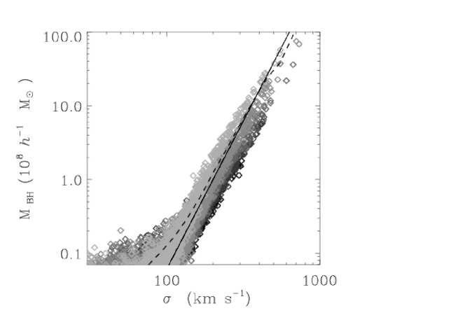
Figure 3.— The relation we obtain between $M_{\rm BH}$ (assumed to be proportional to the total gas mass) and velocity dispersion $\sigma$ of stars for groups in the ‘D5’ simulation. The dashed line shows the mean relation over all redshifts, i.e. for $z=7$, $6$, $5$, $4$, $3.5$, $3$, $2.5$, $2$, $1.5$, and $1$. For comparison, the solid line shows a power-law with a logarithmic slope of 4.

For each redshift output, we obtain a list of halos with their stellar ($M_{\rm star}$), baryonic ($M_{b}=M_{\rm gas}+M_{\rm star}$) and dark matter ($M_{\rm DM}$) mass components, and their positions. The total mass ($M=M_{b}+M_{\rm DM}$) of each galaxy is used to give a measure of its radius and circular velocity. Following Mo & White (2002) and Springel & Hernquist (2003b), we assign a physical radius to a group of mass $M$ according to

$$r_{500}=\left[\frac{GM}{250\Omega_{m}(z)H^{2}(z)}\right]=\frac{1}{1+z}\left[\frac{GM}{250\Omega_{0}H_{0}^{2}}\right]^{1/3},$$ (1)

and a corresponding circular velocity $V_{c}=(GM/r_{500})^{1/2}$, which may be expressed as

$$V_{c}=(1+z)^{1/2}(GM)^{1/3}(250\Omega_{0}H_{0}^{2})^{1/6}.$$ (2)

In these equations, we assumed that the selected groups on average enclose an overdensity of 500 times the background value, which is slightly higher than the canonical value of 200 usually adopted in dark matter only simulations when a linking length of 0.2 is employed. In this way, we compensate for the bias in the measured group masses that arises from the slightly different distributions of gas and dark matter particles on the scale of the ‘virial radius’ $r_{200}$. Within this radius, the gas particles are actually slightly underabundant compared to dark matter particles, such that we effectively select groups at a somewhat higher overdensity contour compared to a corresponding dark matter only simulation. In fact, we have directly compared our measured group masses to an alternative selection that defines groups based on FoF applied to the dark matter only, using the canonical linking length of 0.2, and increasing the final group mass by the enclosed gas and star particles. In this case, the density contrast with respect to the background can be assumed to be 200, and the group mass $M_{200}$ may be defined to represent the ‘virial mass’. We have correlated the two mass definitions using an object-to-object comparison and found very small scatter between the two different selection methods, with the two masses being related by

$$M_{200}\simeq 1.6M,$$ (3)

which can be used to approximately convert the masses we quote in this paper to the virial masses of halos. We will also use the $M_{200}$ catalogues to compare the differences between the baryon fraction in objects selected with the two different methods (see §3.2).

For each galaxy we also directly calculate 3D stellar velocity dispersions, $\sigma$, from the star particles. Finally, we measure the amount of cold gas $M_{\rm cold}$ in galaxies, which we here define to be the mass of actively star-forming cold clouds in the ISM.

3. Cosmological black hole growth

In Figure 1, we plot the gas mass $M_{\rm gas}$ for each individual object selected in the six simulation outputs at redshifts $z=7$, $5$, $4$ , $3$, $2$, and $1$, versus its circular velocity $V_{c}$. The dashed line shows the average relationship traced by the galaxies at the different redshifts and the solid line represents the best power law fit to the objects with $V_{c}\geq 80\hbox{${\rm\thinspace km}{\rm\thinspace s}^{-1}\,$}$. The fit has functional form

$$\log\left(\frac{M_{\rm gas}}{10^{10}h^{-1}\hbox{$\rm\thinspace M_{\odot}$}}\right)=a\log\left(\frac{V_{c}}{200\hbox{${\rm\thinspace km}{\rm\thinspace s}^{-1}\,$}}\right)+b,$$ (4)

where the constants $a$ and $b$ for the six redshifts are $(z=7;2.95,-9.02)$; $(z=5;3.00,-9.02)$; $(z=4;3.08,-9.12)$; $(z=3;3.10,-8.98)$; $(z=2;3.65,-10.2)$; $(z=1;3.98,-10.4)$. Here we do not attempt to assess the significance of the correlations as the sources of scatter in the measurement of $M_{\rm gas}$ cannot be easily quantified (see §3.1); the fitting is merely intended to illustrate the overall evolution of the slope, $a$, that best describes the relation. The most remarkable feature that we note is the steepening of the $M_{\rm gas}-V_{c}$ relation from values $a\sim 3$ at high redshifts, to $a\sim 4$ at $z\mathrel{\hbox to0.0pt{\lower 3.0pt\hbox{$\sim$}\hss}\raise 2.0pt\hbox{$<$}}2$.

We then compare the slopes (in log) of the $M_{\rm gas}-V_{c}$ relation to the most recently revised $M_{\rm BH}-\sigma$ relation from Tremaine et al. (2002)

$$M_{\rm BH}=(1.5\pm 0.2)\times 10^{8}\hbox{$\rm\thinspace M_{\odot}$}\left(\frac{\sigma}{200\hbox{${\rm\thinspace km}{\rm\thinspace s}^{-1}\,$}}\right)^{4.02\pm 0.32}.$$ (5)

(Note that the first published estimates of the slope (in log) of the above relation varied from values $\sim 4.8$; Ferrarese & Merritt (2000); Merritt & Ferrarese (2001); to $\sim 3.75$ Gebhardt et al. (2000), highlighting the difficulty of these measurements). In our lowest redshift output, at $z=1$, the observed slope of the $M_{\rm BH}-\sigma$ relation (Eq. 5) is reproduced well by the $M_{\rm gas}-V_{c}$ relation (Equation 4), suggesting that the slope of Equation 5 is easily explained if $M_{\rm BH}$ is directly proportional to $M_{\rm gas}$ (similar slopes are obtained if we restrict ourselves to $V_{c}\mathrel{\hbox to0.0pt{\lower 3.0pt\hbox{$\sim$}\hss}\raise 2.0pt\hbox{$<$}}400\hbox{${\rm\thinspace km}{\rm\thinspace s}^{-1}\,$}$, consistent with the observed velocity range used to derive the Tremaine et al. 2002 relation). At increasingly higher redshifts, the $M_{\rm gas}-V_{c}$ relation flattens and approaches $M_{\rm gas}\propto V_{c}^{3}$ at $z\sim 7$, as shown by the fitted slopes in Equation (4) and as expected from Equation (2).

To make more direct contact with the observed $M_{\rm BH}-\sigma$ relation and to consider its possible link with the $M_{\rm gas}-V_{c}$ relation in the simulations, we need to consider the relationship between $V_{c}$ and the stellar velocity dispersion $\sigma$, as measured directly from the simulations. The results for the $\sigma-V_{c}$ relationship measured in the simulation are shown in Figure 2; the plot shows the $z=1$ simulation output, although we note that we find no significant temporal evolution in this relation. There is a direct proportionality between $V_{c}$ and $\sigma$, which we fit with the linear relation (in log):

$$\log\;\sigma=1.03\log\;V_{c}-0.32,$$ (6)

shown by the solid line in Figure  2. Because the measurement of $\sigma$ from the star particles is intrinsically much noisier than that of $V_{c}$ (which is effectively a measure of mass), we make use of the relation from (Eq.6) to convert from $V_{c}$ to $\sigma$ in what follows. Using $\sigma$ directly would introduce a significant source of artificial scatter in our simulated $M_{\rm BH}-\sigma$ relation. We note that in future work it might be possible to investigate the scatter about the $M_{\rm BH}-\sigma$ relation provided it is possible to eliminate numerical scatter in the simulated stellar velocity dispersion $\sigma$.

The two relations, $M_{\rm gas}-V_{c}$ and $V_{c}-\sigma$ from the simulations, if compared to the observed $M_{\rm BH}-\sigma$ relation (Eq. 5) suggest that the central black hole mass in galaxy may be simply proportional to the gas mass in galaxies. We hence make this simple ansatz that the black hole mass is proportional to the gas mass, allowing us to plot a predicted relation between $M_{\rm BH}$ and $\sigma$ obtained from the simulations. In Figure 3, we overplot the corresponding data from all the redshift outputs used in Figure 1, resulting in a composite average relation which is shown as a dashed line. Only simulation outputs for the D5 run are included, and we defer a discussion of differences between the D4 and D5 runs to the next section. In order to match the normalization of the observed $M_{\rm BH}-\sigma$ relation (Eq. 5) we associate black hole and gas masses here according to

$$M_{\rm BH}=f\;M_{\rm gas}\sim 0.004h^{-1}M_{\rm gas},$$ (7)

where the solid line in Figure 3 shows Equation 5. Assuming that there is no significant change from $z=1$ to $z=0$, (which we have checked is a good approximation by making use of the larger 100 h^-1 Mpc simulation box in the G-Series; see Springel & Hernquist 2003a) this therefore implies that in the context of our model, the mass of the central black hole in galaxies is consistent with being $\mathrel{\hbox to0.0pt{\lower 3.0pt\hbox{$\sim$}\hss}\raise 2.0pt\hbox{$<$}}1$ per cent of the total gas mass in galaxies.

In this interpretation, the $M_{\rm BH}-\sigma$ relation is not set in primordial structures and maintained through cosmic time; it is established at later times as the growth of black holes is limited by the available gas, in competition with star formation and associated feedback processes like galactic winds. Because both the black hole growth and the change of the amount of available gas occur gradually from high to low redshifts, the resulting correlation does not show large scatter. Note, however, that in this simple model, the high-mass, high-redshift objects are predicted to lie on the right of the main relation. Large samples of intermediate mass objects at $z\mathrel{\hbox to0.0pt{\lower 3.0pt\hbox{$\sim$}\hss}\raise 2.0pt\hbox{$>$}}3$ will be required to determine observationally whether the $M_{\rm BH}-\sigma$ relation is indeed shallower at earlier times, as predicted here. At present the observed $M_{\rm BH}-\sigma$ relation (as shown in Eq. 5) is derived from local objects. For objects at $z=1$ (sixth panel of Fig. 1) the predicted relation is extremely tight.

Note also that given the $\sigma-V_{c}$ relation (Eqs. 6 and  7) from the simulations we find that the black hole mass is related to the dark matter mass of the host galaxy by the relation:

$$\frac{M_{\rm BH}}{10^{8}\hbox{$\rm\thinspace M_{\odot}$}}\sim 0.7\left(\frac{M_{\rm DM}}{10^{12}\hbox{$\rm\thinspace M_{\odot}$}}\right)^{4/3}.$$ (8)

This is broadly consistent with the $M_{\rm BH}-V_{c}$ relation derived by Ferrarese (2002) and Baes et al. (2003), reflecting the fact that the relation in Equation 6 matches the observed correlation between $V_{c}$ and $\sigma$ (Ferrarese 2002; Baes et al. 2003).

3.1. Numerical convergence and scatter

3.1.1 Deviations from a power law

Figures 1 and 3 show that, for small values of $M_{\rm gas}$ and $V_{c}$, the $M_{\rm BH}-\sigma$ relation deviates significantly from a power-law and its scatter is increased. Figure 4 shows the same plot as in Figure 1 but with the D3, D4 and D5 simulations over-plotted at $z=1$ in the top panel, and the D5 and Q5 simulations in the bottom panel. The ‘Q5’ simulation is taken from the Q-Series of Springel & Hernquist (2003b). While Q5 has a smaller cosmological volume of size 10$h^{-1}$ Mpc on a side, its particle number is equal to that of D5, so that the mass resolution in the gas becomes $3.26\times 10^{5}h^{-1}\hbox{$\rm\thinspace M_{\odot}$}$ (a factor of 40 improvement over D5), and the spatial resolution becomes 0.63 $h^{-1}{\rm\thinspace kpc}$ in comoving units.

In the top panel of Figure 4, the average relations for the D3, D4 and D5 runs are shown with the dashed, solid and dot-dashed lines, respectively. The figure shows that both the scatter and the deviation from the $V_{c}^{4}$ relation decrease with increasing resolution of the simulation. This is a result of the fact that close to the resolution limit of each of the simulations, star formation cannot be resolved properly any more, making the measurement of $M_{\rm gas}$ unreliable. For higher resolution simulations, this limit for convergence in $M_{\rm gas}$ moves to lower mass systems.

However, when analyzed in isolation, even for the D5 run it is not clear whether the flattening of the relation at small $V_{c}$ is due to some underlying physical process associated with star formation, or whether it can be fully explained by insufficient resolution. We investigate this further in the bottom panel of Figure 4, where we show a comparison of the measured gas content between the D5 and the Q5 simulations at redshift $z=3$ (this is close to the minimum redshift reached by the Q-Series). Although the number of objects in the high mass range is much reduced in Q5 due its smaller volume, the increased resolution allows us to investigate the $M_{\rm gas}-V_{c}$ relation for much smaller objects. We find almost negligible deviations from the extrapolated power law behavior derived from the D-Series. It is therefore plausible that the $M_{\rm BH}-M_{\rm gas}$ relationship extends to very low $V_{c}$ given sufficient numerical resolution.

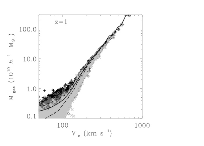
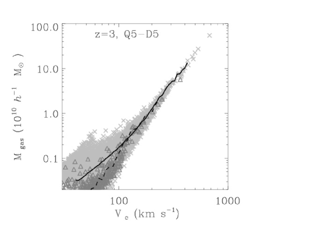
Figure 4.— Convergence study for the measurement of $M_{\rm gas}$. We plot the same quantities as in Figure 1. Top panel: groups extracted from the D3, D4 and D5 simulations at redshift $z=1$ are overplotted with plus signs, triangles and cross symbols, and in shades from dark to light gray, respectively. The dashed line is the average relation in the D3 run, the solid line in D4 and the dash-dotted in D5. The large scatter at small $V_{c}$ is reduced with increased resolution. Bottom panel: We compare here objects in the Q5 (dashed line) and D5 simulations at redshift $z=3$. Thanks to the significantly increased resolution of the Q5 simulation, the scatter is further reduced, showing that it largely arises from resolution effects. However, the small box of Q5 contains only a few high-mass objects.

Determining the extent to which our theoretical relation applies to the low mass range is also relevant in view of recent searches for intermediate mass black holes in globular clusters. The promising detection of a central black hole of $M_{\rm BH}\sim 2\times 10^{3}\hbox{$\rm\thinspace M_{\odot}$}$ in stellar cluster G1 in M31 (Gebhardt, Rich & Ho, 2002) and the ongoing debate on the presence of a similar central object in the globular cluster M15 (Gerssen et al. 2002) seem to be consistent with an extrapolation of the observed $M_{\rm BH}-\sigma$ relation for galaxies, possibly implying a similar formation process for the central black hole.

Figures 1 and 3 also show that for large values of $V_{c}$ the relationship between $M_{\rm gas}$ and $V_{c}$ flattens and almost recovers the power law slope of $\sim 3$ expected from Equation (2). for halos with baryon content consistent with the universal fraction. As we will discuss further in §3.2, stellar feedback with its associated outflows plays a fundamental role in our model for generating the steep decline of gas content towards low-mass halos, but these processes eventually become inefficient for very massive systems, which then recover the universal baryon content.

3.2. The evolution of $M_{\rm gas}$, $M_{\rm star}$ and $M_{\rm cold}$

In order to establish the constant of proportionality $f$ in Equation (7) we need to investigate whether the measurement of $M_{\rm gas}$ has converged for sufficiently large $V_{c}\mathrel{\hbox to0.0pt{\lower 3.0pt\hbox{$\sim$}\hss}\raise 2.0pt\hbox{$>$}}100\hbox{${\rm\thinspace km}{\rm\thinspace s}^{-1}\,$}$. Figure 5 shows the evolution of the total gas, stellar and cold gas (gas subject to star formation) masses, $M_{\rm gas}$, $M_{\rm star}$ and $M_{\rm cold}$ as a function of $z$ at constant circular velocity, $V_{c}=200\hbox{${\rm\thinspace km}{\rm\thinspace s}^{-1}\,$}$. We also include the dark matter component, $M_{\rm DM}$, for comparison. The plot hence shows the evolution of the baryonic (and dark matter) content in typical $L_{\star}$-galaxies. The black symbols and lines are for the D3 simulation, the light gray for the D4 run and the dark gray for the D5 run. For each simulation, the star symbols joined by dot-dashed lines represent $M_{\rm star}$, the triangles joined by the dashed lines $M_{\rm cold}$, and the solid dots joined by the solid lines $M_{\rm gas}$. $M_{\rm DM}$ is shown for the D5 run only, using diamonds connected by a dotted line and rescaled by a factor $\Omega_{b}/\Omega_{\rm DM}=0.153$.

The figure shows that the measurements of $M_{\rm gas}$, $M_{\rm star}$ and $M_{\rm cold}$ at $V_{c}=200\hbox{${\rm\thinspace km}{\rm\thinspace s}^{-1}\,$}$ have converged in the D4 run to good accuracy. In the D3 simulation, the star formation has not fully converged even at this circular velocity; hence $M_{\rm star}$ is lower in the D3 run than in D4 or D5, and $M_{\rm cold}$, in particular, as well as $M_{\rm gas}$ are overestimated.

It is further seen that the ratio $M_{\rm gas}/M_{\rm star}$ is large at high redshifts and approaches values $\mathrel{\hbox to0.0pt{\lower 3.0pt\hbox{$\sim$}\hss}\raise 2.0pt\hbox{$>$}}1$ at redshifts $z\mathrel{\hbox to0.0pt{\lower 3.0pt\hbox{$\sim$}\hss}\raise 2.0pt\hbox{$<$}}3$. The cold gas fraction $M_{\rm cold}/M_{\rm star}$ is also fairly large at high redshift but decreases significantly below $1$ at $z\sim 1$. Interestingly, in this plot we see the overall evolution of the baryon and dark matter mass in galaxies. This will be particularly useful when deriving the evolution of the quasar luminosity function in §4. Here we find that $M_{\rm gas}$ for the circular velocity given, $V_{c}=200\hbox{${\rm\thinspace km}{\rm\thinspace s}^{-1}\,$}$, is a slowly decreasing function of redshift, where we have $M_{\rm gas}\propto(1+z)^{-1/3}$, as opposed to $M_{\rm DM}$, which is a steeper function of redshift, following the relation $M_{\rm DM}\propto(1+z)^{-3/2}$ as expected from Equation (2). Even though gas is both used up by star formation and expelled by galactic outflows, the total mass of gas does not decrease with decreasing redshift but remains nearly constant.

Note that in the Kauffman & Haehnelt (1999) model, in order to explain the small scatter in the $M_{\rm BH}$ - $\sigma$ relation, Haehnelt & Kauffmann (2000) require the cold gas mass of their bulge progenitors to be essentially independent of redshift (where in their model a fixed fraction of the cold gas is assumed to to be accreted by the black holes). Here we find that $M_{\rm cold}$ decreases with redshift and instead the total gas mass $M_{\rm gas}$ is found to be a slowly varying function of redshift. This suggests that the slope of the $M_{\rm BH}$ - $\sigma$ relationship may not be set by the amount of gas that cools and becomes available for star formation, as assumed by Haehnelt & Kauffmann (2000), but rather by the total amount of gas in the galaxies, although it is certainly true that galaxies have higher cold gas fractions at earlier times. In the next section we investigate how star formation and feedback regulate the total amount of gas available for accretion onto central black holes.

Figure 5.— Gas, star, cold gas and dark matter mass components for halos of constant circular velocity $V_{c}=200\hbox{${\rm\thinspace km}{\rm\thinspace s}^{-1}\,$}$ as a function of redshift. The results for the D3 run are shown in black, for D4 in light gray, and for D5 in dark gray. The dark matter mass has been rescaled by a factor $\Omega_{b}/\Omega_{\rm DM}=0.153$ and is shown for comparison only (for D5). Approximate convergence of the various baryonic mass components is already obtained for the resolution of the D4 simulation.

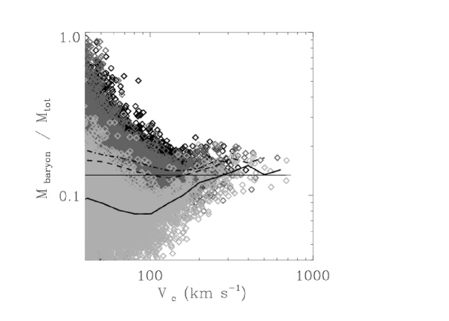
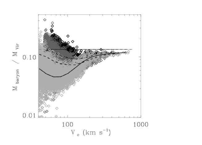
Figure 6.— The baryon mass fraction in galaxies as a function of circular velocity $V_{\rm c}$. Three redshifts, $z=5$, $3$, and $1$, are shown in shades of dark to light gray, and we plot running averages for them in dot-dashed, dashed and solid lines, respectively. The horizontal line shows the baryon fraction $\Omega_{\rm b}/\Omega_{\rm m}$. In the top panel, objects were selected by applying a FoF linking length of 0.1 the initial dark matter particle spacing to all particles, with the total mass in galaxies defined as $M_{\rm tot}=M_{\rm gas}+M_{\rm stars}+M_{\rm DM}$. In the bottom panel, a linking length of 0.2 has been used instead, but was restricted to the set of dark matter particles. Here, the enclosed gas and star particles in each identified group have been added in a separate step (see § 2.1).

3.3. The role of stellar feedback

In Figure 6, we plot the baryonic mass fraction $(M_{\rm gas}+M_{\rm star})/M_{\rm tot}$ in galaxies as a function of $V_{c}$ for the objects in the D5 simulation at the three redshifts $z=5$, $3$, and $1$, overplotted in black, dark gray and light gray, respectively. A running average of the baryon fraction at each redshift is shown as a dash-dotted line for $z=5$, dashed line for $z=3$ and solid line for $z=1$. The solid horizontal line indicates the universal baryon fraction $\Omega_{b}/\Omega_{\rm m}$ expected for our cosmological model. The two panels of the figure show a comparison of the baryon fractions measured for objects selected according to the two group definitions outlined in §2.1. The top panel uses the same definition as in our previous figures, where we applied the FoF algorithm to dark matter, gas and star particles on an equal footing, while in the bottom panel, we selected objects based on dark matter particles only, and then included all enclosed gas and star particles. Based on this comparison, we note that the larger scatter in the top panel at low $V_{c}$ is a consequence of the different group selection methods. In particular, close to the resolution limit our default method is somewhat more prone to occasionally producing measured baryon fractions well above $\Omega_{b}/\Omega_{\rm m}$, as it can happen if the FoF algorithm just picks out the concentrated cold gas and stellar parts of low-mass galaxies, but loses the sparsely sampled dark halo around them. Although this occurs, our method is able to recover the universal baryon fraction at $z=1$ in the simulation more closely (top panel, Fig. 6) than in the bottom panel.

However, more importantly, both plots show that the total baryon mass fraction decreases from intermediate values of $V_{c}$ towards low values, while systems of very large mass remain close to the universal baryon fraction. Furthermore, the strength of the baryonic depletion at low $V_{c}$ increases towards low redshifts.

It is clear that these trends in Figure 6 are a reflection of the same steeping of the $M_{\rm gas}-V_{c}$ relation towards low redshift and low $V_{c}$ that we already observed in Figure 1. However, in this representation the fundamental physical mechanism that drives this evolution is more apparent. In essence, the $M_{\rm gas}-V_{c}$ relation is steepened by the loss of baryons due to strong feedback by galactic winds. These galactic outflows are increasingly more efficient in low mass systems (where resolved; see also Springel & Hernquist 2003b), while for very massive groups, the winds eventually become trapped in deep gravitational potential wells. Note that the measured $M_{\rm gas}$-$V_{c}$ relation indeed flattens for high-mass systems (as shown by Figures 1 and 3), with a transition scale that is consistent with the maximum circular velocity expected to allow an escape of winds from halos in the simulations.

4. Black hole activity

Quasars have long been believed to be powered by the accretion of gas onto supermassive black holes and have been known to evolve very strongly. Their comoving space density increases by nearly two orders of magnitude out to a peak at $z\sim 3$ (e.g., Boyle et al. 2000). Their evolution at higher redshifts is more uncertain although recent observations have begun to constrain the bright end of the luminosity function out to $z\sim 5$ and individual quasars have been detected out to $z=6.28$ (Fan et al. 2001a,b). Here we use our results from §3 to predict the evolution of the number density of bright QSOs from redshift $z=7$ to $z=1$ and compare it with observations.

4.1. Gas accretion history

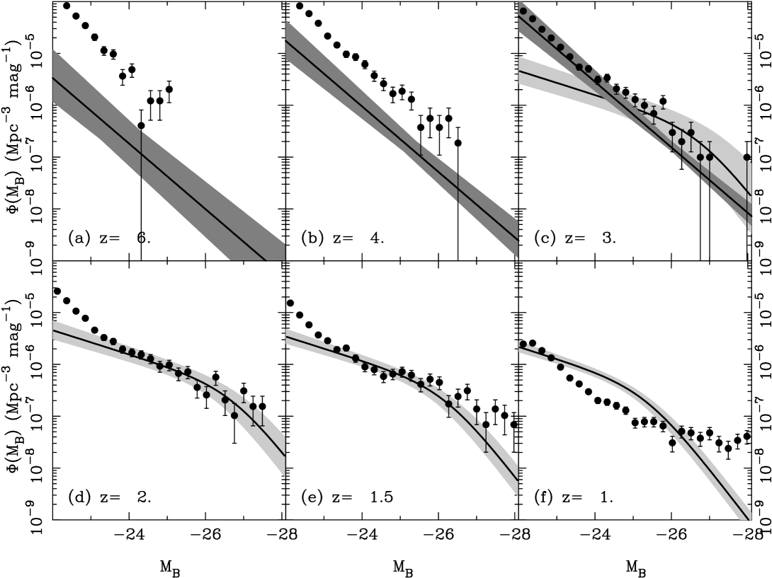
Figure 7.— The $B$-band luminosity function of quasars at various redshifts, as indicated in each panel. The filled circles are the values from our models. Error bars indicate the Poissonian error in the counts. The solid lines and light gray shaded areas at $z=2$, $1.5$, and $1$ show the best fit to the 2dF luminosity function (Boyle et al. 2000). The dark shaded areas and solid lines at $z=6$, $4$, and $3$ give the best fit to the SDSS luminosity function from Fan et al. (2001a,b).

In order to predict black hole luminosities, we need to estimate the amount of gas available for accretion for a given characteristic accretion timescale. In §3 we showed that the mass of the black hole may simply be modeled as a fixed fraction of the total amount of gas in the halo, suggesting that black holes grow primarily by accretion of gas, in which case the amount of accreted mass also depends on star formation and feedback processes.

The small-scale physical processes linked to the growth of black holes, however, do not give us a direct handle for constraining the black hole accretion timescale. Given the lack of any definite prescription or constraint for the quasar lifetime or its evolution, we make the simplest possible assumption and choose the quasar lifetime which is independent of redshift and of order of the Salpeter time $t_{Q}\sim 2\times 10^{7}$ yr. Our choice of $t_{Q}$ is most appropriate for the bright end of the quasar population (for quasars that radiate around the Eddington limit) which is what we concentrate most of our modeling on, as the faint end is dominated by low mass galaxies which may not be fully resolved in the simulations used here (see §3). We note that this choice of timescale is consistent with results of Steidel et al. (2002) who estimated the lifetime of bright quasar activity in a large sample of Lyman-break galaxies at $z\sim 3$ to be $\sim 10^{7}\,{\rm yr}$ and range of quasar lifetimes obtained from quasar clustering constraints ( which generally imply $10^{7}{\rm yr}\mathrel{\hbox to0.0pt{\lower 3.0pt\hbox{$\sim$}\hss}\raise 2.0pt\hbox{$<$}}t_{Q}\mathrel{\hbox to0.0pt{\lower 3.0pt\hbox{$\sim$}\hss}\raise 2.0pt\hbox{$<$}}10^{8}{\rm yr}$; e.g.; Martini & Weinberg 2001). It is interesting to note that a similar timescale, $t_{Q}\sim 2\times 10^{7}$ yr, was also adopted in the models of Sokasian, Abel and Hernquist (2002; 2003) developed to study reionization of HeII and the properties of the ionizing background at intermediate redshifts. In this case, this timescale was shown to match the observations of the HeII Lyman alpha forest and of the H and HeII opacity at $z\sim 2.5-5$.

As we shall see the choice of this parameter is crucial for determining the evolution of the quasar population. For our model, the star formation timescale is $t_{\rm star}\sim$ a few Gyr; hence, we have $t_{Q}<<t_{\rm star}<<H_{0}^{-1}$, consistent with our hypothesis that the overall cosmological change in the environment governs the quasar activity and the duty cycle of quasars increases with redshift.

We assume that all galaxies can undergo a quasar phase and so accrete a fraction of their total gas content. Because, in general, the evolution of the gas mass in galaxies follows an evolution $\mathrel{\hbox to0.0pt{\lower 3.0pt\hbox{$\sim$}\hss}\raise 2.0pt\hbox{$\propto$}}(1+z)^{1/3}$ (i.e.; ’on average’ the gas mass does not go down, but merely does not grow; see Fig. 5), we can assume the black hole growth occurring in the last Hubble time always dominates. Hence, we consider the black hole mass at the time of accretion to be the contemporaneous black hole mass. This simple scenario is then consistent with the approximate condition, $M_{\rm BH}\propto M_{\rm gas}$ relating the total gas and black hole masses.

The bolometric luminosity of a quasar at redshift $z$ is then simply given by

$$L=\eta\hbox{$\dot{M}$}(z)c^{2}\sim\eta\frac{\Delta M_{\rm gas}}{\Delta t}c^{2}\sim\eta fM_{\rm gas}(z)c^{2}/t_{Q},$$ (9)

where we have taken $\Delta M_{\rm gas}(z)\sim fM_{\rm gas}(z)$ with $f=0.4\%$, as suggested by Equation (7); i.e. the average mass accreted is a constant fraction of the total gas mass $M_{\rm gas}$. We adopt the standard value for accretion radiative efficiency of $\eta=10\%$, and assume that every object with a nonzero star formation rate (this discards small-mass objects where star formation is likely not resolved) shines as a quasar for a time $t_{Q}$. The expected number density of active quasars at each redshift is a fraction $f(z_{i})=t_{Q}\times(z_{i+1}-z_{i})/[t_{H}(z_{i})-t_{H}(z_{i+1})]$ where $z_{i}$ and $t_{H}(z_{i})$ are the redshift and Hubble time of simulation output $i$, respectively.

4.2. The evolution of the quasar luminosity function

4.2.1 Optical blue band

We now compare our simple predictions for the luminosity function to observational data. We take a fixed fraction $\epsilon_{B}$ of the bolometric luminosity to be radiated in the blue band. In the $B$-band, the bolometric correction $\epsilon_{B}$, defined as $L=\epsilon_{B}\nu L_{B}$, is about 11.8 (Elvis et al. 1994), where $\nu L_{B}$ is the energy radiated at the central frequency of the $B$-band per unit time per logarithmic interval of frequency. At the peak of its lightcurve the quasar has a $B$-band magnitude

$$M_{B}=37.05-2.5\log({\epsilon_{B}L}),$$ (10)

where $L$ is in units of ${\rm\thinspace erg}{\rm\thinspace s}^{-1}\,$. We place an upper limit on the maximum allowed luminosity of a quasar so that $L$ does not exceed the Eddington luminosity $L_{\rm Edd}$. Note that if accreted gas provides the power, then clearly there cannot be steady fueling at rates that generate $L>L_{\rm Edd}$. With the black hole masses given by Equation (7) a small percentage of objects radiate above $L_{\rm Edd}$.

Figure 7 shows a comparison of our theoretical luminosity functions (LFs) at different redshifts with the most recent determinations of the quasar $B$-band LF from the 2dF QSO Redshift survey ($0.3<z<2.3$; Boyle et al. 2000) and the Sloan Digital Sky Survey SDSS ($3.6<z\mathrel{\hbox to0.0pt{\lower 3.0pt\hbox{$\sim$}\hss}\raise 2.0pt\hbox{$<$}}6$; Fan et al. 2001a). For the 2dF, the luminosity function for $-26<M_{B}<-23$ is described by a double power law with a bright end slope of $\beta_{1}=-3.4$ and a faint end slope of $\beta=-1.5$ (Boyle et al. 2000; Pei 1995). The QSO luminosity function measured by Fan et al. (measured for $-25<M_{1450}<-28$; where $M_{1450}$ is the absolute AB magnitude; see Eq (5) in Fan et al. 2001a for the relation between $M_{B}$ and $M_{1450}$) gives a flatter bright-end slope ($\beta_{1}=-2.5$). For the luminosity function at $z=3$, we plot both these functions, one extrapolated from higher redshifts, the other from lower redshifts.

Our simple model reproduces the luminosity function of optically selected quasars in the redshift range $4\mathrel{\hbox to0.0pt{\lower 3.0pt\hbox{$\sim$}\hss}\raise 2.0pt\hbox{$<$}}z\mathrel{\hbox to0.0pt{\lower 3.0pt\hbox{$\sim$}\hss}\raise 2.0pt\hbox{$<$}}1.5$ reasonably well. The overall turnover of the space density of quasar at low redshifts ($z\mathrel{\hbox to0.0pt{\lower 3.0pt\hbox{$\sim$}\hss}\raise 2.0pt\hbox{$<$}}3$) is also reproduced with some overestimate of the number of bright quasars at $z=1$. The slope of the LF at redshifts higher than $z\mathrel{\hbox to0.0pt{\lower 3.0pt\hbox{$\sim$}\hss}\raise 2.0pt\hbox{$>$}}4$ matches the steep value found by Fan et al. (2001a). However, the model at this high redshifts predicts a larger numbers of quasars (both bright and faint) with respect to observations (and their extrapolation to faint magnitudes $M_{B}\mathrel{\hbox to0.0pt{\lower 3.0pt\hbox{$\sim$}\hss}\raise 2.0pt\hbox{$>$}}-25$). At redshifts $z=3$ and $2$, the bright end of the luminosity function flattens in accordance with the observations by Boyle et al. (2000) but remains too flat at $z=1$, leading to an overestimate of the number of bright quasars at these redshifts.

In the top panel of Figure 8, we show the evolution of the space density of bright quasars with luminosity $M_{B}<-26$ as a function of redshift. In this plot, we add as open symbols data from the Warren, Hewett, & Osmer survey (1994; hereafter WHO) in the redshift range $2<z<4.5$, and from Hartwick & Shade (1990) in the range $0.1<z<3.3$, respectively (also summarized in Pei 1995). The dotted line is a fit to the Schmidt, Schneider & Gunn survey (1995; SSG). The Fan et al. (2001a,b) data is shown with solid dots, while our theoretical prediction is shown using solid symbols joined by a solid line. Although this measurement is quite noisy as a result of a relatively small simulation box, the overall evolution of the comoving number density of quasars is reproduced reasonably well by the model. Note that because of our limited box size no objects can be found massive enough to contribute to the luminosity function at $M_{B}<-26$ for $z>5$. As we shall discuss in §4.2.2 , at high redshifts, black hole accretion follows the growth of structure; to a good approximation our prediction at higher redshifts should thus follow the extrapolation from lower redshifts. Because of the small number of objects and the very sharp decrease in the quasar counts for objects brighter than $-26$ our results are very sensitive to the model parameter $t_{Q}$. In order to get a more robust comparison we compare our results to recent constraints on quasar number counts derived from recent Chandra X-ray observations which probe quasars of more intermediate luminosity.

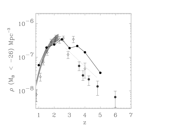
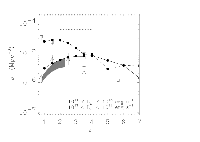
Figure 8.— Top: The evolution of the space density of quasars with $M_{\rm B}<-26$. Our model is shown by the solid circles joined by the thick solid lines. The model is for $t_{Q}=2\times 10^{7}{\rm\thinspace yr}$. The dotted line is a fit to the SSG survey in the redshift range $2.75<z<4.75$. The open squares show a compilation from Pei (1995) derived from the WHO and HS surveys. The filled circles are the SDSS points derived by Fan et al. (2001a,b). The shaded area at low redshift is the best fit model from the 2dF survey by Boyle et al. (2000). Bottom: The evolution of space density of quasar in the $2-8{\rm\thinspace keV}$ X-ray energy band. The data are from recent Chandra observations by Cowie et al. (2003); Barger et al. (2003). The open squares represent the quasar number density of sources with $10^{43}<L_{x}<10^{44}\hbox{${\rm\thinspace erg}{\rm\thinspace s}^{-1}\,$}$, and the open triangle the number density of sources with $10^{44}<L_{x}<10^{45}\hbox{${\rm\thinspace erg}{\rm\thinspace s}^{-1}\,$}$. The dotted bars show upper limits. The solid and dashed lines show our model in these luminosity ranges using with $t_{Q}=2\times 10^{7}{\rm\thinspace yr}$ and $t_{Q}=10^{7}{\rm\thinspace yr}$ respectively.

4.2.2 X-ray band

The bottom panel of Figure 8 shows the redshift evolution of the comoving number density of quasar in the $2-8{\rm\thinspace keV}$ band compared to the recent Chandra observations (Cowie et al. 2003; Barger et al. 2003). We plot our model with solid dots joined by a dashed line and a solid line for two observed luminosity ranges $10^{43}<L_{x}<10^{44}\hbox{${\rm\thinspace erg}{\rm\thinspace s}^{-1}\,$}$ and $10^{43}<L_{x}<10^{44}\hbox{${\rm\thinspace erg}{\rm\thinspace s}^{-1}\,$}$ respectively. We take $L_{x,2-8{\rm\thinspace keV}}\sim 0.03L$ where $L$ is the bolometric luminosity given in Equation 9. This relation seems to be roughly valid for all type of AGN (Elvis et al. 1994). For the higher luminosity range we take $t_{Q}=2\times 10^{7}{\rm\thinspace yr}$ (as in §4.2.1), whereas for the lower luminosity range the quasar timescale is a factor of 2 smaller, $t_{Q}=1\times 10^{7}{\rm\thinspace yr}$, as this seems to describe better the overall evolution of these objects. Overall, we find the model to agree pretty well with the current constraints from the X-ray band if we allow a small, mass dependent variation of the typical accretion timescale. This again emphasizes the strong dependence of our predictions on this parameter.

4.2.3 Dust, obscured AGN, low-radiative efficiency

Observations indicate that the comoving number density of quasars peaks at $z\sim 3$ and drops abruptly by a factor of 20 from redshift $z\sim 2$ to $z\sim 5$. Our predicted number density lies closer to an extrapolation of the low redshift luminosity function (e.g., Boyle et al. 2000), implying a perhaps less rapid evolution at high redshifts. From the observational point of view, there is still some uncertainty concerning the recent high-redshift results as a result of a number of potentially very important systematic biases (see e.g., Pei 1995; Fan et al. 2001a). Surveys at high redshifts still suffer from incompleteness, uncertainties in the K-corrections (when compared to low redshifts) and in particular from the possibility that a large number of quasars are not detectable in optical surveys as a result of dust extinction.

The tendency to overestimate the number of bright quasars at $z\mathrel{\hbox to0.0pt{\lower 3.0pt\hbox{$\sim$}\hss}\raise 2.0pt\hbox{$<$}}1$ in our model may also be less severe given the recent Chandra results, which imply the presence of a substantial population of optically obscured luminous AGNs at low redshifts (e.g., Rosati et al. 2002; Barger et al. 2001). This would help to reduce the discrepancy. We also note that there is significant evidence from Chandra observations of nearby galactic nuclei indicating that the gas supply onto their central black holes far exceeds their luminosity outputs, implying that the radiative efficiency $\eta$ of nearby supermassive black holes may be a lot lower than the canonical value of $\eta=0.1$ we have taken (e.g., the case of M87; Di Matteo et al. 2003; our Galactic Center, Baganoff et al. 2002; Narayan 2002).

In summary, we have shown that the evolution of the gas supply via star formation and feedback can, for the most part and without the introduction of any additional parameters, reproduce the turnover in the comoving number density of quasars at $z<3$. We obtain an improved agreement with observations with respect to previous models in which the evolution of the luminosity function is predicted within the context of hierarchical build-up of the dark halos through merger trees (e.g., Kauffmann & Haehnelt 2000; Cattaneo 2000; Volonteri et al. 2002; Hatziminaoglou et al. 2002). However other factors such as obscuration or change in radiative efficiency or other feedback processes (e.g.; due to radio jets) may still play some role in producing the very sharp decrease in number counts at $z\mathrel{\hbox to0.0pt{\lower 3.0pt\hbox{$\sim$}\hss}\raise 2.0pt\hbox{$<$}}1$.

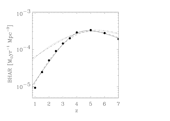
Figure 9.— Top panel: The evolution of the black hole mass density in our model. The majority of black hole mass is assembled by $z\sim 4$. Bottom panel: The evolution of the black hole accretion rate (BHAR) density in our model for black hole activity described in §4. The solid circles mark the measurements from the simulations. The solid line is an analytical fit to our results using the fitting function of equation (8) and the dashed line using the function of equation (9) where the numerator is $\propto\chi^{4}$ instead of $\chi^{2}$. The dashed-dotted and dotted lines show the fits to the cosmic star formation history in the simulation set analyzed by Springel & Hernquist (2003b) and Hernquist & Springel (2003), but scaled down by a factor of $500$. In our model, the black hole accretion rate density has a peak at similar redshifts as the star formation rate density, but it decreases faster at low redshifts.

5. The black hole accretion history

The evolution of the mass density of black holes predicted from our model is shown in the top panel of Figure 9. Extrapolating to redshift $z\sim 0$, we obtain $\rho_{\rm BH}\sim 2-4\times 10^{5}\hbox{$\rm\thinspace M_{\odot}$}{\rm\thinspace Mpc}^{-3}$, which is within $20-30\%$ of the value obtained by Merritt & Ferrarese (2001), and is roughly consistent with the result of $\rho_{\rm BH}=(2.5\pm 0.4)\times 10^{5}\hbox{$\rm\thinspace M_{\odot}$}{\rm\thinspace Mpc}^{-3}$ derived by Yu & Tremaine (2002) using the velocity dispersions of galaxies in the SDSS (also similar to the value of Salucci et al. 1999). Values inferred from the X-ray background lie typically somewhat higher, in the range of $\rho_{\rm BH}=6-16.8\times 10^{5}\hbox{$\rm\thinspace M_{\odot}$}{\rm\thinspace Mpc}^{-3}$ (Fabian & Iwasawa 1999; Elvis, Risaliti & Zamorani 2002). Although the most recent X-ray constraint from Chandra observations give $\rho_{\rm BH}\sim 2-4\hbox{$\rm\thinspace M_{\odot}$}{\rm\thinspace Mpc}^{-3}$ (Cowie et al. 2003). Note that Figure 9 clearly shows that the majority of the black hole mass is already built up by $z\sim 4$.

In the bottom panel of Figure 9, we plot the evolution of the comoving black hole mass accretion rate density according to our model. As suggested by the cumulative black hole mass function in the top panel, the peak of the black hole accretion rate per unit volume occurs at redshifts around 4-5.

It is also interesting to compare the black hole accretion rate density (BHAR) directly with the cosmic star formation rate density (SFR), as measured by Springel & Hernquist (2003b) for the simulation set we analyze here. The dashed line in the bottom panel of Figure 9 shows an empirical double-exponential fit used by Springel & Hernquist (2003b) to approximately describe the simulation results for star formation, here rescaled by a factor $2\times 10^{-3}$.

Comparing this fit with our results for black hole growth, it is evident that the shapes of the BHAR and SFR histories are quite similar in general, particularly at high redshifts, but that the BHAR history more steeply declines at low redshifts.

We may hence also try to use the double exponential function employed by Springel & Hernquist (2003b) to fit the BHAR. Using the ansatz

$$\dot{\rho}(z)=\epsilon\frac{b\exp[a(z-z_{m})]}{b-a+a\exp[b(z-z_{m})]},$$ (11)

we obtain a good fit for our measurements of the BHAR with parameter values $a=5/4$, $b=3/2$, $z_{m}=4.8$ and $\epsilon=\epsilon_{\rm BH}=3\times 10^{-4}\hbox{$\hbox{$\rm\thinspace M_{\odot}$}{\rm\thinspace yr}^{-1}\,$}{\rm\thinspace Mpc}^{-3}$. This fit is shown as the solid line in the bottom panel of Figure 9.

Compared to the SFR history, the peak of the BHAR appears to occur at slightly lower redshift, but the high-z evolution is nevertheless broadly similar, suggesting that the evolution of both rates is largely driven by the rapid gravitational growth of the halo mass function in this regime. Note however that even at its peak, the black hole accretion rate density is roughly a factor 500 lower than the star formation density, implying that the rate at which baryons are locked up in stars always far exceeds that in black holes.

It is also interesting to compare our results and the differences between the SFR and BHAR in terms of the analytic model given by Hernquist & Springel (2003) for the cosmic star formation history. Using detailed analytical arguments based on the dependence of the SFR on cosmological growth of structure and the physics of star formation, they derived a fitting function for the SFR history given by

$$\dot{\rho}_{\ast}(z)=\dot{\rho}_{\ast}(0)\frac{\chi^{2}}{1+\alpha(\chi-1)^{3}\exp(\beta\chi^{7/4})},$$ (12)

where $\chi\equiv[H(z)/H_{0}]^{2/3}$, and where $\alpha$, $\beta$ and $\dot{\rho}(0)$ are parameters. In fact, Hernquist & Springel (2003) showed that this form (also drawn as the dotted line in Fig. 9) provides a more accurate fit to the simulation results for the star formation rate than equation (11).

In particular, Hernquist & Springel (2003) demonstrated that the low redshift dependence of the star formation rate, $\dot{\rho}_{\ast}(z)\propto H(z)^{4/3}$, is primarily caused by the declining efficiency of gas cooling, which itself is related to the expansion rate of the universe, as measured by the evolution of the Hubble constant, $H(z)$. At high redshifts on the other hand, the evolution is driven by the gravitational growth of structure. It is therefore not too surprising that the BHAR closely matches the SFR at high redshifts, but shows a different behavior at low redshifts, since we assumed that black hole accretion is not linked in the same way as star formation to gas cooling, but instead to stellar feedback processes, most notably to galactic outflows. In the bottom panel of Figure 9 we also show a fit to the BHAR using a function similar to equation (12) where, in order to fit the steeper decline at intermediate to low redshifts we have assigned the numerator to be $\propto\chi^{4}$ instead of $\propto\chi^{2}$ (and $\alpha=0.013$, $\beta=0.12$ and $\rho_{\rm BH}(0)=2.2\times 10^{-4}\dot{\rho}_{\ast}(0)$). At intermediate to low redshift the BHAR therefore scales as $\dot{\rho}_{BH}\propto\dot{\rho}_{\ast}(z)\times H(z)^{4/3}\propto H(z)^{8/3}$; i.e. roughly as the square of the cooling rate. This new scaling may arise as a result of the fact that gas is depleted by the joint effects of star formation and feedback. The BHAR then may scale in proportion to both the star formation (which scales as $H(z)^{4/3}$ in this regime) and the feedback processes (which themselves scale as the SFR), hence as the square of the cooling rate. In future work, we will investigate in more detail possible physical processes underlying this scaling by means of analytical arguments.

6. Conclusions

We have explored the hypothesis that black hole growth and activity at the centers of galaxies is primarily regulated by the evolution of the total baryonic gas mass content of galaxies. We have used $\Lambda$CDM cosmological hydrodynamic simulations, which include a converged prescription for star formation, to follow the evolution of the baryonic mass in galactic potential wells. Using the numerical models, we have searched for correlations in the large-scale properties of galaxies that match those of the observed black holes. Note that with such an approach, resolving the properties of the actual small-scale accretion flows around black holes is not important.

We have shown that the steep power law form of the observed $M_{\rm BH}-\sigma$ correlation can be understood over an interesting regime of circular velocities and redshifts if there is a simple linear relation between the total gas mass (subject to star formation and associated feedback) in galaxies and their black hole mass. We find that the observed black hole mass density is consistent with $M_{\rm BH}\sim 0.004h^{-1}M_{\rm gas}$; i.e. the central black holes contain $\mathrel{\hbox to0.0pt{\lower 3.0pt\hbox{$\sim$}\hss}\raise 2.0pt\hbox{$<$}}1\%$ of baryons in galaxies. The total amount of gas in galaxies, and hence their black hole mass, may saturate simply in response to star formation, and in particular to supernova feedback and galactic winds. By considering these as the only physical processes regulating the growth of black holes, we predict that the steep dependence of black hole mass on velocity dispersion is tight but not set in primordial structures, but only fully established at low redshifts, $z\mathrel{\hbox to0.0pt{\lower 3.0pt\hbox{$\sim$}\hss}\raise 2.0pt\hbox{$<$}}2$. Once the relationship is established, we find that the black hole mass is related to the dark matter mass by $M_{\rm BH}/{10^{8}\hbox{$\rm\thinspace M_{\odot}$}}\sim 0.7(M_{\rm DM}/10^{12}\hbox{$\rm\thinspace M_{\odot}$})^{4/3}$.

We assume that all galaxies undergo a quasar phase with a typical lifetime, $t_{Q}\sim$ a few $\times 10^{7}$ yr (of the order of the Salpeter time) and show that the evolution of the quasar gas supply (taken as the $\sim 1\%$ fraction of the total gas) in spheroids is sufficient to explain, for the most part, the decrease of the bright quasar population at redshift $z<3$. However, at redshift $z\sim 1$ the predicted shape of the luminosity function differs from observations implying that mass dependent variations in the typical accretion timescale or radiative efficiency are likely to be important. An additional possibility is that there is significant intrinsic obscuration (as suggested by recent Chandra constraints on the hard XRB; e.g., Rosati et al. 2002) which may also be mass dependent.

The quasar number density at high redshift in our model does decline, but under the simplest assumption of a redshift independent $t_{q}$, it can still exceed the SDSS space density of bright quasars at $4\mathrel{\hbox to0.0pt{\lower 3.0pt\hbox{$\sim$}\hss}\raise 2.0pt\hbox{$<$}}z\mathrel{\hbox to0.0pt{\lower 3.0pt\hbox{$\sim$}\hss}\raise 2.0pt\hbox{$<$}}6$ (e.g., Fan et al. 2001a,b) by a factor $\sim 2$ or more. However the observed $B$-band number densities at $z\mathrel{\hbox to0.0pt{\lower 3.0pt\hbox{$\sim$}\hss}\raise 2.0pt\hbox{$>$}}4$ may be significantly biased low by dust along the line of sight (Pei 1995; Fan et al. 2001a), as is suggested by observations of high redshift quasars which are found to reside in dusty environments (e.g., Omont et al. 1996; Carilli et al. 2000, 2001). These biases in in B-band selection can be circumvented by a comparison of our predictions with the newly constrained comoving number density of X-ray selected quasars (Cowie et al. 2003). We have done this and find that the model yields the observed evolution of number density of X-ray faint quasars over the whole redshift range $1<z<6$ although the statistical significance of these observations is still not very high.

We further note that any freedom we have to change the luminosity function of quasars in our model comes down to our ability to select the accretion timescale $t_{Q}$, which is our only free parameter in the model. This is a fundamental parameter which governs black hole and quasar evolution, and observational constraints on its value will make our model predictions more firm and comparisons with data even more interesting. In the next few years constraints on quasar lifetimes are likely to become available from study of the clustering and the proximity effects of quasars mostly from the SDSS.

It has been shown that models based on the Press-Schechter formalism, where the quasar luminosity function is related to the dark matter halo mass, and quasar emission is assumed to be triggered by galaxy mergers, can reproduce the statistical properties of the observed SDSS quasar luminosity functions if appropriate assumptions for the quasar duty cycles are made (e.g., Wyithe & Loeb 2002; Volonteri et al. 2002; Hatziminaoglou et al. 2002). However, in these models, the decrease in merging rates is not sufficient to reproduce the luminosity functions at low redshifts and additional modeling of the evolution of the gas fraction is then required (Kauffmann & Haehnelt 2000). This highlights the importance of properly including the physical processes that govern the evolution of baryons trapped in halos as well as the growth of galaxies and their interactions. In this work we did not assume that quasar emission is triggered by galaxy mergers, but simply assumed that all galaxies that are star-forming have an equal probability of hosting a quasar. Because the quasar lifetime $t_{Q}$ is short, there can be many generations of quasars in our model, but the number density of quasar hosts is significantly larger at high redshifts, where $t_{Q}$ becomes a more significant fraction of the age of the universe than at low redshifts.

We have used our model for the relation between gas mass and black hole mass to predict the evolution of the black hole mass density in galaxy centers. We have shown that if black hole mass is assembled by gas accretion, our predicted value for the black hole mass density $\rho_{\rm BH}\sim 2-4\times 10^{5}\hbox{$\rm\thinspace M_{\odot}$}{\rm\thinspace Mpc}^{-3}$ (extrapolated to $z=0$) is consistent with observational estimates for the local value (Yu & Tremaine 2002). We find that the large majority of black hole mass is assembled up to and preceding the peak of the bright quasar phase at $z\sim 3$ and that almost no further growth takes place at lower redshifts.

We have also derived the evolution of the black hole accretion rate density (BHAR) and showed that the majority of black hole accretion should occur in the high density environments at $z\sim 4-5$, in rough correspondence with the peak of the star formation rate (SFR) history in the simulations. This is consistent with the derived black hole mass density evolution and implies that the peak of the optically bright quasar phase occurs only when the largest black holes are already assembled. At very high redshift, the BHAR and the SFR evolve similarly, both primarily driven by the rapid gravitational growth of structure, while at low redshift, the BHAR declines much more rapidly. Although the peak of the BHAR occurs close to that of the star formation rate, its normalization is a factor of a few hundred lower than that of the cosmic SFR. It hence seems unlikely that black hole accretion plays a crucial role for the gas dynamics in galaxies, and it may even be relatively unimportant for the general process of galaxy formation, unless there is strong energetic feedback by active QSOs that affects galaxies in a significant way. In future work we will investigate the predictions of this model for very high redshifts and in particular its implication for the nature of the ionizing background.

REFERENCES

Adams F.C., Graff D.S., & Richstone D.O., 2001, ApJ, 551, L31

Baes, M., Buyle, P., Hau, G.K.T., & Dejonghe, H.., 2003, MNRAS, in press (astro-ph/0303628)

Baganoff et al., 2002, ApJ, submitted (astro-ph/0102151)

Barger, A. J. and Cowie, L. L. and Mushotzky, R. F. and Richards, E. A., 2001, AJ, 121, 662

Barger A.J., Cowie L.L., Capak P., Alexander D.M., Bauer F.E., Brandt W.N., Garmire G.P., Hornschemeier A.E., 2003, ApJ, in press (astro-ph/0301232)

Boyle B.J., Shanks T., Croom S.M., Smith R.J., Miller L., Loaring N., Heymans C., 2000, MNRAS, 317, 1014

Burkert A., & Silk J., 2001, ApJ, 554, L151

Carilli C.L. et al. 2000, ApJ, 533, L13

Carilli C.L. et al. 2001, ApJ, 555, 625

Cattaneo A., 2000, MNRAS, 324, 128

Ciotti L., van Albada T.S., 2001, ApJ, 552, L13

Cowie L.L., Barger A.J., Bautz M.W., Brandt W.N., Garmire G.P., 2003, ApJ, in press (astro-ph/0301231)

Davé, R., Hernquist, L., Katz, N., Weinberg, D.H., 1999, ApJ, 511, 521

Di Matteo T., Allen S.W., Fabian A.C., Wilson A.C., Young A.J., 2003, ApJ, 582, 133

Elvis M., Risaliti G., Zamorani G., 2002, ApJ, 565, L75

Elvis et al., 1994, ApJS, 95,1

Fabian A.C., Iwasawa K., 1999, MNRAS, 303, 34

Fall S.M., Pei, Y.C., 1993, ApJ, 402, 479

Fan et al., 2001a, ApJ, 121, 54

Fan et al., 2001b, ApJ, 122, 2833

Ferrarese L. & Merritt D., 2000, ApJ, 539, L9

Ferrarese L., 2002, ApJ, 578, 90

Gebhardt K., Rich R.M., Ho L., 2002, ApJ, in press (astro-ph/0209313)

Gebhardt K. et al., 2000, ApJ, 539, L13

Gerssen J., van der Marel R.P., Gebhardt K., Guhathakurta P., Peterson R.C., Pryor C., 2002, AJ, in press (astro-ph/0210158)

Governato F., Moore B., Cen R., Stadel J., Lake G., Quinn T., 1997, New Ast, 2, 91

Hatziminaoglou E., Mathez G., Solanes J.M., Manrique A., Salvador-Sole E., 2002, MNRAS, submitted (astro-ph/0212002)

Haehnelt M., Kauffmann G., 2000, MNRAS, 318, L35

Hartwick F.D.A., Schade D., 1990, ARA&A, 28, 437

Heckman T.M., Legnert M.D., Strickland D.K., Armus L., 2000, ApJS, 129, 493

Hernquist L., Springel V., 2003, MNRAS, submitted, (astro-ph/0209183)

Katz, N., Weinberg, D.H., Hernquist, L., 1996, ApJS, 105, 19

Kauffmann G., Haehnelt M., 2000, 311, 576 (KH)

Kormendy J., Gebhardt K., 2001, In Wheeler J.C. Martel H. eds, AIP Conf. Proc. Vol. 586, 20th Texas Symposium On Relativistic Astrophysics. Am. Inst. Phys., New York, p.363

Kormendy J., Richstone D., 1995, ARA&A, 33, 581

Magorrian et al., 1998, AJ, 104, 372

Martin C.L., 1999, ApJ, 513, 156

Martini, P. & Weinberg, D. H. 2001, ApJ, 547, 12

Merritt D., Ferrarese, L., 2001, MNRAS, 320, L30

Miyaji, T., Hasinger G., Schmidt, M., 2000, A&A, 353, 25

Mo H.J. & White S.D.M., 2002, MNRAS, 336, 112

Narayan R., 2002, in ”Lighthouses of the Universe” eds. M. Gilfanov, R. Sunyaev et al., Springer-Verlag; Garching, 2001

Omont A., McMahon R.G., Cox P., Kreysa E., Bergeron J., Pajot F., & Storrie-Lombardi L.J., 1996, A&A, 315, 1

Pei Y.C., 1995, 438, 623

Richstone D. et al., 1998, Nature, 395, 14

Rosati P. et al., 2002, ApJ, 566, 667

Salucci P., Szuszkiewicz D.P., Monaco P., Danese L., 1999, MNRAS, 307, 637

Schmidt M., Schneider D.P., & Gunn, J.E., 1995, AJ, 110, 68, (SSG)

Silk J., Rees M.J., 1998, A&A, 331, L1

Soltan, A., 1982, MNRAS, 200, 115

Sokasian, A., Abel, T., & Hernquist, L. 2003, MNRAS, 340, 473

Sokasian, A., Abel, T., & Hernquist, L. 2002, MNRAS, 332, 601

Springel V., Hernquist L., 2002, MNRAS, 333, 649

Springel V., Hernquist L., 2003a, MNRAS, 339, 289

Springel V., Hernquist L., 2003b, MNRAS, 339, 312

Springel V., Yoshida, N., White, S.D.M., 2001, NewA, 6, 79

Steidel, C. C. and Hunt, M. P. and Shapley, A. E. and Adelberger, K. L. and Pettini, M. and Dickinson, M. and Giavalisco, M.,2002, ApJ, 576, 653

Tremaine S. et al. 2002, ApJ, in press (astro-ph/0203468)

Yu Q., Tremaine S., 2002, MNRAS, 335, 965

Volonteri M., Haardt F., Madau P., 2002, Ap&SS, 281, 501

Warren S.J., Hewett P., & Osmer P.S.,1994, ApJ, 421, 412 (WHO)

Wyithe J.S., Loeb A., 2002, ApJ, submitted (astro-ph/0306154)