The dwarf LSB galaxy population of the Virgo Cluster I.
The faint-end slope of the Luminosity Function.

Abstract

The widely varying dwarf galaxy counts in different environments provide a strong challenge to standard hierarchical clustering models. The luminosity function is not universal, but seems to be strongly dependent upon environment. In this paper we describe an automated procedure for detecting and measuring very low surface brightness (LSB) features in deep CCD data. We apply this procedure to large area CCD survey fields of the Virgo cluster. We show that there are many more faint ($-10\geq M_{B}\geq-14$) low surface brightness galaxies than what would be predicted from extrapolation of the Virgo cluster catalogue luminosity function. Over our limited range of measurement the faint end slope of the luminosity function becomes $\alpha=-1.6$. The luminosity function is flatter in the inner regions of the cluster than it is in the outer regions. Although these galaxies contribute a small fraction of the total stellar light of the cluster, they may contribute significantly to the mass in galaxies if they have large mass-to-light ratios similar to those recently measured for Local Group dwarf galaxies.

1 Introduction

The Virgo cluster offers the best opportunity to study in detail large numbers of galaxies (also dwarf galaxies) over a small region of sky. It is the nearest (d$\sim 17$ Mpc, Tikhonov et al., 2000) cluster with several hundreds of galaxies ($\sim 1277$ members, Binggeli et al, 1984) and the largest dominant structure of the Local Supercluster. It is an irregularly shaped cluster, with a high abundance of spiral galaxies among the bright cluster members and a large population (80% of the total known galaxy number) of dwarf galaxies (Binggeli et al., 1985). Its size is approximately 10 degrees across the sky, which corresponds to $\sim 3$ Mpc. The crossing time for this cluster is $\approx 0.1H_{0}^{-1}$ (Trentham et al., 2002) so that cluster galaxies have had plenty of opportunities to interact with each other. The huge mass of the cluster ($M=1.2\times 10^{15}M_{\odot}$, Fouque, 2001) accelerates the member galaxies to very high peculiar velocities, so that it exhibits the highest blue-shift measured for any galaxy (IC3258, approaching us at 1600 km/sec). As suggested from its irregular structure, the cluster is made up of at least three subclusters dominated by the bright ellipticals M87, M86, M49 and thus it is probably not in a state of equilibrium: it’s a very complex unrelaxed system where the central part is dynamically old, while the large surrounding region is not virialized, but still infalling (Bohringer, 1995).

The first observations of the cluster date back to Mechain and Messier (late $18^{t}h$ century), who noticed a large concentration of nebulae in the northern wing of the Virgo constellation. The identification of the cluster as a self-gravitating system consisting of hundreds of galaxies followed soon after Hubble’s 1923 discovery of Cepheids in M31. The first systematic investigation of the cluster was carried out by Shapley and Ames (1932). Since then the Virgo cluster has been of primary importance for extragalactic astronomy. It has been subject to many studies at optical, radio, IR, and X-ray wavelengths aimed at addressing its galaxy population, evolution and gas content (for the most recent studies see Gavazzi et al, 2002 (optical & multi$\lambda$); Van Driel et al., 2000 (radio) Tuffs et al., 2002 (IR); Shibata et al, 2001 (X-ray)).

The most complete optical survey of the Virgo cluster was carried out by Binggeli et al. in 1984, using photographic plates and a visual detection method. Whilst the advantage of using photographic plates is the wide area of sky surveyed ($\approx 6^{\circ}$ around the center of the cluster in this case), the major disadvantage is the low sensitivity: the survey is incomplete for objects with $M_{B}\leq-14$, missing the numerous galaxies that dominate the numbers in the Local Group, for example. Binggeli et al. (1984) carried out an extensive systematic study of the cluster finally producing a catalogue of 2096 galaxies (the Virgo Cluster Catalogue, VCC). The papers produced by them contain photometry and morphology for the galaxies, analyze morphology and dynamics and study specific and general luminosity functions for the cluster (Binggeli et al.,1984, 1985, 1987; Sandage et al., 1984, 1985, 1985a).

Our main concern in this paper is with the numbers of faint Virgo dwarf galaxies that the subjective, visual detection method used by Binggeli et al. and others might have missed in less deep surveys. The observed galaxy counts are quantified by a determination of the galaxy Luminosity Function, LF, (described by a Schechter function) and particularly from the value of its faint end slope, $\alpha$. After correction for incompleteness, Binggeli et al. found a value for the faint end slope of $\alpha\sim-1.35$. Following on from the Binggeli et al. survey, Impey et al. (1988) used a photographic amplification technique to reach lower surface brightnesses. They found numerous additional LSB dwarf galaxies not included in the VCC and derived a value of $\alpha\sim-1.7$. Using the same technique they also obtained a steepening in the faint end slope of the Fornax cluster from -1.3 to -1.55 (Bothun et al., 1991).
A more recent study of the Virgo cluster by Phillipps et al., 1998 (again using photographic plates) produced a steeper slope again ($\alpha\sim-2.0$). Phillipps et al. used a statistical method to obtain the luminosity function, subtracting faint galaxy number counts of fields outside of the cluster from those containing the cluster. This technique is very delicate because two large numbers are being subtracted away from each other to leave a small residual. There are also large variations in the background counts (Valotto et al. 2001). These rather steep values for the faint end slope of the luminosity function of Virgo are consistent with some values obtained for other clusters. For example Bernstein et al. (1995) found a value of $\alpha\sim-1.4$ for the more distant Coma cluster while Kambas et al. (2000) found a very steep slope of $\alpha\sim-2.0$ for the nearby Fornax cluster.

These values differ, however, from recently determined values of the faint end slope of the field galaxy population derived from the extensive 2dF and Sloan surveys, where $\alpha\sim-1.2$ (Cross et al., 2001, Blanton et al., 2001). The field galaxy luminosity function also corresponds very well with that obtained for the Local Group, $\alpha\sim-1.1$ (Mateo, 1998).

A major concern with the measurement of the dwarf galaxy content in different environments, is the wide range of data and detection methods used by different groups and how this affects the derived value of the faint end slope. We have recently looked at fields in different environments (Sabatini et al, JENAM 2002, Roberts et al., in prep.) using data in exactly the same conditions to that described below for Virgo. Trentham et al. (2002) found that the luminosity function is strongly dependent upon environment and, as a preliminary result, we find very few dwarf galaxies in the field and around isolated galaxies, if compared with numbers in Virgo.

It is clear that an environmental dependency of the luminosity function places new and challenging constraints on current theories of galaxy formation. For example standard Cold Dark Matter (CDM) theories predict steep faint end slopes in all environments (Bullock et al., 2000). Additions to the theory, such as supernovae driven winds (Dekel and Silk, 1986) or the influence of a reheated intergalactic medium (Efstathiou, 1992) have been used to suppress dwarf galaxy formation globally. These arguments cannot be used to explain the large differences in the dwarf galaxy population content in some environments. Recently Tully et al. (2002) have suggested that dwarf galaxy numbers in different environments depend on whether the structure in which they reside is formed before or after reionization (’squelching’). They compared the Virgo cluster, which is dwarf rich, to the dwarf poor Ursa Major cluster. From their simulations they suggest that Virgo was assembled with its dwarf galaxy population before reionization and Ursa Major after, so that dwarf galaxy formation was suppressed. There is though, as they say, only ’qualitative’ agreement between the model and the observations. Moore et al. (1999) offer more of a nurture rather than a nature explanation to the problem. Their galaxy ’harassment’ model provides a mechanism for the formation of dwarf galaxies in the cluster environment through disruption of discs due to tidal interactions with the cluster and individual galaxies. The nature of the dwarf galaxy population is then very dependent on the dynamical properties of the cluster (crossing time, galaxy number density). The Virgo cluster has a very short crossing time (0.1 $H^{-1}_{o}$) compared to Ursa Major (0.5 $H^{-1}_{o}$) (Tully et al. 2002). Thus the Virgo cluster galaxies have had more opportunities to become ’harassed’. In a study of the dynamical properties of Virgo cluster galaxies Conselice et al. (2001) describe evidence supporting the idea that the dwarf galaxies are dynamically distinct from the older cluster galaxy population and have thus been derived from an infalling population as envisaged by the Moore et al. harassment model.

An accurate derivation of the dwarf galaxy population as a function of environment is the only way to distinguish between these models. We need a detailed comparison of the luminosity function derived consistently for galaxies in different environments with those predicted by CDM, squelching and harassment. This is the first of a series of papers in which we will study in more detail the dwarf galaxy population identified in Virgo and then we will derive the environmentally dependent luminosity function of galaxies for comparison with the models.

Dwarf galaxies are extremely difficult to detect because they generally have both very low luminosity and surface brightness. To detect objects like this we need an optimum filter to enhance the signal and a set of selection criteria that preferentially selects cluster members rather than background galaxies. We also require an automated and repeatable procedure that can be applied consistently to data taken from a large area survey.

The paper is organized as follows: in section 2 we present the Isaac Newton Telescope (INT) Wide Field Camera (WFC) survey data (http://www.ast.cam.ac.uk/ wfcsur/index.php). In section 3 we discuss the methods used to determine cluster membership and to assess possible background contamination. In section 4 we describe the detection algorithm (see also Sabatini et al., 1999; Scaramella et al., in prep.). The luminosity function and first results are presented in section 5.

2 Data

The data we use are part of the INT WFC survey, that is a multi-colour CCD based wide field survey covering an area of $\sim 200$ deg². The camera is mounted at the prime focus of the 2.5m INT on La Palma, Canary Island, it consists of 4 thinned EEV 2kx4k CCDs with pixel size 0.33” and has a field size of 34.2’x34.2’ (neglecting the 1’ inter-chip spacing). The data for the Virgo survey were acquired during observing runs in Spring 1999 to 2002 and consist of two perpendicular strips of B and I band CCD images extending from the center of the cluster (identified as M87) outward for 7 and 5 degrees respectively (see fig 1). The total area covered is $\sim 25$ deg² and the average sky noise corresponds to $\sim 26$ B mag/ sq arcsec. With the use of the techniques we describe in sec. 4, these deep data allow us to study the population of dwarf galaxies down to very faint limiting central surface brightnesses ($\sim 26B$ mag/sq arcsec) and absolute magnitudes ($M_{B}\sim-10$) (see below). The results presented in this paper make use of the East-West strip, that includes M87.

Figure 1: Plot of the Virgo Cluster members as from the VCC. Overlayed are the areas covered by the INT WFCS.

The data were preprocessed and fully reduced using the Wide Field Survey pipeline. This includes de-biassing, bad pixel replacement, non-linearity correction, flatfielding, defringing (for I,Z bands) and gain correction. The photometric calibration makes use of several (5-10 per night) standard stars and the zero-points are accurate to 1-2$\%$. For the details see http://ast.cam.ac.uk/ wfcsur/pipeline.html. World Coordinate System (WCS) information is embedded in the reduced images FITS header and the astrometric calibration errors are $\leq$ 1 arcsec. The median seeing was 1.9 arcsec.

3 Membership determination and background subtraction.

Membership determination is one of the crucial and controversial problems in the study of galaxy populations in nearby clusters (Valotto et al., 2001). The properties of the background galaxies need to be studied in detail in order to minimize contamination in the sample. With the aim of deriving selection criteria which will enable us to separate cluster from background galaxies, we have carried out numerical simulations of the galaxy population in order to identify distinguishing properties of member and non-member galaxies.
The final goal is to find selection criteria that minimize the background contamination in the sample and at the same time maximize the number of Virgo cluster members selected. We have then tested the validity of the derived selection criteria in two ways (see ahead):

1. by considering the fall in surface density of our detections with increasing distance from the cluster centre.

2. by measuring the number of background galaxies detected, using our selection criteria, on fields outside the cluster.

3.1 Numerical Simulations of a cone of universe

The effects of redshift on the properties of a galaxy are mainly the following:

1. surface brightness dimming due to distance (with a dependency of $(1+z)^{4}$ + K-corrections );

2. change in apparent size with distance.

As a result, in principle, an intrinsically bright distant galaxy may appear as a faint nearby low surface brightness one and could be included in the cluster members catalogue. For example a $L_{*}$ galaxy ($M_{B}=-20$, $\mu_{0}$=21.7 $B\mu$) at z=0.2 has an apparent total magnitude of 19.5 and a $\mu_{0}$ of 23 and could be mistaken for a cluster low luminosity LSB galaxy. Its scale size however would be small (of order 2 arc sec) while a cluster dwarf with the same apparent magnitude would have a surface brightness of 24.3 $B\mu$ (because of the surface brightness magnitude relation, see below) and hence a scale size of order 4 arc sec. Thus in principle cluster galaxies can be distinguished by their larger sizes and fainter surface brightnesses at a given magnitude.

In order to quantify the trend of the apparent parameters of a galaxy with redshift we have carried out some numerical simulations: we adapted a code (Esslinger-Morshidi Z., PhD Thesis, 1997) that populates a cone of universe and detects the galaxies after applying given selection criteria. The aim is to obtain an estimate of the completeness and contamination of our sample for different selection criteria. We then use the most efficient selection criteria that preferentially select Virgo cluster galaxies. The code is composed of two parts:
1) input galaxy creation;
2) detection of the galaxies.
The cone of universe is randomly uniformly populated in space using a given cosmology, a Luminosity Function and a Surface Brightness Distribution for the galaxies. The output of this first part of the code is a catalogue of objects with given proper distance, apparent magnitude, central surface brightness and scale length (all objects are assumed to have exponential profiles). In the second part of the code, the given selection criteria are applied to the catalogue and the final output is a list of the objects that satisfy the selection criteria along with their photometric properties.

In our simulations we chose $H_{0}=75$ km s^-1 Mpc^-1, a flat universe with $\Omega_{M}=0.3$ and $\Omega_{\Lambda}=0.7$ (Lahav et al., 2002), and we analyzed a cone from redshift 0.001 to 1.5 and size $10\times 10$ sq degrees .

The luminosity function we adopted for the field is the one obtained by the 2dF Galaxy Redshift Survey (Madgwick et al., 2001) with the following parameters:

• $M_{B}*=-19.79$

• $\alpha=-1.19$

• $\phi_{*}=0.00157$ h³ Mpc^-3

and the range of input magnitudes for the galaxies is: -23 to -10.

The surface brightness distribution was chosen to follow the relationship between Surface Brightness and Total Magnitude (for recent confirmation see Blanton et al., 2001). Here we use the one given in Driver, 1999:

$$\mu_{e}\sim[(0.67\pm 0.08)M_{B}-(33\pm 6)]$$ (1)

where $\mu_{e}$ is the average surface brightness within the effective radius and for an exponential profile:

$$\mu_{e}\sim\mu_{0}+1.15$$ (2)

Using the same code with the same area (but keeping a fixed redshift of z=0.0040 $\pm$ 0.0003, corresponding to the distance of the Virgo cluster, Russell et al. 2000) we generate an artificial cluster. The Luminosity function used to describe it is normalized to the one in Sandage et al. ’85 in their survey of the Virgo cluster:

• $M_{*}=-21.4$ B mag

• $\phi_{*}=2.36$ Mpc^-3

We leave the slope $\alpha$ as a free parameter, with the purpose of running simulations with different values ($\alpha=-1.0,-1.2,-1.4,-1.6,-1.8,-2.0$). The surface brightness distribution chosen to describe the Virgo cluster is the Surface Brightness Magnitude relationship as derived by Impey et al. (1988) for Virgo:

$$\mu_{0}=0.67M+32\pm 2$$ (3)

The output catalogues produced by the code allow us to study the behaviour of apparent central surface brightness, scale length and total magnitude for simulations of the two different environments. We can then estimate what is the percentage of Virgo members and background galaxies for each bin of scale length $h$ and central surface brightness $\mu_{0}$. In fig. 2 we show how the percentage contamination by background galaxies depends on the scale length and central surface brightness of the galaxy, for the simulation with $\alpha=-1.4$ for the Virgo LF . Fig. 3 shows the histogram of scale lengths for all simulated galaxies. The dashed dotted line refers to cluster members and the filled line to background galaxies. Both figures clearly show that the best discriminating property to distinguish cluster galaxies from background ones is the scale length: as a general trend the background galaxies appear to have mainly smaller sizes and this makes it possible to separate them from Virgo members (as discussed earlier). Selecting galaxies with scale lengths $h\geq 3$ arcsec ensures that we maximize the detection of cluster galaxies compared to background galaxies (from fig. 2 contamination within this selection criteria is kept under 50 %). Being primarily interested in the low surface brightness population of the cluster we then restrict the selection to galaxies with $\mu_{0}\geq 23$.

Simulations with LF faint end slopes for the cluster steeper than that of the background give a better discrimination between cluster and background galaxies as the cluster slope increases. This is illustrated in tables 3,3,3.

Figure 2: Plot of background contamination as a function of $\mu_{0}$ (mag/sq arcsec) and h (arcsec). The numbers refer to the simulation where the LF has a faint end slope of -1.4 for the Virgo Cluster.

Figure 3: Histogram of Scale Length for both simulations: the dashed dotted line refers to Virgo members and the filled line to background galaxies.

Slope of Virgo LF = -1.0

Scale Length cut-off	Completeness	Contamination
2	93%	62%
3	83%	31%
4	72%	15%

Table 1: Completeness and contaminations for different choices of the minimum scale length selected.

Slope of Virgo LF = -1.4

Scale Length cut-off	Completeness	Contamination
2	88%	6%
3	70%	2%
4	55%	0.8%

Table 2: Completeness and contaminations for different choices of the minimum scale length selected.

Slope of Virgo LF = -2.0

Scale Length cut-off	Completeness	Contamination
2	82%	0.02%
3	60%	0.00%
4	44%	0.00%

Table 3: Completeness and contaminations for different choices of the minimum scale length selected.

In summary our simulations have shown that in order to maximize the ratio of Virgo members to background galaxies we should use a selection criteria of $\mu_{o}\geq 23$ and a scale length $h$ $\geq$ 3 arcsec. On a practical note we found that typically the seeing on our frames was a poor 2 arc sec. Convolving a 3 arc sec scale size galaxy with this seeing leads to a measured scale size closer to 4 arc sec. Thus in practice we selected objects with measured scale sizes greater than 3 arc sec which, because of the template sizes used in the method described below, means a minimum scale size of 4 arc sec.

3.2 Offset fields

As a further check to validate our selection criteria, we have applied our algorithm (see sec. 4) to another set of INT WFC data using the same detector, exposure time and filter and covering a region of sky at about the same Galactic latitude. The data we used are part of the Millennium Galaxy Survey that is a 36 arcmin wide strip going from $9^{h}58^{m}28^{s}$ to $14^{h}46^{m}45^{s}$, J2000 (Liske et al., 2002). From these data we chose a number of random fields to compare our predicted number of background detections with that of the model. The number of galaxies detected by our algorithm is 4 galaxies per sq deg. This number is in agreement both with what our numerical simulations predicted ($\sim 6$ gal per sq deg) and from what we measure for the background counts to be in the Virgo fields. It is much less than the actual number of galaxies ( $\approx 20$ gal/ sq deg) found in the Virgo cluster fields. All these points are discussed further below.

4 The detection algorithm

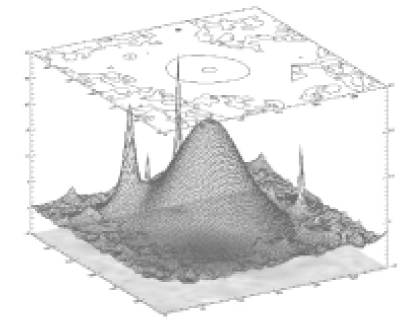
Figure 4: At the top we show the output of SExtractor for an image with a LSB galaxy from our catalogue in the centre: as can be seen, the program classifies galaxy is identified as a group of small objects rather than as an object as a whole. The detection in this case is difficoult because of the poor pixel-to-pixel signal to noise ratio for this object. As a comparison at the bottom we show the 3D output image from our algorithm for the same field. In this image the galaxy appears to be far above the noise level and thus easily detectable as a single object.

Looking for objects with a surface flux close to the sky noise requires the use of image enhancement techniques in order to optimize their detection. Standard detection algorithms for connected pixels in fact often fail on these kind of objects because of their poor pixel-to-pixel signal to noise ratio (S/N). The algorithm we have developed uses frequency domain techniques and mainly consists of convolutions of the image with matched filters: the advantage in this case is the use of the total flux of the galaxy to detect it, instead of the very low S/N pixels at its edge. As an example of this, in fig. 4 we show the finding chart produced by SExtractor (Bertin & Arnouts, 1996) for one of our fields: a LSB galaxy from our catalogue ($\mu_{0}=25.3$ mag/sq arcsec, $h$ =9 arcsec) is at the centre of the image. As a comparison we also show the output of our detection algorithm on the same image: where SExtractor finds many distinct objects at the position of the LSB galaxies, our procedure clearly distinguishes it as one.

The algorithm we used is a modified version of the method described in Sabatini et al. (1999) (for more details see Scaramella et al., in preparation) and it is composed of the following steps:

1. background fluctuation flattening

2. removal of standard astronomical objects (like stars, bright galaxies, cosmic rays etc.)

3. image convolution with matched filters that are optimized to enhance faint fuzzy structures

4. candidate classification.

LSB and dwarf galaxy candidate identification is performed on the final convolved image by means of selecting all peaks that are significantly (see sec. 4.3) above the residual noise fluctuations. The whole procedure (that includes masking, filtering, detection and measurement) is automated and its efficiency has been tested using artificial galaxies added to real images (see sec. 4.5).

Techniques involving convolution with matched filters have been used before (see for example Armandroff et al. 1998 or Flint et al. 2001) but the innovations of our method are mainly:
1) a generalization of the use of the convolution: we make use of a set of filters with several different sizes and we then combine all the convolved images in just one final significance image where objects of different scale lengths are emphasized at the same time (see par 4.3).
2) an optimization of the detection and photometry operations, that are performed at the same step using the final significance image (see par 4.4 and 4.5 for more details).

4.1 Preliminary processing

A very important issue when optimizing the detection of LSB galaxies is ensuring that the sky is as flat as possible across the image. Although the INT WFCS pipeline provides flat fielded images, we use an automatic tool from the package Sextractor in order to remove possible residual background fluctuations. The technique consists of creating a map of the background sky by interpolation of the mean values of pixels in a grid of the original image. The grid size is chosen such as to preserve the biggest scale length we want to detect with our convolution technique. Noise reduction gained in this way is about $6\%$, but a flatter background allows an easier and less contaminated application of filters and a subsequent improved measure of source fluxes.

4.2 Removal of stars and standard objects

Before convolving the image with the set of filters, we remove all the ’standard’ astronomical objects, such as stars, very bright galaxies, satellite tracks, hot pixels etc . This is necessary in order to minimize the contamination of the sample by spurious objects, i.e. objects that could simulate LSB galaxies when convolved with the filters.

The masking procedure is performed in two steps in which different kinds of objects are considered: a first step is aimed at the removal of big and bright objects, such as saturated stars or bright galaxies, and a second one aimed at small stars. Although Sextractor has the option of giving a cleaned output image, the removal is not always effective and many stellar halos remain. We have thus written our own code for bright or saturated objects and use the Sextractor procedure for the few small stars left over after our cleaning. Removal is performed by masking these objects with the local median sky value with added Poissonian noise. We use SExtractor just to detect all the standard objects in the image and select the ones to reject using a criterium based on dimension (isophotal area) and peak flux (surface isophotal flux weighted by peak flux), that clearly discriminates a stellar locus, a possible region of saturation and a region occupied by diffuse objects like galaxies (fig. 5).

Figure 5: Sextractor detections for one of our typical images shown in the plane (isophotal area, surface isophotal flux weighted by peak flux). It is clearly possible to discriminate the stellar locus, a region of saturation and a region occupied by diffuse objects such as galaxies

Once the different regions in the plot are recognized, it is possible to identify the objects we want to mask (fig. 5) . The stellar locus is fitted on each image so that the procedure is not affected by any change in the seeing value. Once the stellar locus is fitted we consider a line with same slope, but constant coefficient lower of $1.5\sigma_{fit}$ and mask all the objects that are above this line. The object removal is performed masking the region with the median sky value plus its Poissonian noise. The size of the mask depends on the geometrical parameters that Sextractor gives for each object (elliptical axis and Kron radius), on peak intensity and on the radius at which the star flux falls below $1\sigma_{sky}$.

Finally the removal of small stars left after this procedure, is carried out using the star-subtracted image given by SExtractor. We obtain, in this way, a ’star-cleaned’ image.

The star-masking procedure decreases the useful area for galaxy detection, so we take this into account when calculating numbers per sq deg in the cluster.

4.3 The multi-scale filter

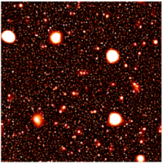
Figure 6: The top figure is a real image to which we added 3 artificial galaxies of scale length (arcsec) and central surface brightness (flux/sq arcsec) as follows: (5,1$\sigma_{sky}$),(4,2$\sigma_{sky}$), (3,3$\sigma_{sky}$). The 2 top left detections are real galaxies in the image.
Bottom figure is the final output of the algorithm it is clear that the S/N ratio is improved and they are easily detectable.

The first problem when choosing the best filter for the detection of LSB or dwarf galaxies is the determining of the optimal scale size for the filter - the sizes of these galaxies are highly variable. The necessity of selecting many different scales requires the use of either a very wide band pass filter (with the unavoidable consequence of including many different kind of objects) or the application of many different filters where we analyze the result from each one of them, requiring a huge working time. Thus we decided to build a procedure in which we apply a combination of filters of different sizes but we obtain (as described below) just one final significance image. This final image has the property of having each different size emphasized in it at the same time. We then use it as a map of candidate positions.

The filters have exponential profiles and are adjusted so that the convolution with a constant values, such as an empty area of an image, gives zero as output. Each filter is equal to zero for $r=3\alpha$ and $r=6\alpha$ (which means that it weights as positive everything inside $r=3\alpha$ (typical size of an exponential object of scale length $3\alpha$) and subtracts whatever is between $r=3\alpha$ and $r=6\alpha$). In this way we obtain a scale selective filter: everything that is smaller or bigger than the filter scale size is severely dimmed.

The cleaned image is convolved with each filter and the output is a series of convolved images. Each of them improves the signal to noise ratio (S/N) of objects with scale sizes matching the filter scale. Using these convolved images we build a final output image whose value in each pixel is equal to the maximum value assumed in the stack of convolved images . The main property of this final image is that objects corresponding to all the different sizes of filters are emphasized at the same time (fig 6).

The final image is used as a map for the positions of candidate galaxies; both detection and photometry are then performed on it. It is a significance image (as the value of each pixel is expressed in multiples of noise of the convolved image correspondent to the best matching filter) and the detection of the candidates is done taking all peaks above a $3\sigma$ threshold (see sec. 4.4). On a different array we save the filter scale on which each maximum for each pixel is found. That filter scale corresponds to the best matching scale, and this is our estimate of the scale length of the object.

From a computational point of view, once the filter scale sizes are decided, the set of filter arrays are built just once and then restored in the code at the convolution step. As a first application, we use filters with a radial symmetry, but the code also allows for the possibility of using an elliptical symmetry, which is optimized for edge on or intrinsically elongated objects.

The peak value on the output image also contains all the information we need for the photometry of the object, as shown in the following section.

4.4 Candidate classification: parameter estimation

Given the properties of the filters (see section 4.3) it can be shown that when the scale size of the filter $H$ matches the scale size of the galaxy $h$ (which is the filter scale for which the value of the convolution is found to be maximum), the value of the convolution integral is:

$$I=\int f_{0}e^{-\frac{r}{h}}(F_{*}e^{-\frac{r}{H}})2\pi rdr=\frac{F_{*}}{2}\pi f_{0}h^{2}$$
(4)

where $f_{0}e^{-\frac{r}{h}}$ is the assumed exponential profile of the galaxy and $F_{*}e^{-\frac{r}{H}}$ is just the positive part of the filter, as the object has zero flux on the negative part. Knowing the best matching scale, which corresponds to our best estimation of the object scale length, we can estimate the central original flux as:

$$f_{0}=\frac{I}{2\pi h^{2}_{\small best}F_{*}}$$
(5)

and calculate the central surface brightness.

In the ideal case of a poissonian distribution for pixels in the image and assuming pixels to be uncorrelated, we can derive a simple relationship between the noise of the original image ($\sigma_{i}$) and the noise in each convolved image ($\sigma_{o}$). Within these assumptions, for a convolution with a simple $n\times n$ box filter, the noise reduction is:

$$\sigma_{o}=\frac{\sigma_{i}}{\sqrt{n}}$$
(6)

The relation still holds for the exponential filters and in general we can then write:

$$\sigma_{o}=k(H)\sigma_{i}$$
(7)

where the coefficient k is different for each filter and is related to the filter scale size H.
Using eqs. 5 and 7 we can then show how the detection threshold on the final convolved image ($t=N_{t}\sigma_{o}$) relates to a threshold in the minimum central surface brightness which is detected for each scale length:

$$f_{0,min}=\frac{t}{2\pi h^{2}F_{*}}=\frac{N_{t}k(h)}{2\pi h^{2}F_{*}}\sigma{i}$$
(8)

However the assumption that pixels are uncorrelated is not completely true (because of PSF) and these relationships need to be calibrated for our data. In order to calibrate them we used artificial galaxies added to real images. The results of these simulations are shown in the following section.

4.5 Artificial galaxy simulations

In order to test the efficiency of the method, we ran simulations using artificial galaxies added to real images. The use of artificial galaxies allows us to test the algorithm, exploring systematically the parameter space of scale length (h) and central surface brightness ($\mu_{0}$) and thus total magnitude. The added artificial galaxies have exponential profiles (as observations indicate that this is the best representation for dwarf and LSB galaxies profiles. Davies et al., 1988), are convolved with a gaussian that simulates the seeing and are added to the real data with their poissonian noise. The use of these simulations allows us to determine the efficiency for detection and photometry of the objects.

In fig. 7 we plot the efficiency of detection as a function of scale length and central surface brightness of the artificial galaxies, where different symbols refer to different efficiencies. The efficiency is very high ($90-100\%$) over almost all of the simulated region. As expected the efficiency drops for small and faint objects because of their low S/N. We now have an estimate of completeness and contamination of our detection method and we can correct for these effects. The objects that we can detect are just the objects we want to look for in Virgo. The faintest and smallest galaxies we are able to detect correspond to $M_{B}\sim-9.5$ and the brightest and biggest to $M_{B}\sim-14.5$.

Once detected, and knowing the best matching filter scale, we can determine the central surface brightness (using eq 5) and thus the total magnitude of the objects. In figure 8 we show the difference between input values and recovered ones for the total magnitudes of the simulated galaxies. The efficiency in recovering the object’s scale length is strongly dependent on how big the gap is between the scale size of different filters. In order to obtain a good sampling of the scale lengths that we expect for dwarfs in Virgo, we decided to use the following 2,3,4,5,6,7 and 9 arcsec filter scales. Although we used smaller filters the final minimum scale size for objects in our Virgo sample is 4 arc sec (see sec. 3.1 for comments on this).

Figure 7: Detection efficiency plotted as a function of scale length $h$ and $\mu_{0}$. The CSB ($\mu_{0}$) is measured as a multiple of the sky noise and in our images this correspond to: $1\sigma\sim 26.1$mag/sq arcsec, $2\sigma\sim 25.3$mag/sq arcsec,$3\sigma\sim 24.9$mag/sq arcsec,$4\sigma\sim 24.6$mag/sq arcsec, $5\sigma\sim 24.3$mag/sq arcsec,$10\sigma\sim 23.6$mag/sq arcsec. As shown in the plot, different symbols refer to different efficiencies.

Figure 8: The measured magnitude minus input one is plotted against input total magnitude. Different symbols refer to different values of the $\mu_{0}$. The biggest errors are for very faint objects.

Although we do have some scatter in the recovered scale length and central surface brightnesses, the two compensate to give an estimation of the total magnitude with mean error of $\pm 0.5$.

The standard way of measuring photometric parameters is by fitting to the radial surface brightness profile. The detection and fitting are two distinct operations. Using our method we maximize our detection efficiency by detecting the entire image, rather than just its poor S/N edge, and we also obtain the best fitting parameters at the same time.

5 First results: The Luminosity Function

5.1 The radial number density profile of the cluster

Clusters are very interesting regions to study in order to understand the role played by the environment on galaxy formation and evolution. They are also important because it might be expected that the cluster population surface density decreases with radius from the cluster centre and eventually merges into the field. This would imply that the properties of galaxies in the outskirts of the cluster must be linked to the ones of the field population.

The sample of galaxies that we have detected with our technique extends from the centre of the cluster (identified as M87) outward for 7 degrees. Over the resulting area of $\sim 14$ sq degrees we have identified 105 new extended dwarf LSB previously uncatalogued (see VCC, Impey et al. 1988, Trentham et al. 2002).

Before discussing the implications on the luminosity function, though, we need to demonstrate that we have a Virgo cluster sample rather than a sample contaminated by background (or foreground) objects.
Background contamination has been one of our main concerns. In fig. 9 we have plotted the surface number density of our detections against cluster radius. This is the raw data: there are no corrections for contamination or completeness in this plot. As expected for a cluster member population the density decreases when going further from the centre and eventually drops to an almost constant value close to zero, approaching the cluster edge. If our sample were highly contaminated by background galaxies, we would expect an almost flat distribution of galaxies, not one dependent on distance from the centre of the cluster.

An exponential plus a constant (background) fit to the distribution gives a scale length of $2.2^{\circ}\pm 0.2^{\circ}$ (at the distance of the Virgo Cluster this corresponds to 0.7 Mpc) and a background galaxy density of $5\pm 1$ gal per sq deg. This is consistent within the errors with the value of 4 gal/sq deg found for the background in the offset fields described in section 3.2 and can thus be considered as the non-members contamination in our sample. In summary, although there might still be some contamination by background galaxies, we demonstrated it is minimal (see our numerical simulations, the offset fields number counts and fig 9)

This radial distribution can be compared with that of the bright galaxies. We have defined a Dwarf-to-Giant Ratio (DGR) which we will use in subsequent papers for comparison with different environments. This is the ratio of dwarf galaxies, definided as those with $-14\leq M_{B}\leq-10$, to giant galaxies with $M_{B}\leq-19$. We use this quantity because in some environments there are too few galaxies to construct a luminosity function.
In fig 10 we show this ratio as a function of distance from M87. Interestingly this ratio remains rather flat with a median value of $\sim 20$: the dwarfs number and giants one decline with clustercentric distance with the same scale length, resulting in a constant DGR.
Sabatini S., Roberts S. and Davies J. (JENAM, 2002) have shown evidence that the DGR is about 4 for the field population. This is just about the number you would obtain with our selection criteria if observing the Milky Way from the distance of the Virgo cluster. Out of the group of galaxies that Mateo (1998) assigns to the Milky Way just the dwarfs Sextans Fornax and Sagittarius would meet our selection criteria. Again this would give a value for the DGR of 3, lower than in Virgo. As most dwarf galaxies in clusters are probably not bound to individual giant galaxies we can also do the same test for all the dwarfs in the Local Group, in order to compare it with the Virgo Cluster. Again we obtain a DGR of 4.
Also, interestingly, the Virgo cluster DGR does not appear to smoothly blend into the field; if it did we would expect DGR to gradually decrease to the value in the field. Note also that we must be close to the ’edge’ of the cluster because the galaxy counts are about the same as those in our offset fields. Thus the Virgo cluster environment seems to be very different to that of the field even in its most outer regions.

Figure 9: In this figure we plot the number density profile of the galaxies detected within our selection criteria (h$\geq 4$, $\mu_{0}\geq 23$) versus distance from the cluster centre (identified as M87). As expected for a cluster member population the density decrease when going further from the centre and eventually drops to almost zero approaching the cluster edge.

Figure 10: Dwarf to giant ratio as a function of distance from M87. Here we define dwarf the galaxies with $-14\leq M_{B}\leq-10$ and giant the ones with $M_{B}\leq-19$. The peak at $\sim 5^{o}$ is mainly due to a dip in the distribution of giant and not to an excess of dwarfs.

5.2 The faint end slope of the Luminosity Function.

In this paper we are primarily interested in the number of dwarf galaxies in the cluster. When sufficient galaxies are available this is found by fitting to the faint end of the luminosity function. Our method enables us to detect galaxies with the following range of absolute magnitudes: $M_{B}$=-10 (h${}_{min}=4^{\prime\prime}$, $\mu_{0}^{min}=26$ $B\mu$) to $M_{B}=-15$ ($\mu_{0}^{max}=23$, h${}_{max}=9$).

An important check is to compare our derived magnitudes with galaxies common to previous catalogues of the Virgo Cluster. We have 143 galaxies in our sample that are listed in Trentham et al. 2002 and we show a plot of our measured apparent magnitudes against the Trentham et al. measurements in fig 11: a linear fit to this plot results in a slope of 1.02 and a constant value of -0.22. Our magnitudes tend to be slightly brighter then Trentham’s, but the difference lies within the errors we expect in our measurements (see fig 8). Galaxies listed in Trentham et al. 2002 that are not in our sample have been checked and they are either too bright to fall within our magnitude range or they lie in masked regions of the images (in our calculations we take into account the area lost due to the removal of stars).

Figure 11: Comparison between apparent magnitudes as measured with our method (x axis) and those in Trentham et al. 2002. A linear fit to the data gives a slope of 1.02 and a constant of -0.22.

Our derived luminosity function is shown in fig. 12. We show the raw data and the corrected data. The number of objects detected in each bin of $h$ and $\mu_{0}$ has been corrected for:

1. background contamination (as obtained from our numerical simulations of a cone of the universe).

2. incompleteness (as estimated by the detection efficiency of the algorithm with artificial galaxies).

The corrections make little difference to the numbers detected in each bin. Assuming that the drop-off in numbers beyond $M_{B}=-10.5$ is due to incompleteness we have fitted the luminosity function in the magnitude range -14.5 to -10.5. This gives a value for the faint end slope of $-1.7\pm 0.2$ for the raw counts and $-1.6\pm 0.1$ for the counts corrected for incompleteness.

Figure 12: In this figure we plot the faint end of the luminosity function. Open circles are counts for the raw data, while filled points are corrected for detection efficiency and background contamination. Squares are points from the VCC luminosity function with slope $\alpha=-1.35$, renormalized for our survey area.

It is difficult to combine galaxy counts from samples selected in different ways. For example in Kambas et al. (2000) we show how the selection of three different samples of galaxies leads to a disjoint surface brightness distribution because in each case the selection criteria preferentially picks galaxies of a given surface brightness. The surface brightness distribution of this sample (fig. 13) is also peaked.

Figure 13: Histogram of Central Surface Brightness distribution for our detections.

Even so in fig. 12 we have also shown, for comparison, the number counts for the VCC . Including the VCC data and fitting the faint end slope between -16 and -10.5 we obtain a value of -1.8 for $\alpha$ . The values that we obtain are in agreement with a steepening of the LF when including in the sample the contribution from faint and LSB galaxies. The original VCC value of -1.35 (Sandage et al., 1984) had already been brought into question by Binggeli et al. (1988) who suggested a steepening to -1.7 when including a possible dwarf population that had escaped detection. The final slope we obtain is not as steep as the one obtained by Phillipps et al. (1998) using the background field subtraction method. However, in order to compare our results with Phillipps et al., we should consider our raw data counts (as they didn’t make any correction for incompleteness) that result in a slope of $-1.7\pm 0.2$. Neglecting the last point in their LF, that might be highly background contaminated (S. Phillipps, private communication), their slope is $\sim-1.9\pm 0.15$. This then is consistent with our result.

We can also calculate a separate luminosity function for the inner and outer region of the cluster (see fig. 14). Dashed-dotted line refers to the former, while the filled line to the latter. We have chosen these regions because they correspond roughly to that part of the cluster that is within the virial radius and that which is outside it. Galaxies within the virial radius should have been much more affected by interactions with other cluster galaxies than those in the dynamically unrelaxed outer regions (Bohringer, 1995). A fit to the same range of magnitudes as for the total luminosity function results in a steeper value for the faint end slope in the outer region compared with the inner ($-1.8\pm 0.2$ and $-1.4\pm 0.2$ ). A K-S test shows that the two distributions are different with a $90\%$ probability. If confirmed by a larger statistics, this result is consistent with the idea that the faintest galaxies are more abundant in the outer regions of clusters, while in the denser inner regions they have partly been accreted by larger galaxies or have dimmed or even been disrupted by tidal interactions.

Figure 14: In this figure we plot the faint end part of the luminosity function separating the cluster into an inner (distance from M87 $\leq 0.8^{\circ}$) and outer(distance from M87 $\geq 1.6^{\circ}$) region. Dashed-dotted line refers to the former, while filled line to the latter. Although the numbers give a poor statistics, a K-S test shows that the two distributions are different with a $90\%$ probability. A fit to the same range of magnitudes as for the total LF, a steeper value for the faint end slope of the LF in the outer region compared with the inner one ($-1.8\pm 0.2$ and $-1.4\pm 0.2$ )

5.3 Total Luminosity and Mass

The total light (corrected for the area of the cluster sampled compared to the VCC) due to the population of dwarf LSB galaxies of our sample is

$$L_{Dwarf}=4\times 10^{9}L_{\odot}$$ (9)

which is just $1/50$ of that due to VCC galaxies. So this population of galaxies contributes only a small fraction of the light contributed by the bright galaxies.

A surface brightness level of about 28 B mag/sq arcsec has recently been predicted for intra-cluster light from stars associated with intra-cluster planetary nebulae (Arnaboldi et al. 2002). The average integrated surface brightness from the galaxies we detected is $\mu_{tot}\approx 32$ mag/sq arcsec in the inner region of the cluster (within $0.8^{o}$ from M87). This is far too faint to have been previously detectable as a surface brightness enhancement. This, combined with the planetary nebulae data, may indicate that there are more even lower surface brightness structures to be discovered between the galaxies.

Despite the small contribution to the light, dwarf galaxies may contribute a larger fraction to the mass. Recently very large mass-to-light ratios have been found for Local Group galaxies (see for example Mateo 1998 and particularly Kleyna et al. 2002). Assuming a mass-to-light relation as in Davies et al. (2002):

$$\frac{M}{L}=10^{3.5}L^{-0.25}$$ (10)

the total mass due to the dwarf LSB population over an area of $\sim 14$ sq deg is

$$M_{Dwarf}=1.9\times 10^{11}M_{\odot}$$ (11)

Rescaled to the total area of the cluster, this is $1/10$ of the total mass from the VCC galaxies. Given that other low surface brightness material associated with intra-cluster stars exists, it is possible that there is as much mass in the low surface brightness component of the Virgo cluster as there is in the brighter galaxies.

6 Conclusions

Observations of the relative numbers of dwarf galaxies in different environments present a strong challenge to galaxy formation models that predict large numbers of dwarf galaxies in all environments. They also present a challenge to those models that predict global suppression of dwarf galaxy formation. The Virgo cluster is a very different environment from that of the Local Group and from that of the general field. It has a very large number of dwarf galaxies compared to the giant galaxy population.

In this paper we have described a new automated technique for finding low surface brightness galaxies on wide field CCD data. We have carried out simulations to ensure that our detection method and selection criteria enable us to preferentially select cluster galaxies, rather than those in the background. From the decrease in surface number density with clustercentric distance we believe that we have achieved this goal.

Over the resulting area of $\sim 14$ sq degrees that we analysed, we have identified 105 new extended dwarf LSB previously uncatalogued (see VCC, Impey et al. 1988, Trentham et al. 2002). The resulting luminosity function is considerably steeper than that inferred from an extrapolation of the data in the VCC. The cluster luminosity function appears to be steeper in the outer parts of the cluster than in the inner part, though the dwarf-to-giant ratio remains almost constant. Although these galaxies contribute only a small fraction of the luminosity of the cluster they may contribute significantly to the galactic mass of the cluster, given recently measured large mass-to-light for Local Group dSph galaxies.

References

- [1] Armandroff T.E., Davies J.E., Jacoby G.H., 1998, AJ, 116, 2287
- [2] Arnaboldi M., Aguerri A.L., Napolitano N., Gerhard O., Freeman K., et al., 2002, AJ, 123, 760A
- [3] Bernstein G.M., Nichol R.C., Tyson J.A., Ulmer M.P., Wittman D., 1995, AJ, 110, 1570B
- [4] Bertin E., Arnouts S., 1996, A&AS, 117, 393B
- [5] Binggeli B., Sandage A., Tarenghi M., 1984, AJ, 89, 64
- [6] Binggeli B., Tammann G.A., Sandage A., 1985, AJ, 94, 251
- [7] Binggeli B., Sandage A., Tammann G.A., 1988, ARAA, 26, 509
- [8] Binggeli B., Sandage A., Tammann G.A., 1985, AJ, 90, 1681B
- [9] Blanton M.R., Dalcanton J., Eisenstein D. et al., 2001, AJ, 121, 2538
- [10] Bohringer H., 1995, Annals of the New York Accademy of Science, 759, 67
- [11] Bothun G.D., Impey C.D., Malin D.F., 1991, ApJ, 376, 404
- [12] Bullock J.S., Kravtsov A.V., Weinberg D.H., 2000, ApJ, 539, 517
- [13] Conselice C.J., Gallagher J.S., Wyse R.F.G., 2001, ApJ, 559, 791
- [14] Davies J., Phillipps S., Cawson M., Disney M., Kibblewhite E., 1988, MNRAS, 232, 239D
- [15] Davies J., Linder S., Roberts S., Sabatini S., Smith R. and Evans R., 2002, MNRAS, submitted
- [16] Dekel A., Silk J., 1986, ApJ, 303, 39D
- [17] Driver S., 1999, AJ, 526L, 69D
- [18] Efstathiou G., 1992, MNRAS, 256P, 43E
- [19] Flint K., Metevier A.J., Bolte M., De Oliveira C.M., 2001, ApJSS, 134,53
- [20] Fouque P., Solanes J.M, Sanchis T., Balkowski C, 2001, A&A, 375, 770
- [21] Gavazzi G., Bonfanti C., Sanvito G. et al., astro-ph/0205074, ApJ, in press
- [22] Impey C., Bothun G., Malin D., 1988, ApJ, 330, 634
- [23] Kambas A., Davies J., Smith R., Bianchi S., Haynes J., 2000, AJ, 120, 1316
- [24] Kleyna J., Wilkinson M.I., Evans N.W., Gilmore G., Frayn C., 2002, MNRAS, 330, 792K
- [25] Lahav O. & the 2dFGRS team, 2002, the 5th RESCEU Symposium, Tokyo, Universal Academy Press
- [26] Liske J., Lemon D.J., Driver S.P. et al., astro-ph/0207555
- [27] Madgwick D., Lahav O. et al., 2001, MNRAS, 333, 133M
- [28] Mateo M.L., 1998, ARA&A, 36, 435M
- [29] Moore B., Lake G., Quinn T., Stadel J., 1999, MNRAS, 304, 465M
- [30] Morgan I., Smith R.M., Phillipps S., 1998, MNRAS,295, 99M
- [31] Morshidi-Esslinger Z., Davies J., Smith R., 1999, MNRAS, 304
- [32] Phillipps S., Parker Q., Scwhartzenberg J., Jones J.B., 1998, ApJ 493, 59L
- [33] Phillipps S., Driver S.P., Couch W.J., Smith R.M., 1998a, ApJ, 498, L119
- [34] Russell J.S., Lucey J.R., Hudson M.J., Schlegel D.J., Davies R.L., 2000, MNRAS, 313, 469S
- [35] Sabatini S., Scaramella R., Testa V., Andreon S., Longo G., Djorgovsky G., De Carvalho R.R., 1999, SAIt proceedings
- [36] Sabatini S., Roberts S., Davies J., 2002, JENAM proceedings
- [37] Sandage A., Binggeli B, 1984, AJ, 89, 919S
- [38] Sandage A., Binggeli B., Tammann G., 1985, AJ, 90, 395S
- [39] Sandage A., Binggeli B., Tammann G., 1985a, AJ, 90, 1759S
- [40] Schombert J.M., Bothun G.D., 1988, AJ, 95, 1389S
- [41] Shibata R., Matsushita K., Yamasaki N.Y. et al., 2001, ApJ, 549, 228S
- [42] Shapley H., Ames A., 1932, Annals of Harvard College Observatory, Cambridge, Mass
- [43] Smith R.J., Lucey J.R., Hudson M.J., Schlegel D.J., Roger L.D., 2000, MNRAS, 313, 469S
- [44] Tikhonov N.A., Galazutdinova O.A., Drozdovskii I.O., 2000, Ap, 43, I 4
- [45] Trentham N., Tully B., Vereijen M., 2001, MNRAS , 325, 385
- [46] Trentham N., Hodgkin S., 2002, MNRAS, 333, 423T
- [47] Trentham N., Tully R.B., 2002, MNRAS, 335, 712T
- [48] Tuffs R., Popescu C., Pierini D. et al., 2002 ApJS, 139, 37T
- [49] Tully R.B., Somerville R.S., Trentham N. et al, 2002, ApJ, 569
- [50] Valotto C.A., Moore B., Lambas D.G., 2001, ApJ, 546, 157V
- [51] Van Driel W., Ragaigne D., Boselli A. et al., 2000, A&AS, 144, 463V