Roman Fleysher Doctor of Philosophy Physics Peter Nemethy January 2003

Search for Gamma Ray Emission from Galactic Plane with Milagro.

Dedication

Acknowledgements

There are many people who have played important roles in what I have accomplished today. Perhaps the most relevant is my NYU thesis advisor Peter Nemethy who introduced me to the subject of Galactic Gamma Rays and to the Milagro experiment. I will never forget the first month in Los Alamos when Peter had introduced me to the people of the Milagro collaboration and asked some of them to walk me through the Milagro hardware. He watched that the new (to me) acronyms such as PE, VME, TOT, ADC, TDC, DAQ are translated and explained. This allowed me quickly understand the general picture of the project. Peter is also the first member of the collaboration who treated me as a colleague rather than as a student. Latter, during preparation of this manuscript, regular meetings with Peter were essential to the progress of the data analysis. I have learned a great deal from these interactions. I thank him for all of this.

I would like to thank Todd Haines who, effectively, was my advisor while I was at Los Alamos. Todd is famous in the collaboration for his phrase: ”This will not work!”. I had always considered this phrase as an attention call signal. It drew my attention to the critic that followed from his lips. I feel fortunate that I was exposed to it. This automatically broadened my view of a problem. And, as always, a decision can be made only when several choices are considered. He is a person of great physical erudition and professional concern for students. He is a big chapter in my life which I hope will stay open for many years to come.

Another member of the Milagro collaboration and also a professor at NYU is Allen Mincer. I have met Allen even before becoming a graduate student at physics department at NYU; he was a Director of Graduate Studies at that time. In my interactions with Allen I quickly understood that he is a person of great knowledge and high moral. I value his desire to get to the roots of any problem, be it physics related or not. One rarely meets people like him. I thank both Allen and the heavens for this.

I would also like to thank several senior members of the Milagro collaboration: Gaurang Yodh, Cy Hoffman, Don Coyne, David Berley Jordan Goodman and Gus Sinnis from whom I learned many things about cosmic ray physics and life in general. I would also like to mention the other members of the collaboration. I must recognize that, involuntary, my interaction with a member was often limited by the Parkinson’s law:

interaction $\sim(a-d)$

where $a$ is the age and $d$ is the average distance to the collaboration member (both expressed in appropriate units). The collaboration spans the entire United States from the East coast to the West one, but time is on our side!!

I appreciate the many post docs and graduate students who made my time spent at Los Alamos more enjoyable. These are Isabel Leonor, Diane Evans, Rob Atkins, Joe McCullough, Morgan Wascko, Kelin Wang, Richard Miller, Stefan Westerhoff, Andy Smith, Julie McEnery and Frank Samuelson.

I would also like to thank someone whom I seldom acknowledge but often rely on, my life-long collaborator, opponent and proponent, my twin-brother Zorik. I am also indebted to my parents and my grandparents for my very existence and for the development and support of my interest in physics. Thank you.

I was very honored by the presence of professors Peter Nemethy, Todd Haines, Allen Mincer, Patrick Huggins and Alberto Sirlin at the defense of my dissertation.

Roman Fleysher
New York University
September 18, 2002

Abstract

The majority of galactic gamma rays are produced by interaction of cosmic rays with matter. This results in a diffuse radiation concentrated in the galactic plane where the flux of cosmic rays and the density of material (mostly atomic, molecular and ionized hydrogen) is high. The interactions producing gamma rays include, among others, the decay of $\pi^{0}$’s produced in spallation reactions. Gamma emission from the plane has indeed been detected in the energy range up to 30 GeV by space-based detectors. Above 1 GeV, the observed intensity is notably higher than expected in simple models, possibly implying an enhancement at the TeV region as well. Observations at TeV energies, for which the flux is too low for satellite detection, can be done with ground based telescopes. Milagro is a large aperture water Cherenkov detector for extensive air showers, collecting data from a solid angle of more than two steradians in the overhead sky at energies near 1 TeV. A 2000-2001 data set from Milagro has been used to search for the emission of diffuse gamma rays from the galactic disk. An excess has been observed from the region of the Milagro inner Galaxy defined by $l\in(20^{\circ},100^{\circ})$ and $|b|<5^{\circ}$ with the significance $2.3\cdot 10^{-4}$. The emission from the region of the Milagro outer Galaxy defined by $l\in(140^{\circ},220^{\circ})$ and $|b|<5^{\circ}$ is not inconsistent with being that of background only. Under the assumption that EGRET measurements in 10-30 GeV range can be extended to TeV region with a simple power law energy spectrum, the integral gamma ray flux with energies above 1 TeV for the region of inner Galaxy is measured to be $F(>1TeV)=(9.5\pm 2.0)\cdot 10^{-10}\;cm^{-1}\;sr^{-1}\;s^{-1}$ with spectral index $\alpha_{\gamma}=2.59\pm 0.07$. The 99.9% upper limit for the diffuse emission in the region of outer Galaxy is set at $F(>1TeV)<4.5\cdot 10^{-10}\;cm^{-1}\;sr^{-1}\;s^{-1}$ using a differential spectral index of $\alpha_{\gamma}=2.49$. The upper limit for the outer Galaxy is consistent with the extrapolation of EGRET measurements between 1 and 30 GeV. Extrapolation of the EGRET measurements between 1 and 30 GeV for the region of inner Galaxy using constant power law spectral index is incompatible with the Milagro data. This indicates softening of the spectrum at energy between 10 GeV and 1 TeV. These observations may be used to constrain some models of Galactic gamma ray emission.

Chapter 0 Introduction

Most cosmic rays are accelerated by unknown objects in our Galaxy and are trapped (for about 100 million years) by Galactic magnetic fields. The interaction of high energy cosmic rays with the interstellar material produces $\gamma$-rays by a combination of electron bremsstrahlung, inverse Compton and nucleon-nucleon processes. The nucleon-nucleon interactions give rise to $\pi^{0}$’s which decay to gamma rays and are expected to dominate the flux at energies above several GeV. In this manner, the regions of enhanced density (clouds of mostly atomic and molecular hydrogen) act as passive targets, converting some fraction of impinging cosmic rays into gamma rays. This should appear as a diffuse glow concentrated in the narrow band along the Galactic equator. Indeed, such an emission was detected by the space-borne detectors SAS 2 [6], COS B [5] and EGRET [7] at energies up to 30 GeV. Figure 1 presents the EGRET all sky survey plotted in Galactic coordinates. The Galactic plane is clearly visible.

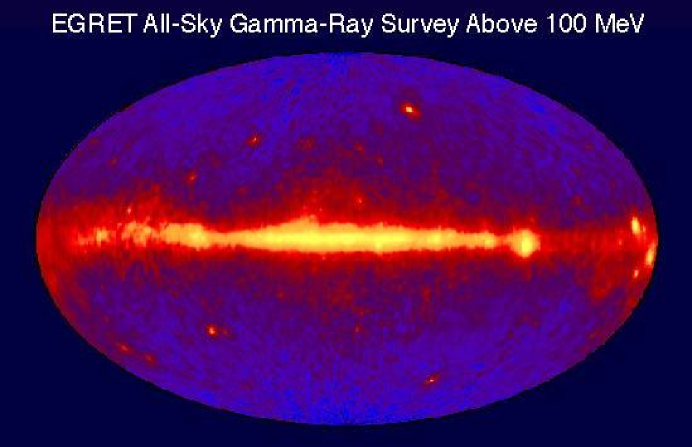
Figure 1: All sky gamma ray survey presented in Galactic coordinates. The Galactic center is in the middle of the map [10].

However, observations with present satellite based instruments at higher energies are not possible due to the rapidly decreasing flux of $\gamma$-rays, requiring bigger effective area of the detectors. Therefore, the use of ground-based arrays is needed to observe the diffuse Galactic radiation. Inasmuch as the Galactic cosmic ray spectrum extends beyond $10^{15}$ eV, the diffuse Galactic emission should extend well beyond the energy threshold of Milagro ($\sim 400$ GeV). A number of authors have estimated the expected diffuse very high energy gamma-ray flux from the Galactic plane (see for example [4]): they generally predict a flux within $\pm 5^{\circ}$ of the Galactic equator in latitude that is $\sim 10^{-4}-10^{-5}$ of the cosmic ray flux for the regions of the outer galaxy. The shape of the gamma-ray spectrum is predicted by the same authors to have power law form $\frac{dN}{dE}\sim E^{-\alpha}$, with spectral index $\alpha=2.7$. However, at TeV energies the contribution from source cosmic rays, considered by [2], may increase the expected diffuse $\gamma$-ray flux by almost an order of magnitude compared to $\pi^{0}$-decay model predictions. It is also possible that the spectrum of cosmic rays in the interstellar medium is substantially harder compared with the local one measured directly in the solar neighborhood [1] which will lead to higher diffuse $\gamma$-ray flux as well.

At present, gamma rays from the galactic plane have not been detected above EGRET energies (only upper limits were set). The only measurements that approach the required sensitivity are above 180 TeV, performed by the CASA-MIA experiment [3]. The best measurement in the 1 TeV region, which is two orders of magnitude less sensitive, is due to Whipple [8]. The present state of theoretical predictions and experimental measurements is summarized in figure 2 [9]. Milagro, a detector designed to cover the energy gap in the few TeV region between other existing instruments, should be able to detect the diffuse very high energy Galactic emission and possibly its spatial distribution and provide an enhanced understanding of Galactic cosmic rays. The sky coverage of Milagro is illustrated in figure 3. Because Milagro is located in the northern hemisphere at a latitude of $36^{\circ}$, the Galactic center is not in its field of view. However, a considerable portion of the outer disk is visible to Milagro. For a year’s exposure, Milagro is sensitive to a gamma ray flux of about that theoretically predicted.

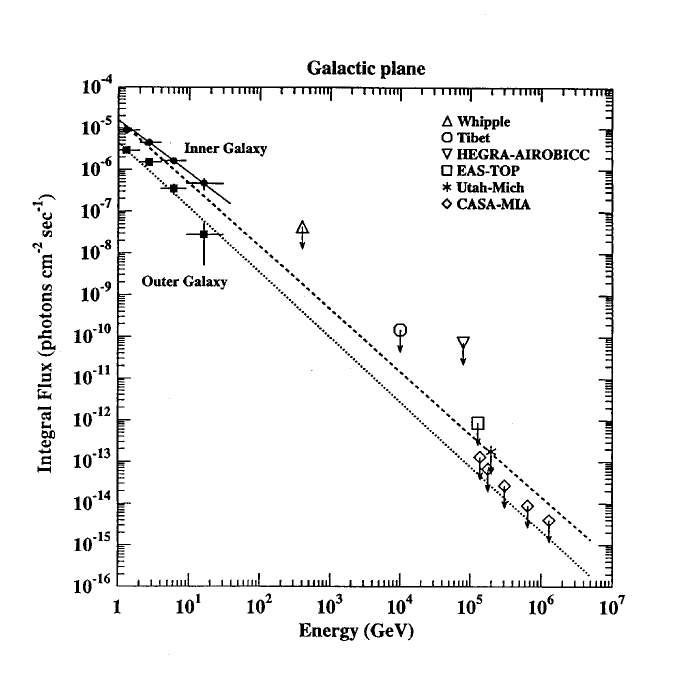
Figure 2: Theoretical predictions and observations of the diffuse $\gamma$-ray flux from the Galactic plane as a function of energy. EGRET measurements for the inner and outer regions are shown by filled points with error bars. The solid line represents the fit to the EGRET data for the inner Galaxy, indicating that the observed spectrum is significantly harder than expected (dashed line). The dotted line shows predictions for the outer Galaxy region. Identification of other instruments and their upper limits are shown as open symbols [9].

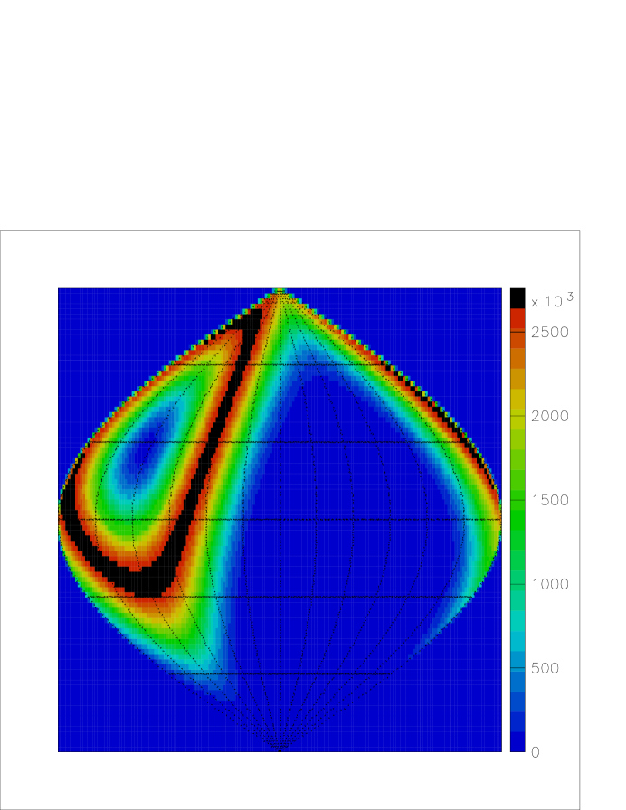
Figure 3: The density of events from Milagro (in arbitrary units) plotted in a galactic coordinate system, sine equal area projection. Grid lines are plotted every $30^{\circ}$ in longitude and latitude. The Galactic center, not visible by Milagro, is in the center of the map. Galactic longitude increases to the left.

Chapter 1 Diffuse Galactic Gamma Ray Emission.

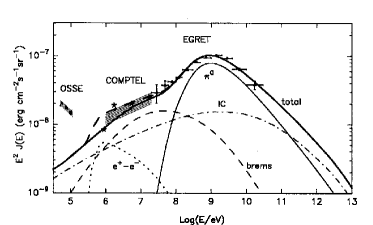
(a) The heavy solid line is the flux without contribution from positron annihilation, heavy dashed line takes it into account.

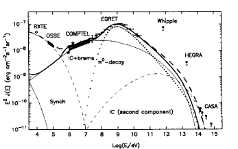
(b) The heavy solid line is the flux from the main component (figure 1(a)), heavy dashed line takes also into account a possible population of electrons accelerated to energies 250 TeV. Measurements from X-rays to very high energy gamma rays and upper limits are also shown on the plot.

Figure 1: The fluxes of diffuse radiation produced by both electronic and nucleonic components of cosmic rays in the inner Galaxy ($315^{\circ}<l<45^{\circ}$) calculated for a hard power law spectrum of electrons (with index 2.15) and protons (with index 2.1 and gradual turnover to 2.75 above few GeV). Contributions from different emission mechanisms are shown and labeled. (Adopted from [1])

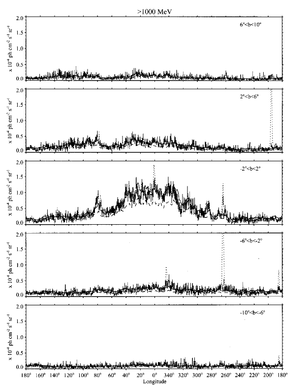
Figure 2: Longitude dependence of diffuse gamma ray emission averaged over $4^{\circ}$ wide latitude intervals in the energy range between 1 and 30 GeV measured by EGRET. The emission including point sources is shown as dotted line. The solid line is the best fit model calculated for the same energy range, convolved with the EGRET resolution function and averaged over the same latitude interval. The isotropic diffuse component added to the model for this energy range is $0.12\cdot 10^{-5}\;photons\;cm^{-2}\;s^{-1}\;sr^{-1}$. The model without the 60 % increase is shown as a dashed line. (Adopted from [7].)

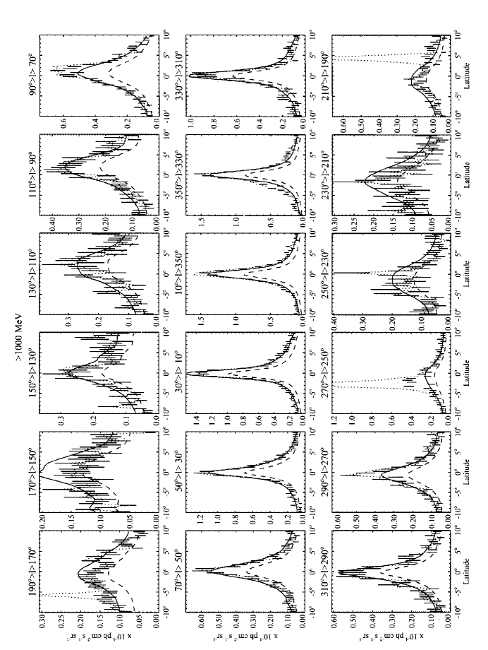
Figure 3: Latitude dependence of diffuse gamma ray emission averaged over $20^{\circ}$ wide longitude intervals in the energy range between 1 and 30 GeV measured by EGRET. See caption of figure 2 for details.

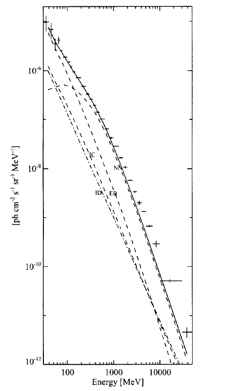
Figure 4: Average diffuse gamma ray spectrum of inner Galaxy region, $300^{\circ}<l<60^{\circ}$, $|b|<10^{\circ}$ measured by EGRET. The contribution from point sources had been removed. The model calculations plus the isotropic diffuse emission (dash-dotted line ID) is shown as solid line. The individual components of the calculation are also shown as dashed lines: nucleon-nucleaon (NN), electron bremsstrahlung (EB), inverse Compton scattering of electrons(IC) contributions. At energies above 1 GeV the data points are significantly higher than the model calculations.(Adopted from [7].)

High energy gamma rays produced by interactions of cosmic rays with the interstellar material should provide tracers of cosmic rays because their trajectories are undeflected by interstellar magnetic fields and because they traverse the Galaxy without significant attenuation. (Neutrinos would provide even better tracers because of their weak interactions.) Therefore, diffuse gamma ray emission of the Galactic disk carries unique information about the production sites, the fluxes and the spatial distribution of Galactic cosmic rays. Indeed, the separation of different emission mechanisms in a broad energy region from a few KeV to few hundred TeV in different parts of the Galaxy would provide an important insight into the problem of the origin of cosmic rays and of their propagation in the interstellar medium. This is illustrated on figure 1 [1]. Diffuse gamma radiation in the center of the Galaxy or in its halo has been proposed as a probe of annihilating dark matter particles as well [11].

The observations of the diffuse gamma ray radiation conducted in 1990’s by the EGRET detector aboard Compton Gamma Ray Observatory [7] resulted in good quality data over three decades in energy of gamma rays. The results support a Galactic origin of cosmic rays and strong correlation between the high energy gamma ray flux and the column density of the galactic hydrogen. The latter demonstrated the existence of a truly diffuse radiation based on the earlier data from SAS-2 and COS B [12].

The extraction of the diffuse component of the gamma ray emission from the EGRET data, that is the radiation produced by cosmic ray electrons, protons and nuclei interacting with the ambient gas and photon fields, is obscured by the emission from resolved and an uncertain number of unresolved point sources as well as by the diffuse isotropic emission of presumably extragalactic origin. An example of longitudinal intensity distribution of the observed emission, including the isotropic emission and excluding the point source contribution is shown on figure 2. Figure 3 shows the latitude distribution of the intensity for the same energy range. The dotted lines represent the observed emission including the point sources, the solid lines are the calculated intensities using the model described in [7, 14]. In this model, the EGRET data together with radio data was used to develop a three-dimensional picture of both gas and cosmic ray densities in the Galaxy. The diffuse gamma ray emission for energy $E_{\gamma}$ from the galactic longitude $l$ and latitude $b$, $|b|<10^{\circ}$ is given by [7, 14]:

$$j(E_{\gamma},l,b)=\frac{1}{4\pi}\int\left[c_{e}(\rho,l,b)q_{em}(E_{\gamma})+c_{n}(\rho,l,b)q_{nm}(E_{\gamma})\right]\times$$

$$\times\left[n_{HI}(\rho,l,b)+n_{HII}(\rho,l,b)+n_{H_{2}}(\rho,l,b)\right]d\rho+$$

$$+\frac{1}{4\pi}\sum_{i}\int c_{e}(\rho,l,b)q_{p}^{(i)}(E_{\gamma},\rho)u_{p}^{(i)}(\rho,l,b)d\rho$$

$$(photons\;cm^{-2}\;sr^{-1}\;GeV^{-1})$$

where $\rho$ is the distance of the line of sight in the direction of $l$ and $b$ measured from the Sun. The first integral represents the gamma ray production due to cosmic ray interactions with matter where $q_{em}(E_{\gamma})$ and $q_{nm}(E_{\gamma})$ are the electron bremsstrahlung and nucleon-nucleon production functions per target hydrogen atom based on the cosmic ray spectrum measured in the vicinity of the Sun. The functions $c_{e}(\rho,l,b)$ and $c_{n}(\rho,l,b)$ are the ratios of the cosmic ray electron and proton densities at the given location to their densities in the vicinity of the Sun. The electron and proton spectra are assumed to have the same shape as measured locally near the Sun and therefore the $c$’s are independent of energy. The ratios are also assumed to be be equal and independent of $b$: $c_{e}(\rho,l,b)=c_{n}(\rho,l,b)=c(\rho,l)$, $c(\rho=0,l)=1$. The quantities $n_{HI}(\rho,l,b)$ and $n_{H_{2}}(\rho,l,b)$ are the atomic and molecular hydrogen densities expressed as atoms per unit volume derived from the 21 cm hyperfine transition emission line (HI) and 2.6 mm kinematic $J=1\rightarrow 0$ transition line of CO surveys. The CO intensities are scaled by $2X$ where $X=N(H_{2})/W_{CO}$ is the proportionality constant between the column density of molecular hydrogen and the integrated intensity of the CO line. The distribution of ionized hydrogen $n_{HII}$ is taken from a model [7] and is shown to have small contribution to the diffuse gamma ray emission compared to that of HI and $H_{2}$. The second integral describes the contribution from inverse Compton interactions between cosmic ray electrons and interstellar photons where $q_{p}^{(i)}(E_{\gamma},\rho)$ is the inverse Compton production function based on the local electron spectrum, and the summation is over discrete wavelength bands ($i$) of cosmic blackbody radiation, infrared, optical and ultraviolet that arise from within our Galaxy with corresponding photon energy density distributions $u_{p}^{(i)}(\rho,l,b)$.

This model accurately matches the observed emission as seen by EGRET for all Galactic longitudes over the energy range from 30 MeV to about 30 GeV. The model underestimates the observations at energies above 1 GeV in the region of inner Galaxy $300^{\circ}<l<60^{\circ}$, $|b|<10^{\circ}$. (The model calculations without the 60 % increase in this region is shown as a dashed line on figures 2, 3. This is also illustrated on figure 4.) Some authors [13] have suggested that because electron propagation is limited by radiative losses the local measurements of the electron spectrum may not be representative for the entire Galaxy. In this case, a harder cosmic ray electron spectrum could be used to explain the observed excess. It is also possible [1] that the proton spectrum in the inner Galaxy is harder then observed in the Solar neighborhood, at least in the region below few GeV. Another possibility is contribution from unresolved sources. Assuming these are supernova remnants, it was shown [2] that their spatially averaged contribution to the diffuse gamma ray flux at 1 TeV should exceed the above model predictions [7] extended to 1 TeV by almost an order of magnitude. It is therefore of interest to search for the diffuse emission from the Galactic plane at energies around 1 TeV.

Chapter 2 Extensive Air Showers.

1 Longitudinal Development of Extensive Air
Showers.

The desire to detect low fluxes of gamma rays at energy around 1 TeV using ground based telescopes impels consideration of propagation of the photons to the ground level, where they can be registered.

A high energy primary gamma-ray entering the atmosphere interacts with it, initiating the production of secondary particles which in turn create tertiary particles and so on. Such electromagnetic cascades are propagated predominantly by photons and electrons. The basic high energy processes that make up the cascade are pair production and bremsstrahlung occurring in the field of nuclei of air which produce successive generations of electrons, positrons and photons. Charged particles are removed from the shower development by ionization losses, photons — by Compton scattering. The number of particles increases until their energies decrease to the critical energy $E_{c}\approx 80MeV$, when ionization and scattering become the main energy loss mechanisms. This stage of the development is called shower maximum.

Inasmuch as for ultrarelativistic particles the radiation length $X_{0}$ for the bremsstrahlung process (the amount of the material traversed over which particle’s energy is decreased by a factor of $e$, $E=E_{0}e^{-x/X_{0}}$) is approximately equal to the gamma ray interaction length for electron-positron pair production [15], it provides a convenient scale, and in the case of air it is about $X_{0}\approx 37g/cm^{2}$.

The cascade development provides an interesting example of a stochastic process which is prohibitively difficult for analytic calculations. Although several approximations have been considered [16], numerical methods are usually needed to obtain results of practical use.

Recent simulations by DiSciascio et al [17] show that the average number of photons and electrons with the energy greater than $E_{th}$ in the shower initiated by a photon with energy $E_{0}$ is well described by a modified Greisen formula:

$$N(E_{0},E_{th},t)=A(E_{th})\frac{0.31}{\sqrt{y}}e^{t_{1}(1-1.5\ln s_{1})}$$ (1)

where $t_{1}$ is the modified depth $t=x/X_{0}$ from the top of the atmosphere measured along the trajectory of the primary particle and expressed in the units of radiation length:

$$t_{1}=t+a(E_{th})$$

The parameter $s_{1}$ represents the age of the shower and increases as it develops starting at $s_{1}=0$, $s_{1}=1$ at the maximum, $s_{1}>1$ in the declining stage of the cascade:

$$s_{1}=\frac{3t_{1}}{t_{1}+2y}$$

$$y=\ln\frac{E_{0}}{E_{c}}$$

The parameterization is valid in the depth range $4<t<24$ for primary photon energies $0.1<E_{0}<10^{3}$ TeV. The coefficients $A(E_{th})$ and $a(E_{th})$ are given in the table 1. The dependence is illustrated on figure 1. The Milagro detector is situated at the vertical depth of about 20 radiation lengths, thus within the range of the simulations for photons with zenith angles between 0 and 32 degrees.

$E_{th}$,	electrons		photons
MeV	A	a	A	a
1	0.92	0.00	4.80	-0.88
5	0.75	0.19	2.98	-0.69
10	0.63	0.35	2.13	-0.57
20	0.50	0.53	1.45	-0.36

Table 1: Coefficients $A$ and $a$ for modified depth calculation [17] in longitudinal development case, equation 1.

(a) Longitudinal development of electron component.

(b) Longitudinal development of photon component.

Figure 1: Longitudinal development of gamma ray induced showers with $E_{th}=1MeV$ particle detection threshold.

2 Lateral Development of Extensive Air Showers.

As an extensive air shower cascades through the atmosphere ultrarelativistic particles and photons are produced mainly in the forward direction. However, because electrons and positrons suffer multiple Coulomb scattering off the electric fields of nuclei and photons undergo Compton scattering off atomic electrons, the particles are spread out and the shower attains a lateral distribution. The density of particles is greatest near the shower core, the trajectory that the primary gamma-ray would have had if it did not interact with the atmosphere. The average number of photons $\rho(r,t,E_{0})$ per unit area at a distance $r$ from the shower core agrees well with the Nishimura-Kamata-Greisen (NKG) formula, with modified depth parameter [17]:

$$\rho(r,t,E_{0})=\frac{N(E_{0},t)}{r_{m}^{2}}f(r/r_{m},s_{2})$$ (2)

where

$$f(r/r_{m},s_{2})=\frac{1}{2\pi}\cdot\frac{1}{B(s_{2},4.5-s_{2})}\left(\frac{r}{r_{m}}\right)^{s_{2}-2}\left(1+\frac{r}{r_{m}}\right)^{s_{2}-4.5}$$

$$t_{2}=t+b(E_{th})$$

$$s_{2}=\frac{3t_{2}}{t_{2}+2y}$$

with $B(x,y)$ being beta function so that $2\pi\int_{0}^{\infty}f(r/r_{m},s_{2})(r/r_{m})d(r/r_{m})=1$, $r_{m}$ — being Moliere scattering unit, $r_{m}=\frac{E_{s}}{E_{c}}X_{0}=9.7g\cdot cm^{-2}$ or about 110 meters at the elevation of Milagro ($E_{s}=m_{e}c^{2}\sqrt{4\pi/\alpha}\approx 21MeV$) and $N(E_{0},t)$ is total number of photons at the depth $t$ [20] given by equation 1.

It was also found in [17] that the lateral density distribution of electrons is well represented by the same expression if the scattering unit is substituted by $r_{m}^{\prime}=r_{m}/2$. (This fact that shower photons are spread farther from the shower axis than the electrons is a consequence of the fact that photons do not lose energy by ionization and can travel larger distances than electrons.) The values of parameters $b(E_{th})$ are given in the table 2.

$E_{th}$,	electrons	photons
MeV	b	b
1	0.45	0.83
5	-1.22	-1.49
10	-2.57	-3.45
20	-4.22	-5.51

Table 2: Coefficients $b$ for modified depth calculation [17] in lateral distribution case, equation 2.

The average density of photons and electrons per unit area as a function of distance from the shower core is illustrated on figure 2

(a) Lateral distribution of electron component.

(b) Lateral distribution of photon component.

Figure 2: Density of particles as a function of core distance for gamma ray induced showers with $E_{th}=1MeV$ particle detection threshold. Curves are normalized to the total number of particles in the respective components. Plots are made for showers at the depth of 20 radiation lengths.

3 Temporal Distribution of Extensive Air Shower Particles.

Once an air shower develops lateral structure, one can speak about the shower front — the forward edge of the advancing cascade. The arrival time $T$ of the earliest particle hitting a plane perpendicular to the shower axis at a distance $r$ from the core provides the information concerning the shape of the front. Since the electron component of the lateral distribution is attained due to multiple scattering, it is lower energy electrons and positrons which propagate farther away from the axis. These travel at lower speeds and one expects them to be delayed with respect to the energetic one’s at the core. The photons are expected to be more prompt than electrons, but are also delayed with respect to core due to greater distance traveled. The average arrival time of the first particle as a function of the core distance for both electron and photon components is illustrated on figure 3.

Figure 3: Average arrival time of the first particle as a function of the core distance.

It appears that the front of each of the components assumes a parabolic shape. The fluctuations of $T$ around its average appears smaller for the photon component than for electron one [17] and, in general, are quite small. The thickness of the shower is defined by the arrival time distribution of particles with respect to the front at the given distance $r$, and is, therefore, due to lower energy electrons and photons originating later in the shower cascade.

4 Cherenkov Radiation.

One of the methods of detection of high energy electrons and positrons and therefore of the air showers is with the help of Cherenkov radiation. Cherenkov radiation arises when a charged particle traverses a dielectric medium with a velocity $v$ which is greater than the speed of light in the medium $c/n$. Here $n$ is the index of refraction of the medium which, in general, depends on the wavelength of the emitted radiation and $c$ is the speed of light in vacuum. The radiation is emitted by atoms and molecules polarized by the moving particle. According to Huygens’ principle, the partial waves will interfere to create the total wavefront propagating at an angle $\theta=\arccos\frac{c}{nv}$ with respect to the velocity of the particle. At lower speeds, some energy of the particle is still lost due to polarization of the medium, however no Cherenkov radiation results.

The condition for existence of radiation $\frac{c}{nv}=\frac{1}{\beta n}<1$ can be expressed in terms of the particle’s energy:

$$E>\frac{mc^{2}}{\sqrt{1-\frac{1}{n^{2}}}}$$ (3)

where $m$ is the rest mass of the particle. For example, the index of refraction of water is $n_{water}=1.35$, and therefore the threshold energy for electron to produce Cherenkov radiation (and therefore detection threshold) is equal to 0.759 MeV. For a muon it is 0.157 GeV and for proton 1.40 GeV.

The number of Cherenkov photons produced per unit path length by such a particle with charge $Ze$ and per unit wavelength [18]:

$$\frac{d^{2}N}{dxd\lambda}=\frac{2\pi\alpha Z^{2}}{\lambda^{2}}\left(1-\frac{1}{\beta^{2}n^{2}(\lambda)}\right)$$

or, in terms of emitted energy:

$$\frac{d^{2}E}{dxd\lambda}=\frac{\pi e^{2}Z^{2}}{\epsilon_{0}\lambda^{3}}\left(1-\frac{1}{\beta^{2}n^{2}(\lambda)}\right)$$

where $\alpha=\frac{e^{2}}{4\pi\epsilon_{0}\hbar c}$ is fine structure constant. Here, we have made explicit the dependence of the index of refraction on wavelength. Cherenkov radiation is emitted preferably in the short wave region (blue/violet end of the visible spectrum).

Note that for ultrarelativistic particles $\beta\approx 1$, the Cherenkov angle in water is approximately $42^{\circ}$ and the emitted energy becomes independent of the particle’s energy. This fact can be used to provide absolute energy calibration of photodetectors.

5 Detection of Extensive Air Showers.

Air showers produced by high energy photons consist mainly of electrons, positrons and lower energy photons, and thus hint at methods of detection. If the energy of the primary photon is greater than about 10 TeV, then there are enough particles in the cascade reaching the surface of the Earth to enable the detection by arrays of scintillation counters where energy of charged particles is converted into flashes of visible light. These flashes are detected by photoelements. The detectors of this type are called extensive air shower arrays (EAS arrays). CASA-MIA and Tibet are examples of such arrays. The determination of the arrival direction and of the primary energy of air showers, sampled by a detector array, makes use of the lateral distribution function over a wide range of distances: the arrival time of the shower particles is used to determine the direction, the measurements of the particle density as a function of core distance together with the direction provide information about the energy of the primary gamma ray.

Cascades, initiated by a primary photon with energy below several hundred GeV do not reach the ground, but can be detected by Cherenkov radiation that charged particles emit in the air as the cascade develops. Such detectors are termed air Cherenkov telescopes, such as Whipple and HEGRA. Detectors of this type, being optical devices, make use of the fact that most of the Cherenkov light is emitted in the forward direction of the primary particle and rely on their angular resolution — truly a telescope type of a measurement. Arrival direction and energy of the primary particle is inferred on the basis of the imaged longitudinal development of the air shower.

Other types of detectors which were used to detect secondary particles are bubble chambers, spark and ionization chambers. Such methods are rarely used nowadays. Instead, atmospheric Cherenkov telescopes and extensive air shower particle detector arrays constitute the two major ground-based techniques.

6 Cosmic Rays. Difference Between Cosmic Ray and Gamma Ray Induced Showers.

The discussion has been concerned so far with the air showers produced by primary gamma rays. However, among the particles entering the Earth’s atmosphere gamma rays present a fraction of less than 0.1%. About 79% of the particles are high energy protons and 14% are alpha particles. The rest are nuclei of heavier atoms: carbon, nitrogen, oxygen, iron,…

Just as in the case of gamma rays, high energy hadrons also initiate air showers when they enter the atmosphere. However, the processes in a hadronic cascade are quite different from the electro-magnetic one.

In such a cascade an incident hadron undergoes strong interactions with the air nuclei in which protons, neutrons, mesons and hyperons are created in quantities determined by their relative cross-sections. The most numerous particles are that of the pion triplet.

The charged pions have a lifetime of about $2.6\cdot 10^{-8}$ seconds and, if they did not interact first, decay into muons and neutrinos:

$$\pi^{+}\rightarrow\mu^{+}+\nu_{\mu}$$

$$\pi^{-}\rightarrow\mu^{-}+\bar{\nu}_{\mu}$$

which gives rise to a muonic component of the cascade. If the energy of charged pions is high, then, due to relativistic time dilatation, they will have the opportunity to interact with a nucleus rather than decay, thus producing secondary particles which replenish the hadronic component of the cascade. Neutral pions, on the other hand, have a much smaller lifetime of about $10^{-16}$ seconds and decay, dominantly, into photons ($\pi^{0}\rightarrow\gamma+\gamma$). If energy of photons is above critical, they will initiate electromagnetic cascades. It is due to presence of the electromagnetic component the hadron induced air showers are very similar to those initiated by gamma rays. Muons, produced in the cascade, have a lifetime of $2.2\cdot 10^{-6}$ seconds and high energy ones survive to the sea level because of time dilatation.

Thus, in a hadron cascade, the secondary particles either interact again, decay or are absorbed as a result of ionization energy loss. The cascade builds up to a shower maximum as in an electromagnetic cascade after which the numbers decrease. Because decay muons do not interact by strong interactions and loose less energy in bremsstrahlung radiation then electrons, they primarily loose energy by ionization and therefore have a slower decrease. Because detection of high energy gamma rays relies on registration of secondary particles, the extensive air showers produced by cosmic rays constitute background noise for ground-based gamma-ray detectors. Special techniques and algorithms have to be developed to suppress this noise in order to increase the sensitivity to photon primaries. The presence of muons in the hadron induced shower is often exploited.

7 Milagro: a Next Generation of EAS Array.

The design of a detector has to reflect the goals and the obstacles mentioned above. The great success of air Cherenkov telescopes is due to their excellent angular resolution and good background rejection. With advantages come its limitation. Because the energy threshold for electrons to produce Cherenkov radiation in air is about 21 MeV ($n_{air}=1.000293$, formula 3), it cuts the number of detectable particles by a factor of 2 (table 1, equation 1). This bounds the energy of the primary gamma rays detectable by the technique to be greater than about 100 GeV. Furthermore, the telescopes are narrow-field-of-view optical devices, therefore, they can observe only a small portion of the sky at a time during cloudless, moonless nights. This severely impacts on their ability to detect transitory sources and perform observations of extended sources.

Extensive air shower arrays, on the other hand, can observe the entire overhead sky and can operate 24 hours a day regardless of weather conditions. However, scintillation counters typically cover only a small fraction of area compared to lateral extent of the shower, and therefore detect only a small fraction of secondary particles leading to higher energy threshold, typically above 10 TeV.

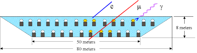
Figure 4: Schematic diagram of the Milagro detector.

Milagro achieves an energy threshold of 400 GeV by using water as a detection medium and by locating the detector at relatively high altitude. Using water allows Milagro to detect not only charged secondary particles of the air shower, but also secondary photons via Cherenkov radiation of cascades initiated by them in the water. This is important because secondary photons present a large fraction of particles reaching the ground level (table 1, figure 1). Also, the time distribution of the foremost particle appears to be narrower for the photon component than for the electron one [17] rendering the efficient conversion of secondary photons into Cherenkov radiation by the water medium even more essential.

Milagro is a covered, light tight pond filled with purified water and instrumented with photo detectors. Relativistic, charged particles produce Cherenkov radiation as they traverse the water. The radiation is emitted in a cone-like pattern with an opening angle of not greater than $42^{\circ}$. This allows Milagro to instrument a large surface area of the detector with a sparse array of photo detectors. Methods such as these have been used for decades in high energy physics [19].

As shown in figure 4, Milagro has been configured with two planes of photo detectors. The upper layer is used to measure the air shower front, providing the information needed to reconstruct the primary particle direction. The lower layer is used to detect penetrating muons or hadrons and aid in rejecting cosmic ray induced showers.

Milagro fits the classification of extensive air shower array, shares many principles but improves on detection methodology.

Chapter 3 The Milagro Detector

1 Physical Components of the Detector.

The Milagro detector is located in the Jemez mountains, about 45 km west of Los Alamos, New Mexico, at $-106^{\circ}40^{\prime}37^{\prime\prime}$ East longitude, $35^{\circ}52^{\prime}43^{\prime\prime}$ North latitude. The central detector consists of 723 photomultiplier tubes (PMT) deployed in a 60 m x 80 m x 8 m pond filled with water. The elevation of the reservoir above sea level is 2650 meters, which translates to an atmospheric overburden of 750 $g/cm^{2}$.

The buoyant photomultiplier tubes are held below the water surface by anchor cords, attached to a grid of weighted PVC pipes. The spacing of the grid is 2.8 meters. The length of each string was calculated for each PMT so that the PMTs would all lie in a horizontal plane and form a two layer structure. Each PMT is floating upright with its photocathode facing upwards. Each PMT is also surrounded by a conical baffle to block internally reflected light.

The 450 PMTs of the top layer are deployed under 1.4 meters of water and are used to measure the arrival direction of the shower. Two hundred seventy-three additional PMTs are located near the bottom of the pond under 6 meters of water and are used to distinguish photon- and hadron-induced air showers. The top layer is called the shower layer and the bottom one — the muon layer.

The complete set of PMT string attachment points was surveyed after the grid was installed.Vertical positions of the PMTs were verified after the pond was filled with water. The final accuracy of PMT coordinates is estimated to be $\pm 0.03$ m in horizontal and $\pm 0.01$ m in vertical directions. Coordinates of the PMTs are used for shower reconstruction and detector calibration. Because PMTs are used to detect Cherenkov light produced by air shower particles traversing the water, it was necessary to block the external light from entering the pond with an opaque cover and to provide for high transparency of the water. The 1 mm thick cover was made of two black layers of polypropylene with an internal polyester scrim. The cover can be inflated to allow access into the pond. High quality of the water was achieved with continuous recirculation and filtration of the water by a set of carbon filter, $1-\mu$m filter, ultraviolet lamp and $0.2-\mu$m filter. The attenuation lengths of the water in the recirculator and that of the pond are indistinguishable and equal to $13.4\pm 0.5$ meters [22].

A lightning protection system was installed around the experiment as a safeguard against possible strikes.

2 The photomultiplier tube.

The photomultiplier tube is a vacuum device used to transform very faint light signals into electric ones. It consists of a photocathode, a set of dynodes and an anode. A photon incident on the photocathode causes the emission of an electron (called photo-electron (PE)) into the vacuum tube via the photoelectric effect. This electron is directed towards the first dynode by the focusing fields. When it hits the dynode, secondary electrons are emitted, each of which is guided towards the next dynode. The dynodes are kept at different electric potentials and thus cause acceleration of electrons to sufficient energies for secondary emission to take place. As this cascade develops, the number of electrons increases exponentially and by the time it reaches the anode the number of electrons is about $10^{7}$ for every electron emitted at the photocathode.

Besides amplification, the following points motivate the choice of the Hamamatsu R5912 SEL PMT model:

• Cherenkov radiation generated by shower particles in the water is emitted mostly at the violet end of the visible spectrum. The selected model is sensitive in the 300 - 650 nm wavelength range.

• Quantum efficiency, the ratio of the number of PE produced at the cathode to the number of incident photons, is rather high: 0.2-0.25 for the selected model.

• Time resolution. Time resolution of a PMT is limited by the fluctuations in the cascade development starting from the photocathode all the way down to the anode. The variance of this transit time increases as the input intensity decreases and is 2.7 ns at the lowest input (1 PE produced).

• Late pulsing. Late pulses on the output of a PMT are believed to occur when electrons are being reflected off the first dynode and produce secondary electron only upon second re-entry into the dynode assembly caused by the focusing fields. The probability of late pulses decreases for high light intensities because the probability that all electrons produced at the cathode are reflected decreases as number of them increases.

• Pre-pulsing. Pre-pulses are considered to be caused by the light hitting the first dynode directly, thereby producing an anode signal which precedes the main one induced by the photo-electron. The Probability of pre-pulsing is higher for larger light intensities.

• After-pulsing. After pulses are thought to be caused by residual gas molecules in the tube being ionized by electrons and subsequently hitting the photocathode and producing electrons. The signal induced by these electrons follows the main anode one.

• Saturation. Saturation is the effect of decrease of the amplification coefficient of the PMT for high light intensities. This is caused by the inability of the dynodes to accelerate the increased number of the secondary electrons to sufficiently high energy.

Overall, the characteristics of the selected PMT model were found suitable for the application.

3 Electronics. Time Over Threshold.

Each PMT is connected to its own electronic channel with a single cable used to supply high voltage for the tube and to deliver a signal pulse from it. The signal carries two pieces of information about the Cherenkov light hit: the time when the hit occurred and it strength.

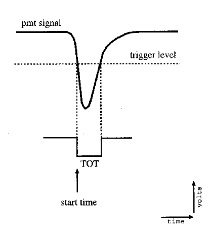
Figure 1: Time over threshold.

The time of the hit is determined by the time when the amplified signal crosses the discriminator with the preset threshold. This time is termed start time. A time-to-digital converter (TDC) is used to digitize the start time and to pass it to the data acquisition computer. Except for the saturation, the output anode charge of the PMT is proportional to the number of Cherenkov photons which struck the tube, therefore, the output charge is the measure of the hit strength.

Conventionally, analog-to-digital converters (ADC) are utilized to digitize the charge information. Because of cost, speed and dynamic range limitations of typical ADC’s, a time-over-threshold (TOT) method was adopted instead. The idea of the method is simple (figure 1). A capacitor $C$ is quickly charged by the PMT signal with total charge $Q$ and then is slowly discharged via a resistor $R$. The voltage on the capacitor as a function of time is given by:

$$V(t)=\frac{Q}{C}e^{-t/RC}$$

If the time during which the voltage exceeds the preset threshold is measured, then it is seen that

$$time\;over\;threshold\;\sim\ln Q$$

Thus, time over threshold is related to the initial charge $Q$ and provides a way to measure the signal strength. Implementation of this method allows the use of a single multi-hit TDC module to digitize both start time and the time over threshold counterparts.

In practice, two discriminators with different threshold levels (low and high) are used to guard against pre- or after-pulsing of the PMTs. These accompanying pulses are usually small and do not cross the high threshold. Therefore, the use of high threshold information is preferred where available. The low threshold was set to about 1/4 of the average signal produced by a single photoelectron and high threshold to about 7 PE.

Each shower layer PMT signal crossing the low discriminator also participated in the trigger formation process by generating a 25 mV, 300 ns long pulse [21]. The analog sum of all such pulses is sent to a discriminator with a threshold corresponding to 60 PMT being hit. If the discriminator is fired the trigger pulse is generated. Setting the trigger threshold much higher than 60 PMT would increase the energy threshold of the detector. Making it much lower would enable single muons to trigger the detector. The choice of 300 ns window is motivated by the duration of near horizontal shower propagation through the detector. The trigger provides a common stop for all TDC’s, all start times are referenced to it.

The absolute time of each triggered event is provided by a Global Positioning System clock. A schematic diagram of a PMT channel is presented in figure 2.

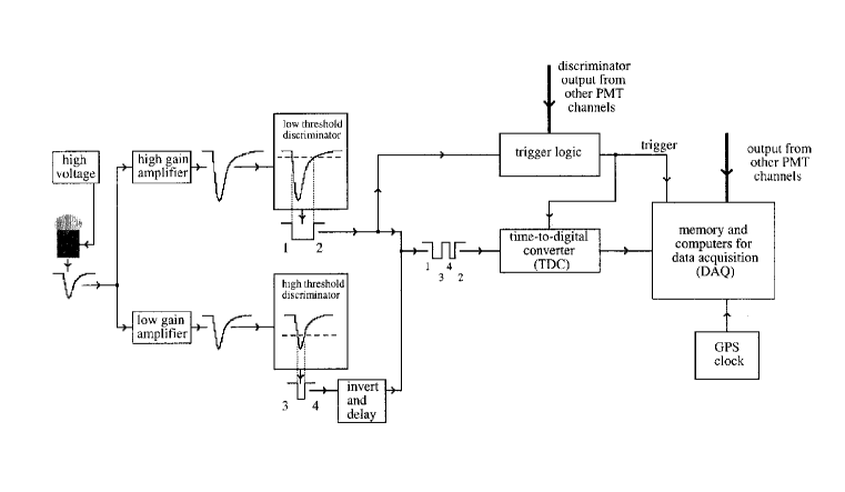
Figure 2: Schematic diagram of a PMT channel.

4 Timing Edges.

Time-over-threshold pulses generated by both discriminators (if crossed) are multiplexed into a series of time edges. (Figure 3) It is the polarity and time of these edges which is being recorded as raw data from a PMT. Strong hits cross both thresholds and result in a 4-edge event, weak ones cross low threshold only and produce 2 timing edges.

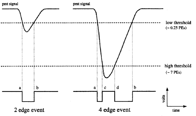
Figure 3: Timing edges.

In practice many edge events can be observed. One edge events can result when the other edge (or edges) is truncated by the trigger time window. Four edge events can be a sequence of two 2-edge events. Multi edge hits are also possible. A filtering algorithm had been designed to clean the hits. It bases its decisions on the polarity of hits and their relative time separation. On average, about 8% of PMT hits are rejected as having invalid edge sequences. The accepted PMT hits are characterized by start time (LoStart) and time over low threshold (LoTOT) and their high threshold counterparts (HiStart, HiTOT) if available.

5 Monte Carlo Simulation of the Detector.

The simulation of the detector response is done in two steps: (1) initial interaction of the primary particle (proton or photon) with the atmosphere and the subsequent generation of secondary particles, and (2) detector response to the secondary particles reaching the detector level. The CORSIKA [23] air-shower simulation code provides a sophisticated simulation of secondary particle development in the Earth’s atmosphere induced by a primary particle with energy up to $10^{20}$ eV. Within CORSIKA, the VENUS code is used to treat hadron-nucleus and nucleus-nucleus collisions at high energies whereas GHEISHA is used at low energies ($<80$ GeV). Electromagnetic interactions are simulated using EGS 4 code. The atmosphere adopted in CORSIKA consists of nitrogen, oxigen and argon in volume proportions of 78.1%, 21.0% and 0.9% respectively. The density variation of the atmosphere with altitude is modeled by 5 layers. In CORSIKA a flat atmosphere is adopted which is a good approximation up to zenith angles of about $70^{\circ}$ where discrepancy with the shperical one reaches one radiation length.

The simulation of the detector itself is based on GEANT [24]. All of the secondary particles in a shower cascade reaching the Milagro are used as input to the GEANT with uniform random placement of the shower core around the detector. GEANT simulates the electromagentic and hadronic interactions of particles in the pond and results in the set of simulated times and pulse heights at each PMT. This information is saved in the same format as the real data and is used to establish properties of the detector. The detailed simulation of the electronics and phototubes continues to be the area of active reseach. Further improvements and understanding are expected.

Chapter 4 Calibration.

1 System Setup and Goals.

The calibration system has been designed to reflect the physics goals of the detector and is used to obtain parameters needed to transform the raw counts to physically meaningful arrival times and light intensities which then can be used for event reconstruction. Despite the considerable effort that has been made to construct all PMT channels of the detector as uniformly as possible, in order to achieve the high precision required for the event reconstruction the remaining variations between channels have to be compensated for. A separate set of calibration parameters is determined for each PMT channel.

The desire to determine the positions of events on the Celestial Sphere with systematic errors much less than the expected angular resolution (which is about $1^{\circ}$) dictates that the locations of the photo-tubes be known to about 10 cm accuracy in horizontal direction and 3 cm in vertical, and PMT timing accuracy to about 1 ns. Photographic and theodolite surveys were used to ensure accurate PMT position determinations.

To achieve the stated time accuracy it is important to calibrate the TDC conversion factors, compensate for pulse amplitude dependence of TDC measurements (known as slewing correction) and synchronize all TDCs (find TDC time off-sets) to the required accuracy. Time over threshold to photo-electron conversion must be determined to convert all PMT amplitude measurements to a common unit for each event. All of the above is achieved with the help of the laser calibration system.

The calibration system is based on the laser—fiber-optic–diffusing ball concept used in other water Cherenkov detectors [25]. A computer operated motion controller drives a neutral density filter wheel to attenuate a 300 picosecond pulsed nitrogen dye laser beam. The selected dye emitted light at 500 nm. The beam is directed to one of the thirty diffusing laser balls through the fiber-optic switch (see figure 1). Part of the laser beam is sent to a photo-diode. When triggered by the photo-diode, the pulse-delay generator sends a trigger pulse to the data acquisition system. A laser fire command is issued by the motion controller, providing full automation of the calibration process. The balls are floating in the pond so that almost every PMT can be illuminated by more than one light source. Complete description, operation, analysis, problems and suggestions are described in [29].

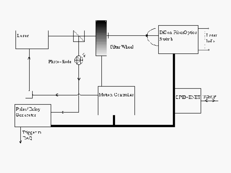
Figure 1: Calibration system setup.

2 Timing Calibration.

1 Slewing Calibration.

Time slewing is the dependence of the reaction time of a PMT together with its electronics on the intensity of the incident light. The amount of light in the calibration system is regulated by the filter wheel whose transmission property ranges from completely opaque to completely transparent thus enabling the study of the effect. The ideal situation of no slewing should reveal itself as independence of PMT registration times with respect to photo-diode when intensity of light in the calibration system is changed.

In practice, it takes longer for weak pulses to cross a discriminator threshold, and thus results in a delay. This is illustrated on the figure 2.

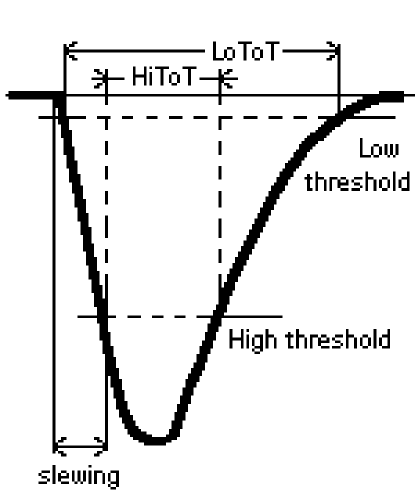
Figure 2: Slewing and Time over Threshold. The weaker the pulse (or, equivalently, the higher the discriminator threshold) the latter the registration time is. Infinitely large pulse will cross the threshold without any delay, or zero slewing.

Because the light intensity is characterized by time over threshold, the amount of slewing is studied with respect to this variable. The method of generation of such a slewing curve is explained with the help of the figure 3.

Figure 3: Conceptual drawing of a measurement performed for timing calibration.

This diagram is high/low threshold independent, the scheme is applied independently for both threshold levels. The slewing curve is a plot of $T_{start}$ vs $ToT$. Note, that $T_{start}$ includes the propagation time of pulses in the water and in the optical fiber, delays associated with the details of the particular PMT channel and common detector trigger delays. Because common offsets are irrelevant, after correcting for relative fiber delays and water propagation times which effectively shifts the curve up or down, this will become a complete timing calibration. The slewing correcting curve is found by fitting a polynomial to $T_{start}$ vs $ToT$. If a PMT gets a slewing curve from more than one laser ball, the curve resulting from the maximal light illumination is chosen. An example of a slewing curve is presented in figure 4. The TDC’s used in Milagro employ a common stop, thus larger values of $T_{start}$ correspond to earlier times.

(a) Example of the $T_{start}$ vs $ToT$ data points.

(b) Example of the polynomial fit. The values in each bin are the means of the $T_{start}$ obtained by a fit of a Gaussian distribution in the corresponding $ToT$ bin.

Figure 4: Plots showing a typical data obtained from the calibration system for the purpose of timing calibration. Units of both axis are TDC counts.

2 TDC Conversion Verification.

The time to digital converters measure time in the units of “counts”. According to LeCroy 1887 FASTBUS TDC specifications one count corresponds to 0.5 nanoseconds. This was verified by insertion of known variable delay in the photo-diode trigger chain with the help of DG535 digital delay/pulse generator by Stanford Research Systems. The shift in the start times ($T_{start}$) of all PMTs was found to be very consistent with the 2 count per 1 ns conversion. This assured that all TDC clock speeds are the same and meaningful interpretation of time across all PMT channels is available.

3 Fiber-Optic Delays. Speed of Light in Water.

The last step of timing calibration is correcting the slewing curve for both the light propagation time in water between the PMT and the laser ball used to generate the curve and the relative delay in the fiber attached to that ball. In order to correct for the propagation time, coordinates of PMTs and balls and the speed of light in water have to be given. PMT and laser ball coordinates are known from the survey. (If laser ball coordinates are deemed to be inaccurate, they can be found from the calibration data: see [26, 27].) Because only a typical index of refraction of water is found in reference tables and because fiber-optic delays vary from ball to ball, these parameters have to be evaluated on the basis of the calibration data itself.

The method to solve the problems uses the ability to cross calibrate a PMT using several laser balls. If $T_{1}$ and $T_{2}$ are slewing corrected times registered by a PMT from two laser balls (1 and 2), then the difference $(T_{1}-T_{2})$ does not depend on delays in the PMT electronics (common to both measurements), but instead reflects the difference in propagation times from the corresponding balls and the relative fiber delays. Consider the following quantity:

$$\tau=T_{1}-T_{2}+\Delta_{fiber}+\Delta_{propagation}$$

If speed of light and fiber delays are correct, then $\tau$ is zero within errors of measurement. When for given laser ball pair many PMTs with their $\tau$’s are considered, one sees that for PMTs located approximately half way between the balls $\Delta_{propagation}\approx 0$ and deviation of average $\tau$ from zero is due to fiber delay difference. On contrary, PMTs located in the close proximity of either ball provide information about the speed of light: the usage of incorrect speed of light will widen the distribution of $\tau$’s. Thus the analysis of all $\tau$’s for all PMTs and laser ball pairs enables the determination of speed of light in water and relative fiber delays.

Slewing curves are shifted by the appropriate propagation time and fiber delay to yield the final timing calibration for each PMT.

3 Photo-Electron Calibration.

1 Occupancy Method.

Time over threshold to photo-electron calibration is based on the well-known occupancy method, which was one of the methods of PE calibration of Milagrito [28] and other water Cherenkov detectors [25]. The data used for PE calibration is the same as for the timing calibration which is obtained with the laser light passing through the filter wheel with different transparency settings (which are changed by rotating the wheel). The main task of the PE calibration is determination of the number of photo-electrons for a given incident light intensity (ToT). The basic method consists of two steps: 1. at low light levels calibrate using the occupancy method, and 2. extend to higher light levels using given attenuation properties of the filter wheel.

1. Calibration at low light levels.

   At low light levels it is possible to measure the number of photo-electrons as function of ToT directly. The method is founded on the following assumptions:

   • The number of photo-electrons produced at PMT’s photocathode obeys a Poisson distribution:

     $$P_{\lambda}(n)=\frac{\lambda^{n}}{n!}e^{-\lambda}$$

     where $\lambda$ is the mean number of the photo-electrons produced. (This is justified because the probability of emitting a single photo-electron does not depend on the fact of possible emission of other photo-electrons.)

   • A constant light intensity source is used in calibration.

   Then, the probability $\eta$ that at least one photo-electron was produced while the photocathode was illuminated (the probability that the PMT “saw” the illumination) is called occupancy and is given by:

   $$\eta=P(n>0)=1-P_{\lambda}(n=0)=1-e^{-\lambda}$$

   Occupancy can be easily measured if the PMT is illuminated several times with the same pulse intensity:

   $$\eta=\frac{number\;of\;observed\;pulses}{total\;number\;of\;pulses}$$

   Therefore, if $\eta$ is known, then $\lambda=-\ln(1-\eta)$. This method is applicable at relatively low light levels (when $\lambda<2$) because at high levels the occupancy saturates to 1 and a small measurement error in $\eta$ will lead to a big error in $\lambda$:

   $$\Delta\lambda=\frac{1}{1-\eta}\Delta\eta=e^{\lambda}\Delta\eta$$

2. Calibration at high light levels.

   Calibration at high light levels is achieved by noting that in the absence of PMT/electronics saturation the number of photo-electrons is proportional to the light intensity at the photocathode. If the transmittance of the filter wheel $T$ is known, then:

   $$\lambda=aT$$

   where $a$ is some coefficient which is different for each laser ball PMT pair. This coefficient can be found at low light levels where $\lambda$ is also known. Error of this method will grow linearly with light intensity, not exponentially as in low light level case. Thus, given transmittance $T$ of the filter wheel, ToT-to-PE conversion can be achieved at any light level. When, in reality, saturation is present prescribing the number of photo-electrons using this as a requirement allows protection against the effect. Traditional amplitude-to-digital conversion methods which make use of the air shower data are susceptible to such non-linearity.

2 In Situ Filter Wheel Calibration.

Traditionally, filter wheel calibration is obtained either from the manufacturer or by a separate measurement. In Milagro, in situ filter calibration method was developed which uses the same calibration data. The idea is grounded on the supposition that for any two sufficiently close levels of transmittance of the filter wheel ($T_{1}$ and $T_{2}$) there exists a PMT in the pond for which the occupancy method is valid on both light intensities. If $\lambda_{1}$ and $\lambda_{2}$ are corresponding photo-electron measurements, then:

$$\frac{T_{2}}{T_{1}}=\frac{\lambda_{2}}{\lambda_{1}}$$

This line of arguments is used to relate $T_{3}$ to $T_{2}$, $T_{4}$ to $T_{3}$ and so on, leading to restoration of the transmittance levels for the entire wheel. Because absolute transmittance of the wheel is irrelevant one can always set $T_{0}=1$.

3 Dynamic Noise Suppression.

Small amounts of radioactive elements present in the water, ambient light, Cherenkov light produced by the shower particles or thermo-electron emission cause signals on the output of PMT channels which constitute noise hits. The presence of these hits will lead to overestimation of occupancy implied by the laser light level and thus will damage the accuracy of the calibration. Dynamic noise suppression is a technique allowing the solution of this problem on the tube by tube basis.

An event, registered by a PMT could have come from a laser pulse or from a noise hit which are independent, therefore the probability of observing a hit $P(any)$ is given by:

$$P(any)=P(laser+noise)=P(laser)+P(noise)-P(laser)\cdot P(noise)$$

where $P(laser)$ is probability of observing a pulse due to laser (true occupancy), $P(noise)$ is probability of observing a pulse due to noise. $P(any)$ is measured by sending laser pulses into the pond, $P(noise)$ is obtained by sending “random” (no laser light) triggers to the data acquisition system, then the occupancy is given by:

$$\eta=P(laser)=\frac{P(any)-P(noise)}{1-P(noise)}$$

This is indeed how occupancy was determined for the filter wheel calibration and for the ToT-to-PE conversion. To demonstrate the importance of the suppression refer to figure 5 which shows filter wheel calibration curves obtained with and without noise suppression.

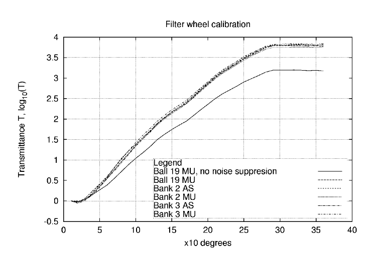
Figure 5: Filter wheel calibration curves obtained with different laser ball — PMT combinations are presented. Bank 2,3 represent laser balls 11-20 and 21-30 respectively. AS, MU — PMT’s of air shower and muon layers respectively. Calibrations with ball 19 and muon layer PMT’s are also shown with and without the noise suppression to illustrate its importance.

4 Slewing Extrapolation.

The maximum light level at which a PMT was calibrated depends on the distances to the laser balls, laser light output and the calibration system optics alignment. The range of $ToT$ within which a tube is calibrated may be too narrow to allow interpretation of the strongest hits generated by the shower particles. The desire to make use of these hits requires extrapolation of the calibration curves beyond the measured points by some plausible functional form. The functional shape depends on the PMT discriminator threshold level, amplification coefficients and so on. Instead of trying to make physical model of the channel a statistical approach is followed.

It is believed that all PMT channels were manufactured to meet common characteristics. Therefore, the study of the channels’ responses (calibration) can be viewed as a multiple (about 700 times, broken PMTs do not count) measurement of a single function of $ToT$. The fact that the calibration curves obtained for different channels are slightly different can be attributed to the “manufacturing imperfections” (such as unavoidable uncontrollable spread of characteristics of electronic components) and can be treated as such.Thus, the curves for all PMTs can be viewed as particular realizations of the same random function [30].

Inasmuch as a random function is a mathematical concept of great complexity and in most general case it can be regarded as a non-denumerable set of scalar random variables, it is natural to seek the expression of the random function in terms of simpler random concepts: ordinary scalar random variables. Therefore, the following representation of the calibration curve $X(t)$ is tried (here $t$ or $t^{\prime}$ denote $ToT$):

$$X(t)=m(t)+\sum_{\nu=1}^{n}V_{\nu}\phi_{\nu}$$

Here, $\{\phi_{\nu},\nu=1,..,n\}$ are some non-random functions, $\{V_{\nu}\}$ are random variables. This representation is said to be canonical if $m(t)$ is the mean function ($m(t)=M[X(t)]$) and $V_{\nu}$’s are uncorrelated with zero mean [31]:

$$M[V_{\nu}]=0,\;\;\;D[V_{\nu}]=M[(V_{\nu})^{2}]=D_{\nu}$$

$$M[V_{\nu}\cdot V_{\mu}]=0\;\;\;\mu\neq\nu$$

When such a representation is found, each particular calibration curve $x(t)$ can be extrapolated using the expansion and the set of coefficients $v_{\nu}$ can be calculated in the range where calibration data is available. The construction of the canonical representation makes use of the average function $m(t)$ and the correlation function $K(t,t^{\prime})=M[X^{\circ}(t)\cdot X^{\circ}(t^{\prime})]$, where $X^{\circ}(t)=X(t)-m(t)$. It can be shown that

$$\phi_{\mu}(t)=\frac{1}{D_{\mu}}\sum_{k=1}^{m}a_{\mu k}K(t,t_{k})$$

$$V_{\mu}=\sum_{k=1}^{m}a_{\mu k}X^{\circ}(t_{k})$$

satisfy the conditions of the canonical representation if coefficients $a_{\mu k}$ are chosen such that

$$\sum_{k,l=1}^{m}a_{\mu k}a_{\nu l}K(t_{k},t_{l})=0\;\;\mu\neq\nu$$

which is always possible if the number $m$ of sample points $\{t_{k}\}$ is large enough ($m>(n-1)/2$) [32]. The root mean square deviation of the representation from the realization is given by:

$$rms(t)=\sqrt{K(t,t)-\sum_{\mu=1}^{n}D_{\mu}(\phi_{\mu}(t))^{2}}$$

This scheme is used for extrapolation of slewing curves of timing calibration. It is implemented to the first order of the canonical expansion [32]. The only sample point $t_{1}$ is the highest value of $ToT$ available from the calibration data. Therefore, the extrapolation is obtained by:

$$x(t)=m(t)+\frac{x(t_{1})-m(t_{1})}{K(t_{1},t_{1})}K(t,t_{1})$$

The typical extrapolation range needed to interpret shower data is less than 100 ns in $ToT$ leading to the error of the extrapolation being less than 0.7 ns [32]. Comparison of the extrapolated curves and measured ones obtained in different calibration runs yielded the measured extrapolation error of 0.55 ns [33] in good agreement with the expectations.

Chapter 5 Event Reconstruction.

1 Primary Particle Direction Reconstruction.

The data registered in each event is used to infer the characteristics of the primary particle that created the shower: its direction of incidence, energy and type. In order to be able to make the inference about the properties of the primary particle based on the observed quantities one has to assume the relation between the two. One of these relations is expressed by equation 2, the lateral distribution of the shower. If the arrival direction is known, then the depth $t$ of the atmosphere traversed by the shower can be determined from geometrical consideration and then, equation 1 together with equation 2 relate the measured lateral distribution $\rho(r)$ with energy of the primary particle and shower core position. From the practical point of view, the fluctuations in the shower development, small size of the detector and fluctuations in its response make this program infeasible [34]. The detector is currently being upgraded with the array of water tanks which will aid in core location, allowing achievement of 30% energy resolution [34].

The task of determination of the primary particle direction is much simpler and is of highest importance (from the gamma ray astronomy point of view). The basic idea is as follows. Let us assume that the shower front is a plane, perpendicular to the direction of motion of the primary particle. Then, as in any air shower array, each detector $i$ in the set records the local arrival time $T_{i}$ of the shower front (see figure 1) which has to be contrasted with the model: a plane defined by a normal vector $\vec{n}=(a,b,c)$, the direction of the primary particle:

Figure 1: Schematic diagram of a shower array detectors and how timing information can be used to determine the direction of the primary particle $\vec{n}$. Lines represent measured arrival times, filled circles — the locations of detectors.

$$T_{i}=\frac{ax_{i}+by_{i}+cz_{i}}{v_{0}\sqrt{a^{2}+b^{2}+c^{2}}}+T_{0}$$

where, $(x_{i},y_{i},z_{i})$ are coordinates of PMT $i$, $v_{0}$ — is the speed of the shower front in air, $T_{0}$ — is a common time offset for the whole event. Noting that Milagro is a flat array, thus $z_{i}\equiv 0,\forall i$, and introducing notations:

$$A=\frac{a}{v_{0}\sqrt{a^{2}+b^{2}+c^{2}}},\;\;\;B=\frac{b}{v_{0}\sqrt{a^{2}+b^{2}+c^{2}}}$$

we obtain the final model

$$T_{i}=Ax_{i}+By_{i}+T_{0}$$

When coefficients $A$ and $B$ are found, the direction of the incoming shower is reconstructed as

$$\left\{\begin{array}[]{rcl}\cos(\phi)&=&\frac{A}{\sqrt{A^{2}+B^{2}}}\\ \sin(\phi)&=&\frac{B}{\sqrt{A^{2}+B^{2}}}\\ \theta&=&\arcsin(v_{0}\sqrt{A^{2}+B^{2}})\end{array}\right.$$

where $(\theta,\phi)$ are zenith and azimuth angles, and $v_{0}$, the speed of the shower front in air, is approximately equal to the speed of light.

The method of determination of coefficients $A$ and $B$ from the measured times $T_{i}$ is a $\chi^{2}$ fit where weights are chosen based on the recorded light intensity of the PMTs. This is because more energetic particles appear to suffer less fluctuations due to the combined effect of the shower development and PMT time resolution and thus are given higher weight. The weights were derived by studying the distributions of $T_{i}$’s [35]. These distributions are not Gaussian, as assumed by the $\chi^{2}$ fit, therefore, several iterations are made. The experimental points are also occasionally just way off (such as times of incidental hits). Points like this are called outliers. They can easily turn a $\chi^{2}$ fit on otherwise adequate data into nonsense. Their probability of occurrence in the assumed Gaussian model is so small that the estimator is willing to distort the whole curve to try to bring them, mistakenly, into line. Therefore, on the first iteration only PMTs with hits of greater than 2 PE are used. On the next iterations the PE restriction is gradually relaxed so that PMTs with weaker signals are allowed to participate. At the same time, the definition of outliers becomes more stringent. After the first iteration points with distance of more than two standard deviations away from the plane are removed from the fit on the second pass. Before the last, fifth, pass outliers are defined as all hits with distance of more than 0.5 standard deviations away from the plane. The results of the last iteration are recorded as the reconstructed direction of the primary particle. The number of PMTs that participated in the last pass are also noted as $N_{fit}$.

More sophisticated algorithms were also attempted, they, however, required a significantly higher computer power without improving angular resolution by a noticeable amount [36]

2 Core Location.

The inability to make precise determination of the shower core impacts not only energy estimation but also the direction reconstruction. Indeed, as was mentioned in section 3, the shower front is not flat, but rather presents a paraboloid surface. Therefore, in order to be able to use the described plane fit algorithm, the shower front has to be “unfolded” into the plane. The amount of this curvature correction is certainly core distance dependent. Failure to apply curvature correction will result in a systematic error in the direction reconstruction which increases with core displacement from the pond. Because there are many showers with different core positions, this will lead to degradation of average angular resolution.

Thus, for the purposes of angle determination, the following core locating algorithm was adopted [37]. First the direction to the core from the center of the pond is determined by calculating the location of the provisional core. The provisional core position is found in two iterations. Iteration one: the average PMT coordinate is calculated where the weight is taken to be $\sqrt{PE}$ of the corresponding PMT. The second iteration is the same as the first, but where only PMTs within $\pm 45^{\circ}$ sector of the direction found on the iteration one are used. After the provisional core is found, the decision is made whether the shower core is on the pond or it is outside of it. The decision is made on the basis of profile of the average PE versus distance from the center of the pond for PMTs within $\pm 60^{\circ}$ sector of the provisional core direction. If it is declining sufficiently fast towards the edge of the pond, the core is adopted to be on the pond. Otherwise, it is off. On-pond cores are found as $PE$ weighted average of PMT coordinates in the circle of 8 meters around provisional core. Off-pond cores are placed at a distance of 50 meters from the center of the pond in the direction defined by the provisional core. Only PMTs of the shower layer are used in this algorithm. The value of 50 meters is chosen because simulations indicate that this is the most probable core displacement for showers triggering the detector.

In the early part of the detector running, a more primitive version of the algorithm was used.

3 Curvature Correction.

The origin of the curvature correction is traced back to the desire of using the plane model of the shower front in the direction reconstruction and to the details of the shower development underlined in section 3: the shower front is parabolic. It was shown that electron and photon components of the shower have different shapes of the corresponding fronts (figure 3). This means that the shape of the front, as sampled by the array, depends on energy threshold of the detectors and on the relative efficiency for photon conversion. For this reasons, methods of determination of the curvature correction from the real data were developed [35]. A particular representation of the correction was chosen and then parameters were optimized in a multistage iteration process. The correction was shown to improve angular resolution compared to a plane fit.

4 Sampling Correction.

The curvature correction and core finding algorithms provide for primary particle direction reconstruction given that the times of the arrival of the shower front are measured by the detectors. However, as was mentioned in section 2, each PMT has quantum efficiency of about $0.2-0.25$. This means that the first particle, carrying information about the shower front, is detected with some probability $p$. If this particle is missed, the tube is presented a chance of detecting the second particle in the shower and so on up to the total number of particles $\rho(r)dxdy$ which make up the thickness of the front at the specific core distance $r$. Thus, if $f_{n}(T,r)$ is the time distribution of the $n$-th particle, $f_{1}(T,r)$ being the shower front, then the distribution $g(T,r)$ of the detected arrival times is given by:

$$g(T,r)=pf_{1}(T,r)+(1-p)pf_{2}(T,r)+\dots+(1-p)^{n-1}pf_{n}(T,r)+\dots$$

If nothing else is known, the $g(T,r)$ has to be interpreted as the shower front instead of $f_{1}(T,r)$. This would certainly lead to poorer angular resolution. The Milagro analysis tries to exploit the correlation that particles trailing the front are of monotonously decreasing energy, making it possible, effectively, to estimate the order number $n$ of the detected particle. With regard to the core distance dependence, each of the $f_{n}(T,r)$ is narrower where density of particles $\rho(r)$ is higher, that is towards the core. Thus, the sampling correction is aimed at inferring the arrival time of the front needed for direction reconstruction, it is due to finite detection efficiency of the PMTs and it is a function of core distance and light intensity registered by the PMT. Such estimated front arrival times are subject to higher fluctuations compared to direct measurements and therefore are given less weight in the direction reconstruction algorithm [35].

5 Cosmic Ray Rejection.

The identification of the type of the primary particle (photon or cosmic ray) in Milagro makes use of the presence of muons and hadrons in cosmic-ray initiated cascades. In the top layer of the detector their presence is obscured by the general illumination by the shower particles, in the bottom layer, however, they may be noticed. Penetration of one of these particles to the muon layer should lead to clusters of high light intensities. In the case of a primary photon, the illumination of the bottom layer should be uniform. It was found with the help of Monte Carlo simulations that the parameter $X_{2}$ defined as

$$X_{2}=\frac{N_{2}}{PEmax}$$

is sensitive to the type of the primary particle. Here $N_{2}$ is the number of PMTs in the muon layer with registered light intensities greater or equal to 2 PE, PEmax — is the maximum intensity detected in the event by the muon layer ([38] and [39]). The simulated distributions of parameter $X_{2}$ for gamma- and proton- induced showers are presented on figure 2. The $X_{2}$ distribution for the proton dominated data (also shown on figure 2) agrees with the simulated proton distribution well. This match is a check of the Milagro Monte Carlo simulations.

Figure 2: Distributions of parameter $X_{2}$. Dashed line is Monte Carlo simulations for photon induced showers, dotted line is simulation for proton induced showers, solid line is the data. Each distribution is normalized to 1.

It is clear that events with large values of the parameter are more likely to be gamma ray induced. It was determined that the optimal cut for gamma rays is accepting events with $X_{2}>2.5$. At this cut, about 90% of protons are rejected while about 50% of gamma rays are accepted.

Attempts to develop a more complicated criterion have not yet yielded a significant improvement over the present scheme.

Chapter 6 Performance of the Milagro Detector.

1 Operation of the Milagro.

The Milagro detector operates largely unattended in a reliable and stable manner. Automatic alerts are generated under serious error conditions such as loss of electrical power, an abnormal event rate, or overheating of the electronics. The nature of the error, time of the day and weather conditions determine the response time and restart of the data taking. Less serious problems can be corrected remotely. There are also scheduled down times to accommodate repair activities and calibrations. Other than that, data are acquired continuously. During operation of the detector some PMT-electronics channels cease to work and have to be turned off. This problem has typically been traced to water leakage of the under-water connectors linking coaxial electric cable with the PMT. Repairs of these connectors performed once a year are a major part of the scheduled maintenance down time. The repair time is chosen to be September when the pond water is the warmest to facilitate the scuba diving to retrieve PMTs.

2 Angular Resolution.

The cosmic ray shadow of the Moon has been used to measure the angular resolution of an EAS array above 50 TeV [40]. At TeV energies, the geomagnetic field will displace the Moon cosmic ray shadow. Another estimate of the angular resolution is obtained by studying $\Delta_{eo}$ — the difference between directions reconstructed by the same “color” PMTs if the detector is imagined to be painted in the white and black squares of a checkerboard. (The PMT numbering scheme was designed in such a way that the color of the PMT is defined by the parity (even/odd) of its number.) The quantity $\Delta_{eo}$ is not sensitive to certain systematic effects, common to the both parts of the detector, however, in the absence of these effects the dispersion of $\Delta_{eo}$ is twice the overall angular resolution [41]. From the studies of the Moon shadow, the $\Delta_{eo}$ and the Monte Carlo simulations, the estimated angular resolution of the instrument including pointing effects is $0.75^{\circ}$ for all events with $N_{fit}>20$.

3 Absolute Energy Scale.

The absolute energy scale can be determined by examining the magnetic displacement of the shadow of the Moon. A preliminary estimate of the median energy of the detected events is $640\pm 70$ GeV which is in excellent agreement with simulations which predict median energy of 690 GeV.

4 Cosmic Ray Rejection at Work.

All observations to date indicate that the flux of gamma rays from the Crab nebula is constant which makes it a very useful source for testing the sensitivity of different instruments. The cosmic ray rejection method was tested on the Crab. If the data is analyzed without application of the $X_{2}$ cut, the Crab is observed with significance of 1.4. Analysis of the data passing the rejection criterion yields significance of 5.4. (The notion of significance is discussed in section 2.) The data set used in this study covers the period between June 8, 1999 and April 1, 2002 [42].

Chapter 7 Data Analysis Technique.

1 Coordinate Systems on the Celestial Sphere.

1 Equatorial Coordinate System.

Inasmuch as distances to the majority of astronomical objects are much bigger than the size of the Earth and its orbit, it is sufficient to specify directions to the objects regarding distances as equal and infinitely large. Within this framework, the stars appear to be located on the surface of an imaginary sphere with the observer at its center. This sphere is called the Celestial sphere. Various coordinate systems on the sphere are used, all defined by the corresponding choices of reference circles. Horizon and equatorial coordinate systems are important examples employed in this work [43]. Figure 1 illustrates the following definitions.

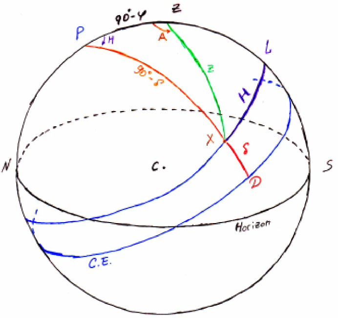
Figure 1: Definitions of horizon and equatorial coordinate systems.

$C$

- the observer.

$CP$

- line parallel to the axis of rotation of the Earth.

$P$

- North celestial pole.

Celestial Equator

- is defined as intersection of a plane perpendicular to $CP$ at point $C$ and the celestial sphere. (This is the projection of Earth’s equator.)

$Z$

- the zenith, intersection of the celestial sphere with the outward continuation of the plumb line at the observer’s location.

$\angle PCZ=90^{\circ}-\phi$

- definition of $\phi$. Angle $\phi$ is astronomical latitude of the observer on the Earth.

Horizon

- is defined as intersection of a plane perpendicular to $CZ$ at point $C$ and the celestial sphere.

$N,S$

- are North and South of the Horizon. $N$ and $S$ are defined as the intersection of a great circle $PZ$ centered at observer $C$ with the Horizon. Arc $PZLS$ is called local reference celestial meridian.

$X$

- is a star.

$\angle ZCX=\stackrel{{\scriptstyle\smile}}{{ZX}}=z$

- zenith distance of star $X$.

$A$

- azimuth, is a dihedral angle between reference meridian and $ZXC$ plane.

$\angle LCX=\stackrel{{\scriptstyle\smile}}{{LX}}=H$

- hour angle, is a dihedral angle between reference celestial meridian and that of the star $PXD$.

$\angle XCD=\stackrel{{\scriptstyle\smile}}{{XD}}=\delta$

- is Declination of a star (Dec.).

The equatorial coordinate system of hour angle and declination $(H,\delta)$ is built around the axis of rotation of the Earth whereas the horizon one of zenith and azimuth $(A,z)$ uses a plumb line as the reference. The law of cosines for trihedral angles applied to the spherical triangle $XPZ$ (figure 1) two times yields the relation between the systems:

$$\cos(90^{\circ}-\delta)=\cos z\cos(90^{\circ}-\phi)+\sin z\sin(90^{\circ}-\phi)\cos A$$

$$\cos z=\cos(90^{\circ}-\delta)\cos(90^{\circ}-\phi)+\sin(90^{\circ}-\delta)\sin(90^{\circ}-\phi)\cos H$$

or,

$$\sin\delta=\sin\phi\cos z+\cos\phi\sin z\cos A$$

$$\tan H=\frac{\sin z\sin A}{\cos\phi\cos z-\sin z\sin\phi\cos A}$$

The value of observer’s latitude $\phi$ defined as the complement of the angle $\angle PCZ$ is assumed to be known. Both of these coordinate systems are local coordinate systems in the sense that both of them revolve with the Earth. If the object $X$ is stationary in space, due to the Earth’s rotation it will appear to be moving and its local coordinates will be changing. With this motion, the declination $\delta$ of the stationary object in the equatorial system will remain constant, while its hour angle $H$ will change incrementing by $360^{\circ}$ when the Earth makes one full revolution around its axis $CP$. The time required to complete such a revolution is called sidereal day. In contrast, the solar day or universal day is defined as the time between two appearances of the Sun on the local reference celestial meridian. The universal time is different from the sidereal time due to Earth’s orbital motion around the Sun.

Equatorial celestial coordinate system is defined as declination $\delta$ and right ascension $\alpha$ of the object, where $\alpha=H_{\Upsilon}-H$, $H_{\Upsilon}$ is the hour angle of the vernal equinox. This coordinate system is independent of the Earth’s rotation and observer’s longitude. Local sidereal time is defined as $H_{\Upsilon}$ expressed in the units of time.

Local sidereal time as well as the geodesic latitude of Milagro are provided by the GPS system clock. In general, there is no exact relation between astronomical latitude defined above and the geodesic one, but according to indications in literature [44] the difference is of the order of $15^{\prime\prime}$ in magnitude, much smaller than the angular resolution of the detector and thus can be neglected.

2 Galactic Coordinate system.

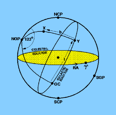
Figure 2: Definition of Galactic coordinate system in its relation to the equatorial coordinate system.

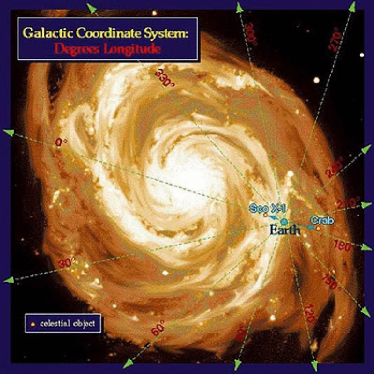
(a) View of the Galaxy from the North Galactic pole. Galactic longitude grid is shown. The Galaxy, at the Earth’s position, is rotating toward the direction of $l=90^{\circ}$.

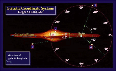
(b) Side view of the Galaxy. Galactic latitude grid is shown. The arrow indicates the direction of increment of Galactic longitude which is opposite to the Galactic rotation.

Figure 3: Artist view of the Milky Way Galaxy from aside.

The reference plane of the galactic coordinate system is the disc of our Galaxy (i.e. the Milky Way) and the intersection of this plane with the celestial sphere is known as the galactic equator, which is inclined by about $63^{\circ}$ to the celestial equator. Galactic latitude, $b$, is analogous to declination, but measures distance north or south of the galactic equator, attaining $+90^{\circ}$ at the north galactic pole (NGP) and $-90^{\circ}$ at the south galactic pole (SGP). The galactic latitude of the star X on the figure is arc YX and is north (figure 2).

Galactic longitude, $l$, is analogous to right ascension and is measured along the galactic equator in the same direction as right ascension. The zero-point of galactic longitude is in the direction of the Galactic Center (GC), in the constellation of Sagittarius; it is defined precisely by taking the galactic longitude of the north celestial pole to be exactly $123^{\circ}$. The galactic longitude of the star X on the figure is given by the angle between GC and Y.

The galactic north pole is at RA = 12:51.4, Dec = +27:07 (2000.0), the galactic center at RA = 17:45.6, Dec = -28:56 (2000.0). The inclination of the galactic equator to Earth’s equator is thus $62.9^{\circ}$. The intersection, or node line of the two equators is at RA = 18:51.4, Dec = 0:00 (2000.0), and at $l=33^{\circ}$, $b=0^{\circ}$ [45]. Transformation between celestial coordinate system and galactic one are given, therefore, by [46]:

$\cos b\cos(l-33^{\circ})$	=	$\cos\delta\cos(\alpha-282.85^{\circ})$
$\cos b\sin(l-33^{\circ})$	=	$\cos\delta\sin(\alpha-282.85^{\circ})\cos 62.9^{\circ}+\sin\delta\sin 62.9^{\circ}$
$\sin b$	=	$\sin\delta\cos 62.9^{\circ}-\cos\delta\sin(\alpha-282.85^{\circ})\sin 62.9^{\circ}$

2 Significance of a Measurement.

According to its definition [47], a statistical hypothesis is a theoretical prediction or assertion about the distribution of one or several measurable quantities. It is therefore desired to devise a rule of checking whether the data are consistent with the hypothesis, called null hypothesis $H_{0}$. Such a rule, however, can not be hoped to tell whether the hypothesis is true or false, it can only insure that in the long run of experience wrong propositions will not be accepted too often. A naive method of testing is to calculate the probability that a certain character $x$ of the observed data would arise if $H_{0}$ were true. If the probability is small, this is considered as an indication that the hypothesis is false and it is rejected. However, if $x$ is a continuous variable, then probability of any value of $x$ is zero. Therefore, tests are based on the notion of critical region. The critical region $w$ is the subset of space $W$ of all possible values of $x$ such that $x$ falling into $w$ leads to the rejection of the hypothesis. The hypothesis is accepted or remains in doubt in all other cases. It follows then, that if there are two alternative tests for the same hypothesis, the difference between them consists in the difference in critical regions. It also follows that $H_{0}$ can be rejected when, in fact, it is true (error of the first kind); or it can be accepted when some other alternative hypothesis $H_{1}$ is true (error of the second kind). (Admittance of the existence of an alternative hypothesis is clear, otherwise the null hypothesis would not be questioned.) The probabilities of errors of these two kinds depend on the choice of the critical region. The critical region is said to be the best for testing hypothesis $H_{0}$ with regard to $H_{1}$ if it is the one which minimizes the probability of the error of the second kind among all regions which give the same fixed value of the probability of the error of the first kind. The construction of the best critical region, resulting in the most efficient test of $H_{0}$ with regard to $H_{1}$ was considered by Neyman and Pearson in [47]. The problem is solved for the general case of simple hypotheses. A hypothesis is said to be simple if it completely specifies the probability of the event; it is composite if the probability is given only up to some unspecified parameters.

Critical regions $w(\epsilon)$ corresponding to different probabilities $\epsilon$ of errors of the first kind are engineered before the test is performed. When experimental data $x$ is obtained, the smallest $\epsilon$ is found such that $x\in w(\epsilon)$. It is then said, that based on the experimental data, the null hypothesis can be rejected with significance $\epsilon$.

A typical astronomical experiment consists of two independent observations of some regions of the sky yielding two measured counts $N_{1}$ and $N_{2}$ made during time periods $t_{1}$ and $t_{2}$ respectively with all other conditions being equal. The null hypothesis being tested is that $N_{1}$ and $N_{2}$ constitute a sample of size 2 from a single Poisson distribution (adjusted for the duration of observations) which is due to common illumination. The alternative is that the two measurements are due to Poisson distributions with unrelated parameters. In other words, the alternative hypothesis $H_{1}$ is of the form:

$$H_{1}:\;\;p_{1}(N_{1},N_{2})=\frac{(\lambda_{1}t_{1})^{N_{1}}}{N_{1}!}e^{-\lambda_{1}t_{1}}\frac{(\lambda_{2}t_{2})^{N_{2}}}{N_{2}!}e^{-\lambda_{2}t_{2}}$$

while the null hypothesis is also of the composite type, obtained from the $H_{1}$ by setting $\lambda_{1}=\lambda_{2}$:

$$H_{0}:\;\;p_{0}(N_{1},N_{2})=\frac{(\lambda t_{1})^{N_{1}}}{N_{1}!}\frac{(\lambda t_{2})^{N_{2}}}{N_{2}!}e^{-\lambda(t_{1}+t_{2})}$$

that both measurements are due to the same unknown count rate $\lambda=\lambda_{1}=\lambda_{2}$.

Despite the fact that $p_{0}(N_{1},N_{2})$ admits the existence of regions similar to the sample space $W$ with regard to the parameter $\lambda$, no common best critical region with the respect to every alternative admissible $(\lambda_{1}\neq\lambda_{2})$ hypothesis $p_{1}(N_{1},N_{2})$ can be found.

Therefore, the following practical method is adopted which is to consider

$$S=\frac{N_{1}-\alpha N_{2}}{\sqrt{N_{1}+\alpha^{2}N_{2}}},\;\;\;\;\;\alpha=t_{1}/t_{2}$$ (1)

Arguments can be made (appendix 12) that for large $N_{1}$ and $N_{2}$, under the null hypothesis, $S$ obeys the standard normal distribution in the vicinity of zero. The bounds of this approximation $-S_{0}<S<S_{0}$ enlarge when smallest of the $N$’s increases (equation 1). The critical regions $w(\epsilon)$ with respect to the alternative hypothesis $\lambda_{1}>\lambda_{2}$ are, therefore, defined as $S>S(\epsilon)$, where:

$$\epsilon=\frac{1}{\sqrt{2\pi}}\int_{S(\epsilon)}^{\infty}e^{-\frac{x^{2}}{2}}dx$$

and provide the way to calculate the significance of the measurement $\epsilon$. (The critical regions $w(\epsilon)$ with respect to the alternative hypothesis $\lambda_{1}<\lambda_{2}$ are defined as $S<S(\epsilon)$, $\epsilon=\frac{1}{\sqrt{2\pi}}\int_{-\infty}^{S(\epsilon)}e^{-\frac{x^{2}}{2}}dx$.) Because of the one-to-one correspondence between $\epsilon$ and $S(\epsilon)$, the significance of a measurement can be quoted in the units of $S$ (see table 1). The error on the value of $\epsilon$ due to this approximation is less than $\frac{1}{\sqrt{2\pi}}\int_{S_{0}}^{\infty}e^{-\frac{x^{2}}{2}}dx$.

$|S(\epsilon)|$	$\epsilon$
1.0	0.15866
2.0	0.02275
2.5	$6.21\cdot 10^{-3}$
3.0	$1.35\cdot 10^{-3}$
3.5	$2.326\cdot 10^{-4}$
4.0	$3.17\cdot 10^{-5}$

Table 1: The correspondence between $|S|$ and $\epsilon$ for the alternative hypothesis $\lambda_{1}>\lambda_{2}$ or $\lambda_{1}<\lambda_{2}$ [48].

3 Effective Area.

Considering the detector and the atmosphere together as parts of a giant apparatus, it is obvious that not all particles entering the atmosphere will trigger the detector. (Particles on the other side of the Earth will not be registered by the detector.) Thus, it is meaningful to speak about detection probability, or more precisely, about conditional probability for a particle to be detected given its type, its direction of incidence, its energy and displacement of its trajectory from the detector’s center (core position). Then, the number of detected events is given by:

$$N_{obs}=\sum_{k}\int P(detect|k,E,\Theta,x,y)\;F(k,E,\Theta)\;dE\;d\Theta\;dx\;dy$$

where $F(k,E,\Theta)$ is the signal function, the total number of particles of $k$-th kind emitted with energies between $E$ and $E+dE$ in the directions $\Theta\div\Theta+d\Theta$ of local sky and landing in the area $dxdy$ during the measurement period. Note, that the signal function does not depend on the core position $(x,y)$, which is a reasonable assumption: landing coordinates on the Earth have nothing to do with the emission process in the sky. Therefore, the integration over core positions can be performed and the result is called the effective area:

$$\int_{-\infty}^{+\infty}P(detect|k,E,\Theta,x,y)dxdy=A_{eff}(k,E,\Theta)$$ (2)

$$N_{obs}=\sum_{k}\int A_{eff}(k,E,\Theta)F(k,E,\Theta)\;dE\;d\Theta$$ (3)

The term effective area is used because $A_{eff}(k,E,\Theta)$ has units of area and can be interpreted as the geometrical area of a fictitious detector with detection efficiency of 100% independent of a particle’s core position over its extent and zero outside. Because air showers may have lateral extent of 300 meters or more, they may trigger the detector even if the core is very far from the detector. That is why effective area can be much larger than the geometrical area of a real detector. Due to the fact that the signal function $F(k,E,\Theta)$ and the number of observed events $N_{obs}$ are related via equation 3, effective area becomes an important characteristic of a detector. Detectors of relatively small sizes can be calibrated using test beams of particles of interest and the effective areas can be measured experimentally. For ground based detectors such as Milagro where the Earth’s atmosphere is a component of the detector the effective area has to be computed with the help of computer simulations. Definition 2 of effective area provides a direct method for its determination: Monte Carlo integration. To do this, $N_{total}$ showers are simulated with core distances chosen uniformly over a sufficiently large area $A_{0}$ and those which trigger the detector are counted.

$$A_{eff}(k,E,\Theta)=\frac{N_{trigg}(k,E,\Theta)}{N_{total}(k,E,\Theta)}A_{0}$$

Such Monte Carlo integrations were performed for photon and proton primaries with energies in the range of 0.1TeV-100TeV and zenith angles between $0^{\circ}$ and $45^{\circ}$. Appropriate tables are saved and used in the analysis. (Dependence of the effective area on the azimuth angle is disregarded in this calculation, therefore, in what follows the effective area is denoted as $A_{\gamma,cr}(z,E)$.) It is important to note that because the atmosphere can be considered as one of the constituents of the apparatus, changes of its conditions can lead to variations of the effective area.

4 Determination of Gamma Ray Flux from a Source.

When the presence of a source is established by means of the hypothesis test of section 2, it is desirable to measure the features of the source, the parameters of its signal function.

In the case of a point source, the signal function has the form

$$F(E,z)=\int_{observation\;period}\Phi(E,t)\delta(z-z(t))dt$$

where $\Phi(E,t)$ is the differential flux of the emitted particles $([\Phi(E,t)]=\frac{1}{m^{2}\cdot sec\cdot eV})$ and $z(t)$ is the trajectory of the source in the local sky ($z$ is the zenith coordinate). If the source is steady, $\Phi$ does not depend on time and the signal function becomes:

$$F(E,z)=\Phi(E)\cdot T(z)$$

where $T(z)$ is the effective amount of time spent by the source in the zenith region between $z$ and $z+dz$. The case of an extended source may be reduced to a collection of point sources, and if it is uniform, it will be absorbed by $T(z)$. The physical processes responsible for the gamma ray emission from the Galactic plane, as well as those of the cosmic rays are believed to be steady and are believed to produce power law differential flux type spectrum:

$$\Phi_{k}(E)\sim E^{-\alpha_{k}}$$

$$\Phi_{k}(E)=\frac{\alpha_{k}-1}{E_{0}^{-\alpha_{k}+1}}F_{k}(>E_{0})\cdot E^{-\alpha_{k}}$$

leading to the signal function prototype:

$$F_{k}(E,z)=\frac{\alpha_{k}-1}{E_{0}^{-\alpha_{k}+1}}F_{k}(>E_{0})\cdot E^{-\alpha_{k}}\cdot T(z)$$ (4)

where $F_{k}(>E_{0})$ is the integral flux of particles with energies greater than $E_{0}$, $F_{k}(>E_{0})=\int_{E_{0}}^{\infty}\Phi_{k}(E)dE$. Then, the number of gamma ray and cosmic ray induced events from the source region can be calculated with the help of equation 3:

$$N_{\gamma}=\frac{\alpha_{\gamma}-1}{E_{0}^{-\alpha_{\gamma}+1}}F_{\gamma}(>E_{0})\int\int A_{\gamma}(z,E)\;E^{-\alpha_{\gamma}}\;T(z)\;dz\;dE$$

$$N_{cr}=\frac{\alpha_{cr}-1}{E_{0}^{-\alpha_{cr}+1}}F_{cr}(>E_{0})\int\int A_{cr}(z,E)\;E^{-\alpha_{cr}}\;T(z)\;dz\;dE$$

Then the ratio of the integral gamma and cosmic ray fluxes from the source is related to the ratio $\frac{N_{\gamma}}{N_{cr}}$, the experimentally available quantity by:

$$\frac{F_{\gamma}(>E_{0})}{F_{cr}(>E_{0})}=\frac{1}{\eta(\alpha_{\gamma},\alpha_{cr})}\;\frac{N_{\gamma}}{N_{cr}}$$ (5)

where

$$\eta(\alpha_{\gamma},\alpha_{cr})=\frac{\alpha_{\gamma}-1}{\alpha_{cr}-1}\;E_{0}^{\alpha_{\gamma}-\alpha_{cr}}\;\frac{\int\int A_{\gamma}(z,E)\;E^{-\alpha_{\gamma}}\;T(z)\;dz\;dE}{\int\int A_{cr}(z,E)\;E^{-\alpha_{cr}}\;T(z)\;dz\;dE}$$

The dimensionless coefficient $\eta(\alpha_{\gamma},\alpha_{cr})$ is the energy and transit averaged ratio of effective areas for the given source. The effective areas were obtained with the Monte Carlo simulation, however, the ratio of them $\eta$ is believed to be less sensitive to possible imperfections of the simulations than effective areas themselves.

Formula (5) is the principal formula for interpretation of measurements for the assumed signal function (4).

Chapter 8 Background Estimation. Null Hypothesis.

1 Time Swapping Method.

Most air showers detected are produced by charged cosmic rays that form a background (chapter 2) to the search for gamma initiated showers from a source. Because of their charge and because of the presence of random magnetic fields in the interstellar medium, the cosmic ray particles lose all memory of their initial directions and sites of production, and can be regarded as forming isotropic radiation. Emission from a gamma ray source would appear as an excess number of events coming from the direction of the source. Therefore, a search for emission is a statistical test with the null hypothesis that there is no source conducted by means of two observations. Indeed, one of the measurements could be direct counting of the events in the angular bin in celestial coordinates containing the source and the other observation, called off-source, providing information about background level in the neighborhood of the source bin. If according to the results of the test the two measurements are inconsistent with each other, it is said that the presence of the gamma ray emission is established. Otherwise, the measurements do not contradict to the null hypothesis that the observations are due to isotropic background and no source detection can be claimed. This, however, does not preclude its existence. In other words, chapter 7 is the navigation map for source detection: identify the candidate source by its coordinates on the sky, perform measurements and calculate significance, if significant, estimate of the source function parameters can be tried.

Special consideration must be given to the significance test (section 2) because of the ambiguous statement that “two independent observations … with all other conditions being equal”. The off-source observation can be performed at the same time as the on-source one utilizing the wide field of view of the detector, or it can be performed at a different time making measurement in the same directions of the field of view. (Due to the Earth’s rotation, the off-source bin may present itself in the directions of local coordinates, previously pointed at by the source bin.) Both of these stipulations contradict to the conditions of ”being equal”: if observations are done at the same time, then non-uniformity in the acceptance of the array to air showers due to detector geometry must be compensated for; if observations are done at different times, then uniform operation of the detector must be assured. The mechanism of such an equalization is called background estimation.

The widely accepted method of background estimation [49, 50] follows the second path by recognizing that no major changes in the detector configuration are usually made on the short time scale and by taking advantage of the rotation of the Earth. Therefore, and if the cosmic ray background is due to isotropic radiation, the number of detected events as a function of local coordinates $x$ and time $t$ can be written in the form:

$$dN(x,t)=G(x)\cdot R(t)\;dxdt$$ (1)

Here $R(t)$ is overall event rate, $G(x)$ — acceptance of the array such that $\int_{field\;of\;view}G(x)\;dx=1$. The number of background events in the source bin, is then given by

$$N_{b}=\int\int(1-\phi(x,t))\;G(x)\;R(t)\;dxdt$$ (2)

where $\phi(x,t)$ is equal to zero if $x$ and $t$ are such that it translates into inside of the source bin, and is one otherwise.

In the context of section 2, the number of events $N_{s}$ obtained from the observation of the source celestial bin can be considered as $N_{1}$ and number $N_{b}$ of estimated background events can be considered as $\alpha N_{2}$. Then equation 1 can be written as:

$$S=\frac{N_{s}-N_{b}}{\sqrt{N_{s}+\alpha N_{b}}}$$ (3)

where $\alpha$ is the ratio of effective exposures of the two measurement as before.

The task now is to evaluate integral in (2). Recall [52] that Monte Carlo integration of $\int_{V}g(x)f(x)dx$ can be performed by generating $x$ uniformly distributed over the area of integration $V$ and then calculating the sum:

$$\int_{V}g(x)f(x)dx=\frac{V}{N}\sum_{i=1}^{N}g(x_{i})f(x_{i})$$

where $N$ is the sample size generated. However, if $f(x)$ can be interpreted as probability density function, then integration can be performed by generating $x$ according to distribution $f(x)$ and calculating sum:

$$\int_{V}g(x)f(x)dx=\frac{1}{N}\sum_{i=1}^{N}g(x_{i})$$

The proof is evident if the integration variable is changed to $y=\int_{-\infty}^{x}f(x)dx$, $y\in[0,1]$. Therefore, if $N_{0}$ is total number of events detected during integration time of equation 2, $N_{0}=\int R(t)dt$, then, introducing $r(t)=R(t)/N_{0}$, both $G(x)$ and $r(t)$ can be interpreted as probability density functions in corresponding spaces and integration of (2) can be done by means of Monte Carlo:

$$N_{b}=\frac{N_{0}}{N}\sum_{i=1}^{N}(1-\phi(x_{i},t_{i}))$$ (4)

where $(x,t)$ are distributed according to joint probability density $G(x)r(t)$. A list of all coordinates of the detected events is regarded as a sample from the $G(x)$ distribution, while list of all times — as the one from $r(t)$. Therefore, sample from $G(x)r(t)$ distribution can be generated from the data by randomly associating an event’s local coordinate $x$ with an event’s time $t$ among the pool of detected events. The so created coordinate-time pair is called a generated event. The accuracy of Monte Carlo integration increases as the square root of the number of generated events.

In practice, Monte Carlo integration is performed by substituting each real event’s arrival time by a new time from the list of registered times of collected events in a finite time window. That is why the method is referred to as time swapping method. The swapping is repeated $\beta$ times per each real event, $\beta$ typically being around 10. Then, $N_{b}$ is estimated as number of generated events in the source bin divided by $\beta$ (equation 4). The method entails that the second, off-source, celestial bin is defined by the regions of the sky which have the opportunity to present themselves into the same set of local coordinates as the source bin does due to the Earth’s rotation during the time period of integration.

2 Accounting for Signal Events During Swapping.

Despite the fact that the time swapping method possesses the desired equalization properties, namely, the generated events all obey correct local angle distribution and correct timing distribution, even if the detector stability assumption (equation 1) holds, the application of the method introduces difficulties. Indeed, equation (3) for significance of a measurement was obtained with the assumption of independence of $N_{1}$ and $N_{2}$. The time swapping realization of background estimation as described includes on-source events $N_{s}$ in the calculation of $N_{b}$. The problem can be brought to an extreme as in the case of sighting of the Polar Star. In this case, the source does not present any apparent motion in local coordinates because it lies on the axis of rotation of the Earth. The off-source bin does not exist and measurement can not be performed. In the framework of the time swapping method, the background $N_{b}$ will be estimated to be exactly equal to $N_{s}$ reporting zero significance. This is clearly unsatisfactory. There are two directions to proceed: one — modify the significance calculation to reflect the dependence of measurements, two — modify the time swapping method to regain independence while keeping all other properties intact. The latter one is followed in the current analysis.

To regain independence of the two measurements, the events from the source bin should not participate in the background estimation. However, simply removing these events from the swapping procedure will destroy its foundation that the list of local coordinates and times represent samples from $G(x)$ and $R(t)$ respectively. This problem is solved by the following algorithm [51].

Denote by $N_{out}(x,t)$ the number of detected events originated outside of the source bin, and $R_{out}(t)$ their total event rate, then it is readily seen that

$$dN_{out}(x,t)=\phi(x,t)G(x)R(t)\;dxdt$$

Integrating this equation with respect to $t$ and $x$ the system of equations on unknown $G(x)$ and $R(t)$ is obtained:

$$\left\{\begin{array}[]{lcl}N_{out}(x)&=&G(x)\int\phi(x,t^{\prime})\cdot R(t^{\prime})\;dt^{\prime}\\ R_{out}(t)&=&R(t)\int\phi(x^{\prime},t)\cdot G(x^{\prime})\;dx^{\prime}\end{array}\right|$$

The numerical solution of these integral equations (see appendix 13) provides $R(t)$ and $G(x)$ based on data $N_{out}(x)$ and $R_{out}(t)$ from the outside of the source bin. One can arrive at these equations by invoking the maximum likelihood principle based on the Poisson distribution of detected events with average $\mu(x,t)=\phi(x,t)G(x)R(t)dtdx$.

The event rate $R(t)$ is considered to be constant on the very short time scale (24 sidereal seconds amount to rotation of the Earth by $0.1^{\circ}$, much smaller than angular resolution of the detector which defines “very short”) and therefore is saved as a histogram. This is the distribution of detected times estimated using off-source events only. Generated event times are drawn from it. The task now is to generate a sample from $G(x)$ using off-source events. This sample should contain $N(x)=G(x)\int R(t)dt$ events with given local coordinates $x$, however, the number of off-source events available is $N_{out}(x)=G(x)\int\phi(x,t)R(t)dt$. Therefore, missing events are created by swapping available ones

$$1+\alpha^{\prime}(x)=\frac{G(x)\int R(t)dt}{G(x)\int\phi(x,t)R(t)dt}=\frac{G(x)\int R(t)dt}{N_{out}(x)}$$

number of times. This can be done by choosing actual number of swaps from a Poisson distribution with parameter $(1+\alpha^{\prime}(x))$. The described method is the Monte Carlo generation scheme applied to the equation (4) where only events from the off-source region are used.

Two remarks are in order. First, the value $\alpha^{\prime}(x)$ depends on local coordinate $x$. Second, $\alpha^{\prime}$ has a similar meaning as $\alpha$ in equations (3) and (1): ratio of on and off source exposures. However, if the region of interest is a subregion of the excluded bin, then $\alpha$ in equation (3) pertains to the subregion, whereas, $\alpha^{\prime}$ corresponds to the excluded bin.

The importance of this modification is demonstrated on figure 1 where results of Monte Carlo simulations are presented. The figure shows excess number of events ($N_{\gamma}\equiv N_{s}-N_{b}$) as a function of Galactic latitude before (figure 1(a)) and after (figure 1(b)) the change. The 25% signal loss is recovered by the modification.

(a) Excess number of events $N_{\gamma}$ as a function of Galactic Latitude. Source region is not excluded.

(b) Excess number of events $N_{\gamma}$ as a function of Galactic Latitude. The region of $\pm 7^{\circ}$ around Galactic equator is excluded. Modified time swapping method is used.

Figure 1: Plots showing the results of Monte Carlo simulations with uniform Galactic signal flux being 0.0088 that of background in the region of $\pm 5^{\circ}$ around the Galactic equator. The expected bin content is about 205000.

3 Significance of a Measurement and the Time Swapping Method.

Significance calculation according to equation (3) relies on the integral evaluation (2) of the estimated number of background events $N_{b}$. The time swapping method employs Monte Carlo integration and thus introduces additional fluctuations in the estimate of $N_{b}$. The significance calculation has to reflect this fact and has to reduce to the equation (3) in the limit of infinite number of generated events, $\beta\rightarrow\infty$. Also, as was mentioned earlier, it is the time swapping method which defines the off-source region, therefore, the ratio of on- and off-source exposures $\alpha$ has to be calculated within the framework of the method and can not be supplied externally. In what follows, the explicit dependence on local coordinates $x$ will be omitted and restored at the end. Also, new definitions are introduced, old ones are as before.

Let $N$ be the number of events available for swapping in the off-source region. $N$ is obtained as a result of a measurement and therefore is a sample of size one from a Poisson distribution with some parameter $\mu$:

$$P_{\mu}(N)=\frac{\mu^{N}}{N!}e^{-\mu}$$

These events participate in the swapping procedure, during which the total number of generated events $M$ is drawn from a Poisson distribution with parameter $(1+\alpha^{\prime})\beta N$:

$$P_{(1+\alpha^{\prime})\beta N}(M)=\frac{((1+\alpha^{\prime})\beta N)^{M}}{M!}e^{-(1+\alpha^{\prime})\beta N}$$

During this Monte Carlo integration, $m$ events out of $M$ end up in the source region of interest which obeys a binomial distribution with some parameter $p$:

$$B_{p}(m,M)=C_{M}^{m}p^{m}(1-p)^{M-m}$$

Combining all of the above, the probability distribution of $m$ is given by:

$$P(m)=\sum_{M=m}^{\infty}B_{p}(m,M)\sum_{N=0}^{\infty}P_{(1+\alpha^{\prime})\beta N}(M)\cdot P_{\mu}(N)$$

Calculation of dispersion $D(m)$ of $m$ makes use of the following facts:

$$D(m)=E[m^{2}]-E[m]^{2}$$

$$N\sim P_{\mu}(N):\;\;\;E[N]=\mu,\;E[N^{2}]=\mu+\mu^{2}$$

$$m\sim B_{p}(m,M):\;\;\;E[m]=pM,\;E[m^{2}]=pM(1-p)+p^{2}M^{2}$$

and results

$$E[m]=(1+\alpha^{\prime})\beta p\mu$$

$$E[m^{2}]=(1+\alpha^{\prime})\beta p\mu+(1+\alpha^{\prime})^{2}\beta^{2}p^{2}\mu(1+\mu)$$

Therefore,

$$D(m)=(1+\alpha^{\prime})\beta p\mu\left(1+(1+\alpha^{\prime})\beta p\right)$$

The unknown probability $p(x)$ is estimated in such a way that the average $E[m]$ is equal to the obtained: $m=(1+\alpha^{\prime})\beta p\mu$. The parameter $\mu$ is estimated to be equal to the number of events available for swapping $N_{out}(x)$. Thus, the dispersion of the number of generated events in the source region is estimated as:

$$D(m)=m(x)\left(1+\frac{m(x)}{N_{out}(x)}\right)$$

Therefore, the dispersion of the number of background events $N_{b}=\frac{1}{\beta}m$ is given by:

$$D(N_{b})=\frac{N_{b}(x)}{N_{out}(x)}N_{b}(x)+\frac{1}{\beta}N_{b}(x)$$

The ratio $\frac{N_{b}(x)}{N_{out}(x)}$ is the measurement of $\alpha$, the second term vanishes as $\beta$ increases. Thus, finally, the significance of a measurement within framework of time swapping is given by

$$S(x)=\frac{N_{s}(x)-N_{b}(x)}{\sqrt{N_{s}(x)+\alpha(x)N_{b}(x)+\frac{1}{\beta}N_{b}(x)}},\;\;\;\;\alpha(x)=\frac{N_{b}(x)}{N_{out}(x)}$$ (5)

4 Compounding Independent Experiments.

When two independent observations of a source are made, a question of reporting total significance arises. The problem is addressed by noting that the two observations imply existence of two sets of numbers ($N_{s}^{(1)},N_{b}^{(1)},\alpha^{(1)}$) and ($N_{s}^{(2)},N_{b}^{(2)},\alpha^{(2)}$) needed for significance calculation in each of the experiments according to equation (3). The combined significance is obtained by

$$S_{compound}=\frac{(N_{s}^{(1)}-N_{b}^{(1)})+(N_{s}^{(2)}-N_{b}^{(2)})}{\sqrt{(N_{s}^{(1)}+\alpha^{(1)}N_{b}^{(1)})+(N_{s}^{(2)}+\alpha^{(2)}N_{b}^{(2)})}}$$

This expression is a direct extension of equation (3) and bears all the properties of significance. Examples of such a compounding are combination of independent experiments conducted at different times, or combination of independent but concurrent sightings of different fragments of a source.

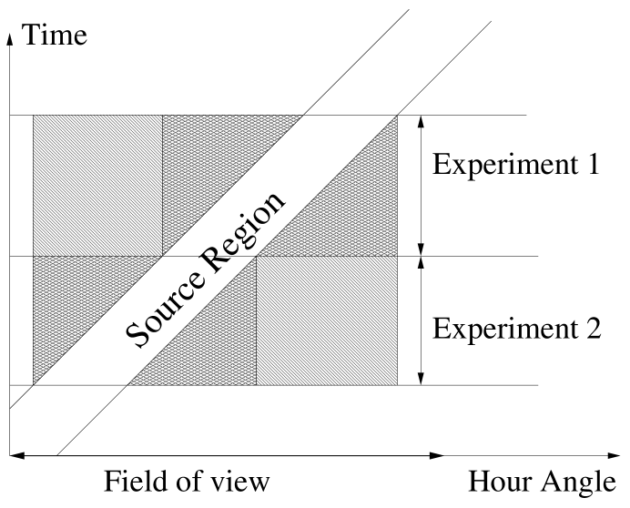
Figure 2: Illustration of difference between union and compounding of experiments.

However, the two experiments can be combined in a different way, if the stability assumption (1) is common for both observations, namely, the two data sets can be united and the time swapping procedure can be applied to this common data set. Such a compounding may lead to increased total significance if otherwise useless information obtained during experiment 1 can prove to be valuable for experiment 2 and vise versa. The situation is illustrated on the figure 2 where two contiguous experiments are presented. The shaded area is the united off-source region, whereas, the heavily shaded is the combination of the independently useful off-source regions of the two experiments. It is seen that in united data set $N_{s}^{(union)}\equiv N_{s}^{(1)}+N_{s}^{(2)}$, $N_{b}^{(union)}\simeq N_{b}^{(1)}+N_{b}^{(2)}$ (statistically equal), but $\alpha^{(union)}\leq\alpha^{(1,2)}$ because $\alpha$’s are ratios of exposures of on- and off-source regions, the latter one being expanded by the unification. Therefore, significance

$$S_{union}=\frac{N_{s}^{(union)}-N_{b}^{(union)}}{\sqrt{N_{s}^{(union)}+\alpha^{(union)}N_{b}^{(union)}}}$$

is statistically higher than $S_{compound}$ because of its lower denominator. The increased sensitivity provides an incentive to broaden the limits of integration (2) for as long as stability assumption (1) allows.

5 Detector Stability Assumption Test. Diurnal Modulations.

Despite the fact that no reconfigurations to the detector on the short time scale are made, the acceptance of the array $G(x)$ depends on transmission properties of the atmosphere and therefore, verification of the stability assumption (1) is still warranted [53].

The test of stability would be a comparison of two acceptances $G_{1}(x)$ and $G_{2}(x)$ measured at different times $t_{1}$ and $t_{2}$. On physical grounds, the detector possesses a certain degree of azimuthal symmetry, so does the atmosphere, therefore acceptance is considered as function of zenith and azimuth angles $G(z,A)$. A measurement is a generation of histograms $G_{1}(z,A)$ and $G_{2}(z,A)$ from the data for a certain duration of time around $t_{1}$ and $t_{2}$. (This interval was chosen to be 30 solar minutes.) These histograms are then to be compared using a significance test. It has to be recognized that presence of sources on the sky will mimic instability (section 7), therefore, zenith and azimuth angle distributions alone are compared instead. The test is based on ideas of compounding probabilities from independent significance tests [54] and is implemented as a series of $\chi^{2}$ tests of $G_{i}(x)$ and $G_{j}(x)$ (yielding $\chi^{2}(t_{i},t_{j})$) and then combined $\chi^{2}_{total}(\Delta t)$ for time separation $\Delta t=t_{i}-t_{j}$ is calculated:

$$\chi^{2}_{total}(\Delta t)=\sum_{\Delta t=t_{i}-t_{j}}\chi^{2}(t_{i},t_{j})$$

Figure 3: Results of stability test on data collected between July 19, 2000 and September 17, 2000 are presented. Horizontal axis is time separation $\Delta t$ in 30 minute units, vertical axis is corresponding $\frac{\chi^{2}_{total}(\Delta t)}{m_{total}(\Delta t)}$. Top plots are the test of zenith distributions, middle and bottom ones are the test of azimuth distributions for $0^{\circ}<z<30^{\circ}$ and $30^{\circ}<z<50^{\circ}$ respectively. On the left all data were used, on the right, only events passing $X_{2}>2.5$ cut. Solid horizontal line is the expected value of one if the stability assumption holds.

The test statistic $\chi^{2}_{total}(\Delta t)$ so obtained follows a $\chi^{2}$ distribution with $m_{total}=\sum_{\Delta t=t_{i}-t_{j}}m(t_{i},t_{j})$ degrees of freedom if observed differences are of random nature only. The average of $\chi^{2}_{total}$ is equal to $m_{total}$ while its variance is equal to $2m_{total}$. The results of such a test are presented on figure 3 as the plot of $\frac{\chi^{2}_{total}(\Delta t)}{m_{total}(\Delta t)}$. The closer the plotted value to the expected one, the better the assumption of stability (1) holds. It is seen from the plots that the degree of violation of the assumption grows with time separation $\Delta t$ as might be expected, but then it drops before growing again. This is interpreted as presence of a periodic component which insured that two acceptances $G_{1}(z)$ and $G_{2}(z)$ separated by 24 solar hours are “closer” to each other than, say, those separated by only 12. Azimuthal distributions show violation of the stability assumption to a lesser degree. This statement is considered to be true after application of the hadron rejection cut as well. Thus, despite the fact that no human intervention on the short time scale is made, the acceptance of the detector changes. As was seen in section 4, the duration of the validity of the assumption (1) defines the time integration limits in equation (2) which, in turn, defines the off-source region. Inasmuch as search for very weak signal requires sensitivity pushed to its limits, care is taken to improve the stability assumption in particular with regard to zenith angle dependence.

The investigation of changes in zenith distribution (simplified by the above noted periodicity) was performed in the following way [55]. Every half hour, a zenith distribution is generated from registered events. These distributions are compared to the average distribution accumulated over a one day period. Half hour distributions and the average one are normalized and then subtracted to give a plot of distribution’s shape change. It was observed that the shape of this change is approximately constant with amplitude varying from half hour to half hour. Therefore, the improved stability assumption is chosen to be of the form:

$$N(x,t)=G(x)R(t)e^{\theta(t)K(z)+q(\theta(t))}\;dt$$ (6)

where $\theta(t)$ is the amplitude of the correction at time $t$, $K(z)$ is the polynomial correction function coefficients of which are obtained from the above study (see appendix 14), $q(\theta(t))$ is the normalization factor so that $\int G(x)e^{\theta(t)K(z)+q(\theta(t))}dx=1$.

The choice (6) of the form of time dependence of a distribution is motivated by the Darmois theorem [56]. According to this theorem, exponential class (6) of probability density functions is the only class which admits number of sufficient statistics for unknown parameter $\theta$ independent of the number of observations. In particular, if $(Z_{1},Z_{2},...,Z_{N})$ is a random sample of size $N$ from the distribution (6), then

$$Y=\sum^{N}_{i=1}K(Z_{i})$$

is sufficient statistics for $\theta$. The importance of sufficiency is explained by the fact that $Y$ exhausts all the information about $\theta$ that is contained in the sample.

By differentiating

$$\int G(z)e^{\theta K(z)+q(\theta)}dz=1$$

twice with respect to $\theta$ we obtain the following two relations for expectation and variance:

$$E[K(Z)]=-q\prime(\theta)$$

$$var[K(Z)]=-q\prime\prime(\theta)$$

Both of these properties allow estimating parameter $\theta$ from the data. Indeed, because $\theta=0$ corresponds $q=0$ (no correction to average distribution), both $\theta$ and $q$ can be determined as

$$\left\{\begin{array}[]{rcl}\theta&=&2\frac{q\prime(\theta)-q\prime(0)}{q\prime\prime(\theta)+q\prime\prime(0)}+O(\theta^{2})\\ q(\theta)&=&\frac{1}{2}(q\prime(\theta)+q\prime(0))\theta+O(\theta^{2})\end{array}\right.$$

Expectation and variance and therefore $q\prime$ and $q\prime\prime$ are determined from the sample and thus are known. The example of the average daily amplitude dependence is shown on figure 4. The value of the amplitude is typically within $\pm 4\cdot 10^{-5}$ range. The plot can also be used to justify the choice of half hour intervals for the amplitude measurement. (This, however, is already seen from the figure 3.)

Figure 4: Average daily dependence of the zenith correction amplitude $\theta$ derived from July 19 - September 17, 2000 Milagro data after application of the hadron rejection cut.

6 Accounting for Modulations in the Framework of Time Swapping Method.

Incorporation of the improved stability assumption (6) into the framework of time swapping is equivalent to modification of Monte Carlo integration where generated events are distributed according to $G(x)R(t)e^{\theta(t)K(z)+q(\theta(t))}$ instead of $G(x)R(t)$. This is accomplished by means of the rejection method [52]. In this method, an event is drawn from the $G(x)R(t)$ distribution as before. But now, the candidate event time is accepted only if a random variable $p$ distributed uniformly between 0 and $P(z)=\max_{\{t\}}e^{\theta(t)K(z)+q(\theta(t))}$ is such that $p<e^{\theta(t)K(z)+q(\theta(t))}$. (Parameters $\theta$ and $q(\theta)$ are assumed to be known at this stage.) If this inequality is violated, another candidate time is sought and then tried. This is continued until time is accepted, resulting in generation of event. Inasmuch as generation of the events is based on the improved stability assumption, the rest of the data analysis algorithm is preserved.

(a) Distribution of $\chi^{2}$ for 90 bin histogram. Solid line is the best fit of $\chi^{2}$ distribution function with 84.11 degrees of freedom.

(b) Distribution of $\chi^{2}$ for 360 bin histogram. Solid line is the best fit of $\chi^{2}$ distribution function with 337.0 degrees of freedom.

Figure 5: Plots showing Monte Carlo simulated distributions of $\chi^{2}$ of the difference of histograms with 90 and 360 bins. Both histograms have the same number of entries (5713).

(a) Distribution of $\chi^{2}$ for standard stability assumption (equation 1). Solid line is the best fit of $\chi^{2}$ distribution function with 93.84 degrees of freedom. The goodness of this fit is characterized by $\chi^{2}/ndf=506.2/50$.

(b) Distribution of $\chi^{2}$ for improved stability assumption (equation 6). Solid line is the best fit of $\chi^{2}$ distribution function with 84.10 degrees of freedom. The goodness of this fit is characterized by $\chi^{2}/ndf=91.34/86$.

Figure 6: Plots showing distributions of $\chi^{2}$ of the difference of simulated and real zenith angle distributions for every half hour with and without correction. The expected number of degrees of freedom is 84.25. Both histograms have the same number of entries (2073).

(a) Distribution of $\chi^{2}$ for standard stability assumption (equation 1). Solid line is the best fit of $\chi^{2}$ distribution function with 339.6 degrees of freedom. The goodness of this fit is characterized by $\chi^{2}/ndf=69.82/83$.

(b) Distribution of $\chi^{2}$ for improved stability assumption (equation 6). Solid line is the best fit of $\chi^{2}$ distribution function with 337.6 degrees of freedom. The goodness of this fit is characterized by $\chi^{2}/ndf=92.33/92$.

Figure 7: Plots showing distributions of $\chi^{2}$ of the difference of simulated and real azimuth angle distributions for every half hour with and without correction. The expected number of degrees of freedom is 337.5. Both histograms have the same number of entries (2073).

In order to illustrate how well the correction works real and generated distributions are compared using a $\chi^{2}$ test. The zenith angle distribution is split into 90 bins, and azimuth one into 360. A word of precaution is appropriate: the real and generated distributions are not independent, one is produced from the other using swapping technique. Due to implementation of the time swapping method (8 hour integration time window) and because distributions are accumulated every 30 minutes, the number of degrees of freedom in the $\chi^{2}$ test should be lower than one would expect from the usual histogram bin considerations by 1 for every 16 bins or 84.25 and 337.5 for 90 and 360 bin histograms respectively. This is supported by Monte Carlo simulations presented on figure (5) where the values of $\chi^{2}$ resulted from the test are histogramed.

Figure (6) demonstrates zenith angle distribution comparisons with and without the correction. From these plots it is clearly seen how a bias of the standard method is removed. A similar study was carried out for azimuth angle distribution. Figure (7) demonstrates the results of the study and shows that azimuth variation, if any, is on a much smaller scale than the zenith one. Note, that no azimuthal correction was applied, therefore, a slight change in the azimuth distribution test is due to possible correlation between zenith and azimuth angles of the detected events. Thus, the improved stability assumption (equation 6) is considered to be valid for the 8 hour duration of timing integration.

7 Known Anisotropies.

It was, so far, conceded that no anisotropy on the sky is present. This, together with the stability assumption had lead to the equation (1). In fact, if there are known sources on the sky, then the number of registered events is given by:

$$dN(x,t)=S(x,t)\cdot G(x)\cdot R(t)\;dxdt$$

where $S(x,t)$ describes the strength of the sources as function of local coordinates and time. (This is how anisotropy can mimic detector instability.)

There are two known sources, actually sinks, on the sky: the Sun and the Moon [57]. Because the anisotropy function $S(x,t)$ produced by them is not known, the anisotropy is handled by vetoing the $\pm 5^{\circ}$ degree regions around the objects. This entails treating them as part of the source bin during Monte Carlo integration and disregarding generated events in the background estimation $N_{b}$ if they fall within the veto region. In general, known small scale anisotropies must be vetoed as described, known large scale ones have to be incorporated into the stability assumption. These become part of the null hypothesis.

Chapter 9 Alternative Hypothesis.

The construction of the alternative hypothesis, or more precisely, of critical regions is based on the knowledge about the Galactic gamma ray emission available to date [9, 7]. Among all experiments operated at different energies the EGRET telescope is the one of closest energy range to Milagro and made a convincing detection of emission. The data made available by the EGRET collaboration [59, 7] is the foundation of the alternative hypothesis. Because of the change of the primary emission mechanism between MeV and GeV energy regions from bremsstrahlung to $\pi^{0}$ decay [14], only highest EGRET energy data points are used in the formulation. Figure 1(a) plots the longitude dependence of the EGRET emission flux in the $\pm 2^{\circ}$ latitude band along the Galactic equator at energies 10-30 GeV. Figure 1(b) shows the Milagro Galactic disk exposure as a function of Galactic longitude. The expected significance which is roughly proportional (equation (1)) to the product of the signal flux and the square root of the exposure is presented on figure 1(c).

Thus, the region of Galactic disk with $l\in(20^{\circ},100^{\circ})$ is the region where highest significance is expected provided the emission model of EGRET is valid at TeV energies. Therefore, the region of $l\in(20^{\circ},100^{\circ})$ is selected as Milagro inner Galaxy. Due to the fact that the inverse Compton mechanisms may result in a wider latitude distribution than that of the gas column density, the region with $|b|<5^{\circ}$ is also considered. The two regions with $l\in(140^{\circ},220^{\circ})$, $|b|<2^{\circ}$ and $|b|<5^{\circ}$ are also selected as Milagro outer Galaxy. These parts of the disk are selected due to their high exposure. These regions are analyzed separately, however $|b|<2^{\circ}$ and $|b|<5^{\circ}$ ones are not independent for the same longitude range. The regions were selected before the analysis was performed.

(a) Total flux at 10-30 GeV in $|b|<2^{\circ}$ disk.

(b) Milagro exposure of $|b|<2^{\circ}$ disk.

(c) The expected relative significance.

Figure 1: Plots showing the construction of the critical region for the alternative hypothesis based on the EGRET data.

Chapter 10 Results.

1 Results of the Measurements.

The results presented below are obtained after the analysis of data collected between July 19, 2000 and September 10, 2001 by the Milagro detector. The starting date corresponds to the commissioning of the hadron rejection algorithm, the ending date is when the experiment was turned off for a major scheduled maintenance.

To ensure high quality of the data, the periods with abnormal event rate with and without the hadron rejection cut were eliminated from the analysis. These may indicate possible detector problems. Parts of the data were also discarded if the Milagro log-book showed entries of some hardware/software problems or indications of unstable operation. Periods of abnormal zenith angle distribution of events were also discarded. Other cuts applied include $N_{fit}>20$ to ensure good angular resolution and the zenith angle cut $0^{\circ}<z<50^{\circ}$ due to stability considerations (appendix 14).

The null hypothesis tested consists of:

• There is no emission from the Galactic plane except for background.

• All of the detected events are due to background and it is isotropic except for $\pm 5^{\circ}$ region around the Sun and the Moon. (Events from these regions are vetoed.)

• Detected events satisfy the stability equation (6).

• The null hypothesis also includes certain aspects of shower development and detector operation important for the detection and reconstruction of events. These include reconstructions algorithms and detector calibration procedures.

Because the emission from the Galactic plane is under investigation, events arriving from the $\pm 7^{\circ}$ band along the Galactic equator are excluded from the background generation (see section 2). Four regions of the disk (selected a priory) were studied. The Milagro inner Galaxy with Galactic longitude $l\in(20^{\circ},100^{\circ})$, $|b|<2^{\circ}$ and $|b|<5^{\circ}$; and Milagro outer Galaxy with $l\in(140^{\circ},220^{\circ})$, $|b|<2^{\circ}$ and $|b|<5^{\circ}$. The results are given in the table 1.

	Inner Galaxy
	$|b|<2^{\circ}$	$|b|<5^{\circ}$
$N_{s}$	$(43446.6\pm 6.6)\cdot 10^{3}$	$(10823.8\pm 1.0)\cdot 10^{4}$
$N_{b}$	$(43426.7\pm 2.7)\cdot 10^{3}$	$(10819.7\pm 0.5)\cdot 10^{4}$
$N_{\gamma}/N_{b}$	$(+4.57\pm 1.64)\cdot 10^{-4}$	$(+3.77\pm 1.08)\cdot 10^{-4}$
significance	+2.8	+3.5
	Outer Galaxy
	$|b|<2^{\circ}$	$|b|<5^{\circ}$
$N_{s}$	$(46409.1\pm 6.8)\cdot 10^{3}$	$(11588.6\pm 1.1)\cdot 10^{4}$
$N_{b}$	$(46413.0\pm 3.0)\cdot 10^{3}$	$(11590.1\pm 0.6)\cdot 10^{4}$
$N_{\gamma}/N_{b}$	$(-0.82\pm 1.6)\cdot 10^{-4}$	$(-1.28\pm 1.06)\cdot 10^{-4}$
significance	-0.5	-1.2

Table 1: Summary of the results for the analysis of the Milagro inner and outer Galaxy ($N_{\gamma}\equiv N_{s}-N_{b}$).

As seen from the table 1 the results of the analysis for the inner Galaxy indicate violation of the null hypothesis. The null hypothesis is rejected with the significance of 3.5 or the probability that it is rejected by chance fluctuations is only $2.3\cdot 10^{-4}$ (see table 1). A detection of a source is usually claimed if the chance probability is less than 0.1%.

In order to be able to interpret the result as a presence of excess of events in the direction of the Galactic plane, other constituents of the null hypothesis have to be examined. The aspects of detector operation and event reconstruction are unlikely to produce localized structure on the sky, they should rather show up as global changes such as in total event rate, in zenith angle distribution of detected events. These were carefully monitored. A violation of the stability assumption may, however, “produce” large scale structures on the sky (and vise versa).

Isotropy of the background is another ingredient. Because of the random bending of cosmic rays in the galactic magnetic fields which are responsible for the isotropy of the background, small deviations from isotropy are expected to be smooth and therefore reveal themselves as large scale structures too. According to indications in the literature from underground muon experiments [60] a slight anisotropy may be present which is parametrized by the authors as:

$$R(\alpha)=1+r_{0}\cos(\alpha-\alpha_{0})$$

where $r_{0}=(5.6\pm 1.9)\cdot 10^{-4}$, $\alpha_{0}=8.0^{\circ}\pm 19.1^{\circ}$. To study the systematic error caused by a possible neglect of the effect, a computer simulation was employed. In this simulation a data set equivalent to the 18 times the real one was generated. The anisotropy was simulated at the specified level but standard analysis was applied. The results of this simulation are presented in the table 2.

	$|b|<2^{\circ}$	$|b|<5^{\circ}$
Inner Galaxy	$(-3.7\pm 3.8)\cdot 10^{-5}$	$(-4.0\pm 2.5)\cdot 10^{-5}$
Outer Galaxy	$(-5.4\pm 3.7)\cdot 10^{-5}$	$(-1.7\pm 2.4)\cdot 10^{-5}$

Table 2: Results of the systematic error study for $N_{\gamma}/N_{b}$.

Despite the computational error bars that are only about 4.3 times smaller than the ones in the real data (limited by the computer time), this is enough to show that this anisotropy is also unlikely to be responsible for the observed result. It should be noted that the discussed muon anisotropy need not be identical to that of the cosmic ray air showers in the Milagro energy range. However, the result may be interpreted as a systematic correction if the anisotropy is established to exist [61]. Within limits of the calculation, the correction is not inconsistent with being zero.

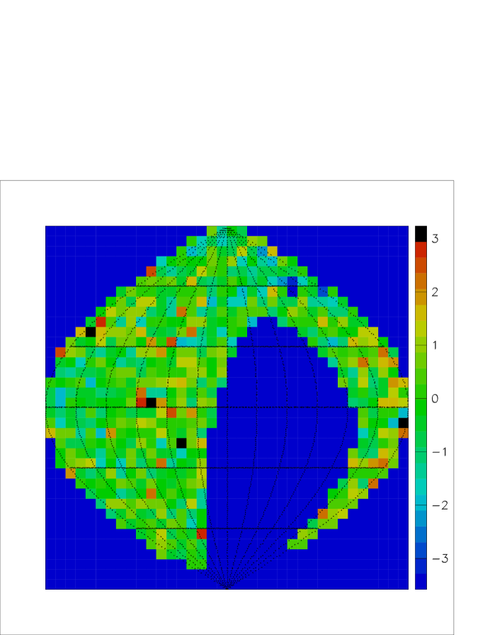
Figure 1: Significance map of the sky in Galactic coordinates. Emission from the inner Galactic region is seen. Grid lines are plotted every $30^{\circ}$ in longitude and latitude. The Galactic center, not visible by Milagro, is in the middle of the map. Galactic longitude increases to the left.

Figure 2: The distribution of significances of individual cells of figure 1. The best fit of a Gaussian distribution is also shown. It agrees well with the standard normal distribution (zero mean and unit variance).

(a) Latitude profile of $N_{\gamma}/N_{b}$ for inner Galaxy. The value of $\chi^{2}$ with respect to 0 is 72.10 with 83 bins.

(b) Latitude profile of $N_{\gamma}/N_{b}$ for outer Galaxy. The value of $\chi^{2}$ with respect to 0 is 116.9 with 84 bins.

Figure 3: Latitude profiles of $N_{\gamma}/N_{b}$ for the inner and outer Galaxy.

In the process of background estimation using the time swapping method, the background was generated and saved for the entire sky, not only for the regions of interest. This may serve to provide additional information.

Figure 1 shows the 2 dimensional map of the significance in the Galactic coordinates with coarse bins appropriate for a large scale structure. An enhancement in the region of inner Galaxy is seen. Another feature visible on the plot is a valley at $l=-150^{\circ}$, $b=+60^{\circ}$. It may be interpreted as an indication of a possible small anisotropy of the cosmic rays. Haverah Park [62] and Yakutsk [63] experiments have found a deficit of flux from the Galactic North in the energy range of $10^{15}-10^{19}$ eV, however, the existence of such an anisotropy in the Milagro energy range is unknown. Figure 2 presents the distribution of significances of individual cells of figure 1. The distribution is expected to be the standard normal one (see discussion following equation (1)) with which it agrees well. Therefore, the observed excesses and deficits are statistically allowed.

A signature of the galactic nature of the emission is presence of a ridge along the galactic equator. Therefore, another check is provided by a lateral distribution plot of $N_{\gamma}/N_{b}$ (figure 3). The plot for the inner Galaxy (figure 3(a)) shows the excess in the region around the equator ($b=0$) as expected and is flat outside suggesting that it is the disk which produces the excess. The plot for the outer Galaxy (figure 3(b)) does not show presence of excess in the plane region, however, indicates a possible existence of a large scale anisotropy. The exact interpretation of the values of $\chi^{2}$ given in the captions to the figures is, however, difficult. Calculation of values and errors for the points plotted outside of the excluded region suffers from the dependence problem such as illustrated on figure 1. Also, the points in adjacent bins are positively correlated, therefore, number of degrees of freedom is effectively lower than what is expected from the number of bins considerations. However, if it is assumed that anisotropy is present and is modeled by a straight line in the inner Galactic region and by a parabola in the outer one, then it is possible to estimate its effect by fitting a straight line in the region of $5^{\circ}<|b|<60^{\circ}$ for the case of the inner Galaxy and quadratic polynomial in the region of $5^{\circ}<|b|<40^{\circ}$ for the case of the outer Galaxy and interpolating it into the plane $|b|<5^{\circ}$. This results in the estimated contribution of $(+0.54\pm 0.34)\cdot 10^{-4}$ (inner Galaxy) and $(-0.48\pm 0.65)\cdot 10^{-4}$ (outer Galaxy) to the measured ratios $N_{\gamma}/N_{cr}$. These values have to be subtracted from the results for the ratios of table 1 as systematic corrections if the anisotropy is known to be of the form discussed [61]. They also are not inconsistent with being zero.

It is therefore concluded that the outer Galaxy does not show excess and the measurements may be used to set upper limits for the emission. The results for the inner Galaxy, if interpreted as gamma ray emission, may be used to calculate the gamma ray flux.

2 Interpretation of the Results.

In what follows it is assumed that the emission from the Galactic plane is known to exist and that the observed excess in the galactic plane is due to gamma rays. With these assumptions in mind, the results of the measurements can be used to establish some properties of the emission.

Assuming simple power law emission spectrum independent of Galactic coordinates for Galactic gamma rays in the Milagro energy range or, equivalently, assuming gamma ray signal function to be in the form of equation (4) and given power law spectrum of cosmic-ray flux at the Earth ($F_{cr}(>1TeV)=1.2\cdot 10^{-5}(cm^{-2}s^{-1}str^{-1})$ [64], $\alpha_{cr}=2.7$) it is possible to use results of the table 1 to relate integral flux of gamma rays above 1 TeV ($F_{\gamma}(>1TeV)$) with their assumed spectral index $\alpha_{\gamma}$ (equation 5). The dimensionless coefficient $\eta(\alpha_{\gamma},\alpha_{cr})$ needed for this conversion is plotted on figure 4 for $\alpha_{cr}=2.7$. The value of this coefficient reflects efficiency of the cosmic ray rejection algorithm and for $\alpha_{\gamma}=\alpha_{cr}$ has a direct interpretation of a ratio of effective areas after the cut. The integral flux of gamma rays above 1 TeV obtained is plotted on figure 5 as solid lines.

Figure 4: Dimensionless coefficient $\eta(\alpha_{\gamma},\alpha_{cr})$ plotted as function of $\alpha_{\gamma}$ ($\alpha_{cr}=2.7)$ for the inner Galaxy with $|b|<5^{\circ}$. Other regions of the Galaxy considered have very similar exposure and therefore the presented coefficient is almost identical.

	$|b|<2^{\circ}$	$|b|<5^{\circ}$
Inner Galaxy	$(1.82\pm 0.25)\cdot 10^{-6}$	$(1.18\pm 0.14)\cdot 10^{-6}$
Outer Galaxy	$(1.90\pm 0.81)\cdot 10^{-7}$	$(3.45\pm 0.60)\cdot 10^{-7}$

Table 3: Average integral flux of photons ($cm^{-2}sr^{-1}s^{-1}$) in the 10-30 GeV energy range measured by EGRET in the corresponding regions of the Galactic plane. Isotropic diffuse component has been subtracted [7, 59].

(a) Inner Galaxy, $|b|<2^{\circ}$.

(b) Inner Galaxy, $|b|<5^{\circ}$.

(c) Outer Galaxy, $|b|<2^{\circ}$.

(d) Outer Galaxy, $|b|<5^{\circ}$.

Figure 5: Integral flux of photons in different parts of Galactic disk with energies above 1 TeV or corresponding 99.9% upper limit for assumed differential spectral index $\alpha_{\gamma}$ are shown as solid lines. The dashed lines represent the extrapolated EGRET measurements in the 10-30 GeV energy range and the same filed of Galaxy. The error corridors are shown as lines with dots.

On the other hand, given the measurements of EGRET (table 3) and assuming that power law index $\alpha_{\gamma}$ is constant above 10 GeV it is possible to extrapolate the EGRET measurement in the highest energy bin 10-30 GeV to the 1 TeV region. This is shown on figure 5 as dashed lines. Both EGRET and Milagro measurements are presented together with the corresponding error corridors. The intersection of the corridors provides the spectral index and integral flux that is consistent with the EGRET and Milagro data. In the case of Milagro upper limit, the limit itself is presented. This comparison leads to estimation of the spectral index $\alpha_{\gamma}=2.59\pm 0.07$ and flux $F(>1TeV)=(9.5\pm 2.0)\cdot 10^{-10}\;cm^{-1}\;sr^{-1}\;s^{-1}$ in the region of inner Galaxy and to a lower limit of $\alpha_{\gamma}>2.49$ and flux $F(>1TeV)<4.5\cdot 10^{-10}\;cm^{-1}\;sr^{-1}\;s^{-1}$ in the outer Galaxy. (Regions with $|b|<5^{\circ}$ are used for final calculations because of greater sensitivity of Milagro.) These findings may be used to exclude models which predict a strong enhancement of the diffuse flux compared to conventional mechanisms. Model predictions attempting to explain the excess flux in the GeV region measured by EGRET by assuming an increased inverse Compton component [13] or by harder proton spectrum [1] or by considering contribution from unresolved supernova remnants [2] are given in literature for different ranges in Galactic latitude and longitude and can not be directly compared with the presented results. However, it is possible to find spectral indexes in the energy range above 1 GeV as measured by EGRET averaged over the Milagro inner and outer Galaxies (table 4) and compare them with the above results. While the EGRET spectral index does not contradict to the Milagro upper limit for the region of outer Galaxy, measurements of the index in the inner Galaxy exclude the possibility of constant spectral index and require softening of the spectrum between EGRET and Milagro energy regions. This is also illustrated on figures 6 for the regions of inner and outer Galaxy with $|b|<5^{\circ}$.

	$|b|<2^{\circ}$	$|b|<5^{\circ}$
Inner Galaxy	$2.346\pm 0.028$	$2.365\pm 0.016$
Outer Galaxy	$2.560\pm 0.054$	$2.487\pm 0.059$

Table 4: Spectral index $\alpha_{\gamma}$ derived from the EGRET data in the 1-30 GeV energy range in the corresponding regions of the Galactic plane. (The data was made available by [59].)

(a) Inner Galaxy.

(b) Outer Galaxy.

Figure 6: Integral flux of photons from $|b|<5^{\circ}$ region multiplied by photon energy $E$ is plotted. EGRET data points in the energy range of 1-30 GeV are also shown. The dashed line is the spectrum derived from the EGRET data above 1 GeV.

Chapter 11 Conclusions.

A search for diffuse gamma ray emission from the Galactic plane has been performed using data collected by the Milagro detector between July 19, 2000 and September 10, 2001. Four regions of the disk were studied. An excess has been observed from the regions of the Milagro inner Galaxy defined by $l\in(20^{\circ},100^{\circ})$, $|b|<2^{\circ}$ and $|b|<5^{\circ}$ with the significance of $2.6\cdot 10^{-3}$ and $2.3\cdot 10^{-4}$ respectively. The emission from the region of the Milagro outer Galaxy defined by $l\in(140^{\circ},220^{\circ})$, $|b|<2^{\circ}$ and $|b|<5^{\circ}$ is not inconsistent with being that of background only.

The results are interpreted assuming a simple power law energy spectrum. Given the EGRET measurements, the integral gamma ray flux with energies above 1 TeV has been obtained, yielding $F(>1TeV)=(9.5\pm 2.0)\cdot 10^{-10}\;cm^{-1}\;sr^{-1}\;s^{-1}$ with spectral index $\alpha_{\gamma}=2.59\pm 0.07$ for the region of inner Galaxy. The 99.9% upper limit for the diffuse emission in the region of outer Galaxy is set at $F(>1TeV)<4.5\cdot 10^{-10}\;cm^{-1}\;sr^{-1}\;s^{-1}$ assuming a differential spectral index of $\alpha_{\gamma}=2.49$. These observations are compatible with earlier upper limits obtained by the Whipple observatory at 500 GeV [8]. The upper limit for the outer Galaxy is also consistent with the extrapolation of EGRET measurements between 1 and 30 GeV. Extrapolation of the EGRET measurements between 1 and 30 GeV for the region of inner Galaxy using constant power law spectral index is incompatible with the Milagro data. This indicates softening of the spectrum at energy between 10 GeV and 1 TeV. These observations may be used to constrain models of Galactic emission [1, 2, 13].

During preparation of this manuscript, the Milagro detector continued to operate and collected more data. The analysis of these data will confirm or refute the observations. Regardless of the outcome, the combined data set will provide for more sensitive measurement of the diffuse gamma ray emission at energies near 1 Tev. The Milagro detector is being continuously upgraded both on software and hardware level. New event reconstruction algorithms may become available in the near future. These, however, will have no affect on the data collected so far. In terms of hardware, Milagro is being supplimented by an outrigger array, which will enable better hadron rejection as well as energy determination and angular resolution. As more and better quality data become available, it will be possible to study the question of cosmic ray anisotropy extensively using the Milagro data itself. This presents an interest not only in the context of the search for the Galactic gamma ray emission, but is valuable by itself as the detection of Compton-Getting effect may become possible [65].

Chapter 12 Arguments pertaining to equation 1.

The Poisson distribution of an integer random variable $n$ is given by:

$$P_{\mu}(n)=\frac{\mu^{n}}{n!}e^{-\mu}$$

where $\mu$ is a parameter of distribution. One can show that both average and dispersion of $n$ are equal to $\mu$. It is intended to show that for large $\mu$, the Poisson distribution approaches Gaussian:

$$G(x)=\frac{1}{\sqrt{2\pi}\sigma}e^{-\frac{(x-x_{0})^{2}}{2\sigma^{2}}}$$

with average $x_{0}=\mu$ and dispersion $\sigma^{2}=\mu$.

For the case of large $\mu$ and $n$ being not too different from it, the Stirling formula for the factorial can be applied:

$$n!\approx\sqrt{2\pi n}\;n^{n}e^{-n}$$

with relative error of order of $(e^{\frac{1}{12n}}-1)$, leading to

$$P_{\mu}(n)\approx\frac{e^{n-\mu}}{\sqrt{2\pi n}}\;\left(\frac{\mu}{n}\right)^{n}=e^{y(n)}$$

The exponent $y(n)$ can be expanded in Taylor series around $\mu$:

$y(\mu)$	=	$-\ln\sqrt{2\pi\mu}$
$y^{\prime}(\mu)$	=	$-\frac{1}{2\mu}$
$y^{\prime\prime}(\mu)$	=	$-\frac{1}{\mu}\left(1+\frac{1}{2\mu}\right)$
$y^{\prime\prime\prime}(\mu)$	=	$+\frac{1}{\mu^{2}}\left(1-\frac{1}{\mu}\right)$
$y^{(4)}(\mu)$	=	$-\frac{2}{\mu^{3}}\left(1-\frac{3}{2\mu}\right)$

$$y(n)=-\ln\sqrt{2\pi\mu}-\frac{1}{2\mu}(n-\mu)-\frac{1}{2\mu}\left(1+\frac{1}{2\mu}\right)(n-\mu)^{2}+$$

$$+\frac{1}{6\mu^{2}}\left(1-\frac{1}{\mu}\right)(n-\mu)^{3}+\cdots+O\left(\frac{(n-\mu)^{k}}{\mu^{k-1}}\right)$$

In this Taylor series (recalling that $\mu$ is large) the second term can be neglected compared to the leading if $|n-\mu|\ll 2\mu\ln\sqrt{2\pi\mu}$, third if $|n-\mu|\ll\sqrt{2\mu\ln\sqrt{2\pi\mu}}$, fourth if $|n-\mu|\ll(6\mu^{2}\ln\sqrt{2\pi\mu})^{1/3}$, all higher terms if $|n-\mu|\ll(\mu^{k-1}\ln\sqrt{2\pi\mu})^{1/k}$. It is seen that the first condition is least restrictive one, second, however, is the most limiting. Thus, keeping only two leading terms in $|n-\mu|$ will result:

$$y(n)\approx-\ln\sqrt{2\pi\mu}-\frac{1}{2\mu}\left(1+\frac{1}{2\mu}\right)(n-\mu)^{2}$$

with restriction $|n-\mu|\ll(6\mu^{2}\ln\sqrt{2\pi\mu})^{1/3}$. This means that $n$ has to be not too far off $\mu$ and when $\mu$ is large the use of the Sterling formula is justified. The Poisson distribution is approximated by Gaussian in the central region:

$$P_{\mu}(n)=\frac{\mu^{n}}{n!}e^{-\mu}\approx\frac{1}{\sqrt{2\pi\mu}}e^{-\frac{(n-\mu)^{2}}{2\mu}},\;\;\;|n-\mu|\ll(6\mu^{2}\ln\sqrt{2\pi\mu})^{1/3},\;\;\;\mu\gg 3/2$$

Examining the equation 1 if null hypothesis is true, it follows from the above, that the numerator is distributed under the Gauss law with zero mean if both $N_{1}$ and $N_{2}$ are large and are not too different from $\mu_{1,2}=\lambda t_{1,2}$. By construction, if null hypothesis is true and $N_{1,2}\sim\mu_{1,2}$, the dispersion of $S$ is approximately unity, therefore, the statistic $S$ has normal distribution in $-S_{0}<S<S_{0}$ region around zero. The bound $S_{0}$ is defined by the smallest of the $N$’s and is on the order of

$$S_{0}\ll\left(6N^{1/2}\ln\sqrt{2\pi N}\right)^{1/3}$$ (1)

A Monte Carlo simulation helps to verify the statement. Figure 1 shows the results of such a simulation.

(a) Null hypothesis with parameters $\mu_{2}=5000$, $\mu_{1}=\alpha\mu_{2}$, $\alpha=0.1$ was used. According to equation (1), $S_{0}\ll 8$.

(b) Null hypothesis with parameters $\mu_{2}=15\cdot 10^{6}$, $\mu_{1}=\alpha\mu_{2}$, $\alpha=0.1$ was used. According to equation (1), $S_{0}\ll 39$.

Figure 1: Distributions of statistic $S$ (equation 1) obtained in two runs of Monte Carlo simulations. Best fit to Gauss distribution is made, parameters of the fit are presented. The two curves should agree in the $S_{0}$-neighborhood around zero. Number of entries in each run (about $10^{9}$) was chosen to provide reasonable accuracy in the region plotted.

Chapter 13 Solution of Background Equations.

The problem of exclusion of the source region from the background estimation had led to the problem of solution of the integral equations:

$$\left\{\begin{array}[]{lcl}N_{out}(x)&=&G(x)\int\phi(x,t^{\prime})\cdot R(t^{\prime})\;dt^{\prime}\\ R_{out}(t)&=&R(t)\int\phi(x^{\prime},t)\cdot G(x^{\prime})\;dx^{\prime}\end{array}\right|$$

with respect to $G(x)$ and $R(t)$. $N_{out}(x)$ and $R_{out}(t)$ represent the input data collected from the off-source region, $\phi(x,t)$ is the function which defines its bounds: it is one if $(x,t)$ points into the off-source region and zero otherwise. It is first noted that both $G(x)$ and $R(t)$ enter into equations only as a product $G(x)\cdot R(t)$, therefore, normalization of either of them does not make any difference as long as the product is preserved. Also, if there is a point $x_{0}$ in the local coordinates which is never exposed into the off-source region, that is $\phi(x_{0},t)=0,\;\forall t$, then $N_{out}(x_{0})=0$ and the first equation becomes:

$$0=G(x_{0})\cdot 0$$

leading to $G(x_{0})$ being undefined. Such regions, if any, are marked with a negative value, on-source events with local coordinates from these regions are discarded as having no corresponding background estimate. In such cases, measurement is impossible within the environs of assumptions.

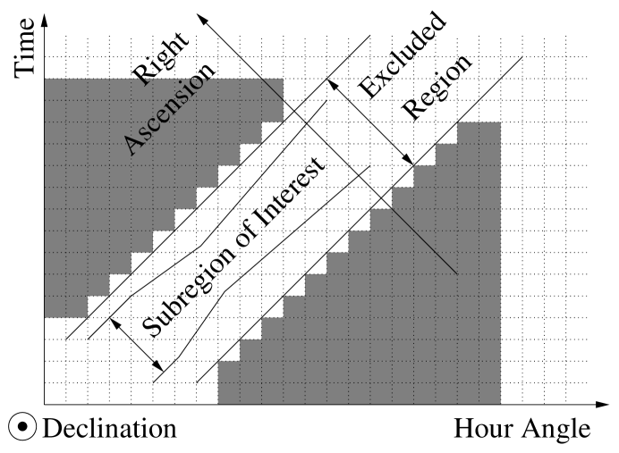
Figure 1: To the formulation of backgroud equations.

Figure 2: To the derivation of recursion relations.

The system of equations is solved numerically. The equations are discretized on a fine grid corresponding to $0.1^{\circ}$ in $x$ and $t$, the integrals become sums, $x$ and $t$ become indexes. Since most often one is interested in celestial objects, the off-source region is defined in declination and right ascension $(\delta,\alpha)$ and due to discretization presents the bound indexes $\alpha_{1}$ and $\alpha_{2}$, $\alpha_{1}<\alpha_{2}$ for every declination index $\delta$. Therefore, for this problem, it is natural to consider local coordinates $x$ as declination and hour angle $(\delta,h)$ rather than zenith and azimuth. The situation is illustrated on figure 1. The shaded area is the off-source region bounded by $\phi(x,t)$ in its discrete form. The region of interest, the on-source region, is defined by some other conditions which are irrelevant for the background equations as long as both regions do not overlap.

Thus, the excluded region, defined by interval $(\alpha_{1},\alpha_{2})$ is translated to local coordinates $h$ and $t$ as region inside intervals $(h_{1},h_{2})$ and $(t_{1},t_{2})$, where

$$\begin{array}[]{l}\left\{\begin{array}[]{lcl}h_{1}&=&t-\alpha_{2}\;\bmod 360^{\circ}\\ h_{2}&=&h_{1}+\alpha_{2}-\alpha_{1}\end{array}\right.\\ \\ \left\{\begin{array}[]{lcl}t_{1}&=&h+\alpha_{2}\;\bmod 24\;hours\\ t_{2}&=&t_{1}+\alpha_{2}-\alpha_{1}\end{array}\right.\end{array}$$

Because of these relations it is convenient to quantize all quantities in the same fashion. This, however, is not required. Here, it is adopted that $\alpha_{1}$ is the index of the first excluded bin, $\alpha_{2}$ is the index of the last excluded bin. So will be $h_{1},t_{1}$ and $h_{2},t_{2}$. The integration is performed using recursion formulas which are illustrated on the $\rho(t)=\int\phi(h^{\prime},t)G(h^{\prime})dh^{\prime}$ example. After integral is replaced by sum, it becomes:

$$\rho(t)=\sum_{h=0}^{h_{1}-1}G(h)+\sum_{h=h_{2}+1}^{N-1}G(h)$$

where $N$ is the number of cells from $0$ to $N-1$ created by the discretization of the hour angle between $0^{\circ}$ and $360^{\circ}$. The limits of the summation are included, that is

$$\sum_{h=a}^{b}G(h)=G(a)+G(a+1)+\cdots+G(b-1)+G(b)$$

Then, it is seen (figure 2) that the integral at some other time $t^{\prime}$ is given by

$$\rho(t^{\prime})=\sum_{h=0}^{h_{1}^{\prime}-1}G(h)+\sum_{h=h_{2}^{\prime}+1}^{N-1}G(h)=\rho(t)+\Delta_{1}-\Delta_{2}$$

where

$$\begin{array}[]{l}\left\{\begin{array}[]{lr}\Delta_{1}=+\sum_{h_{1}}^{h_{1}^{\prime}-1}G(h),&h_{1}^{\prime}>h_{1}\\ \Delta_{1}=-\sum_{h_{1}^{\prime}}^{h_{1}-1}G(h),&h_{1}^{\prime}<h_{1}\\ \Delta_{1}=0,&h_{1}^{\prime}=h_{1}\end{array}\right.\\ \\ \left\{\begin{array}[]{lr}\Delta_{2}=+\sum_{h_{2}+1}^{h_{2}^{\prime}}G(h),&h_{2}^{\prime}>h_{2}\\ \Delta_{2}=-\sum_{h_{2}^{\prime}+1}^{h_{2}}G(h),&h_{2}^{\prime}<h_{2}\\ \Delta_{2}=0,&h_{2}^{\prime}=h_{2}\end{array}\right.\end{array}$$

This scheme is applied for every declination. Integration over time is performed in the similar fashion. It is important to note, that case of $\alpha_{1}=\alpha_{2}$ corresponds to exclusion of one bin. Absence of excluded region for a declination is encoded as $\alpha_{2}=\alpha_{1}-1$, which is the only case with $\alpha_{2}<\alpha_{1}$ allowed. The system is solved by iterations where $R_{out}(t)$ is used as first approximation to $R(t)$. Then, the first equation is solved with respect to $G(x)$ which is used in the second equation to update $R(t)$. The process continues until desired accuracy is reached. In practice, 13-digit precision is achieved after about 15 iterations.

Chapter 14 Zenith Correction.

$$\begin{array}[]{|c|c|c|c|c|c|c|}\hline\cr Period&a&b&c&d&e&A\\ (MJD)&(10^{-6})&(10^{-3})&(10^{-4})&(10^{-1})&(10^{-2})&(10^{0})\\ \hline\cr 1745&&&&&&\\ \updownarrow&+203.0670&-174.6125&+10721.45&-16.27103&-5.631589&-122.02\\ 1813&&&&&&\\ \updownarrow&-27.00866&-19.20310&+291.3698&+4.232470&-129.1226&-698.0\\ 1876&&&&&&\\ \updownarrow&+56.50721&-32.53573&+1355.857&+1.621818&-108.8645&-551.0\\ 1937&&&&&&\\ \updownarrow&+124.5009&-12.71605&+171.8406&+3.488231&-116.1735&-1300.0\\ 2000&&&&&&\\ \updownarrow&-4.604483&-10.42552&+4.944296&+4.006497&-121.4843&-1260.0\\ 2069&&&&&&\\ \updownarrow&-32.60869&-8.961481&-297.4525&+5.175355&-133.4420&-1100.0\\ 2117&&&&&&\\ \updownarrow&-27.23581&-11.71815&+27.33091&+4.266234&-126.5341&-1110.0\\ 2163&&&&&&\\ \hline\cr\end{array}$$

Table 1: Coefficients of the zenith correction function $\Delta(z)$ derived for data which passes the hadron rejection cut $X_{2}>2.5$. MJD, the Modified Julian Day, identifies the validity time period. For instance, MJD 1745 corresponds to July 19, 2000; MJD 2163 corresponds to September 10, 2001 [58].

Figure 1: Correction function $\Delta(z)$. Coefficients corresponding to period MJD 1745 - MJD 1813 were used.

The zenith correction function $\Delta(z)$ describes deviation of the current shape of the zenith distribution from the average one over the same UT day. It is obtained in the iteration process in the form of polynomial of 5-th degree starting with some zero-th approximation. The differences between the two normalized histograms are accumulated according to the sign of amplitude $\theta$ of the fit of a difference into $\theta\Delta(z)$. When all differences according to their corresponding sing of amplitudes are accrued, coefficients of the $\Delta(z)$ are adjusted to provide the best fit. This is the updated function $\Delta(z)$. The procedure is repeated until coefficients of the polynomial stop changing. Then, $\Delta(z)$ is rescaled so that its maximum is equal to one. This is the final form of $\Delta(z)$. The $K(z)$ function is obtained from the $\Delta(z)$ by

$$K(z)=\frac{\Delta(z)}{G(z)}$$

where $G(z)$ is the average zenith distribution. Coefficients of the correction function $\Delta(z)$ are given in the table 1 with its shape defined by:

$$\Delta(z)=A(y^{5}+ey^{4}+dy^{3}+cy^{2}+by+a)$$

where $y=z/90$, $0^{\circ}<z<50^{\circ}$.

The example of the $\Delta(z)$ curve is presented on figure 1 The field of view of the detector was artificially made limited to $0^{\circ}<z<50^{\circ}$ because zenith angle distribution variations outside of this range could not be characterized by such a simple dependence.

References

- [1] F. A. Aharonian and A. M. Atoyan, astro-ph/0009009, 2000.
- [2] E. G. Berezhko and H. J. Völk, Astrophysical Journal, 540, 923-929, 2000.
- [3] A. Borione et al., Astrophysical Journal, 493, 175, 1998.
- [4] P. Chardonnet et al., Astrophysical Journal, 454, 774, 1995.
- [5] F. Lebrun et al., Astrophysical Journal, 274, 231, 1983.
- [6] R.C. Hartman et al., Astrophysical Journal, 230, 597-606, 1979.
- [7] S. D. Hunter et al., Astrophysical Journal, 481, 205, 1997.
- [8] P. T. Reynolds et al., Astrophysical Journal, 404, 206, 1993.
- [9] R. Ong, Physics Reports, 305, 93, 1998.
- [10] http://cossc.gsfc.nasa.gov/cossc/EGRET.html.
- [11] M. Urban et al., Phys. Lett. B, 293, 149 1992.
- [12] H. Bloemen, Annual Review Astronomy and Astrophysics, 27, 469-516, 1989.
- [13] M. Pohl and J. A. Esposito, Astrophysical Journal, 507, 327, 1998.
- [14] D. L. Bertsch et al., Astrophysical Journal, 416, 587, 1993.
- [15] M.S. Longair, High Energy Astrophysics, vol. 1, Cambridge Unversity Press, 1992.
-
[16]
B. Rossi and K. Greisen, Rev. Mod. Phys., 13, 240 (1941).
B. Rossi, High Energy Particles, Prentice-Hall, Englewood Cliffs, N.J., 1952. -
[17]
B. D’Ettorre Piazzoli and G. Di Sciascio, Astropart. Phys. 2
(1994) 1999; Erratum, 2 (1994) 327.
G. Di Sciascio, B. D’Ettorre Piazzoli and M, Iacovacci, Astropart. Phys. 6 (1997) 313. - [18] see for example Review of Particle Properties, Physical Review D50, 1173, 1994.
- [19] R. Becker-Szendy et al. Nuclear Instruments and Methods, A, 324, 363 (1993).
- [20] T. K. Gaisser, Cosmic Rays and Particle Physics, Cambridge University Press, 1990.
- [21] R.. Atkins et al., Nuclear Instruments and Methods, A449, 478, 2000.
- [22] D. Coyne and M. Schneider, First Results on Milagro Water Attenuation Using Measurements from the Upgraded TUBE, Internal Milagro Memo, August 14, 2002.
- [23] http://ik1au1.fzk.de/heck/corsika/
- [24] http://wwwinfo.cern.ch/asd/geant/index.html
- [25] R. Becker-Szendy et al. Nuclear Instruments and Methods, A, 352, 629 (1995).
- [26] Lazar and Roman Fleysher and Peter Nemethy, with Isabel Leonor, Timing Pedestals, Internal Milagro Memo, July 7, 1997.
- [27] L. Fleysher for the Milagro Collaboration, Proc. 26-th ICRC, Salt Lake City, USA, OG4.4.03, 1999.
- [28] Isabel Leonor, TOT-PE Conversion using Occupancy Method, Internal Milagro Memo, April 22, 1998.
- [29] Lazar Fleysher and Roman Fleysher, Milagro Calibration System, Internal Milagro Manual, June 28, 2000.
- [30] Lazar Fleysher and Roman Fleysher, An Introduction to Random Functions, Internal Milagro Memo, May 7, 1999.
- [31] V. S. Pugachev, Theory of Random Function and its Applications to Control Problems. Oxford; New York; Pergamon, Mass. Addison-Wesley, 1965.
- [32] Lazar Fleysher, Roman Fleysher, Allen Mincer, Peter Nemethy, Slewing Extrapolation, Internal Milagro Memo, April 20, 2000.
- [33] Peter Nemethy, Lazar Fleysher, Roman Fleysher, Time Calibration: stability studies, Internal Milagro Memo, June 5, 2000.
- [34] Gaurang B. Yodh, Event Energy Determination. Internal Milagro Memo, March 14, 2000.
- [35] Joe F. McCullough and Javier Bussonos-Gordo, Tuning the Angle Fitter, Sampling and Curvature Corrections for Milagro. Internal Milagro Memo, April 3, 2000.
- [36] Andy Smith, My Likelihood Fitter. Internal Milagro Memo, July 1997.
- [37] Greg Sullivan and Andy Smith, An off-pond Core Finder. Internal Milagro Memo, July 7, 2000.
- [38] Gaurang B. Yodh and Robert Atkins, A Simple Algorithm for Hadron Rejection in Milagro. Internal Milagro Memo, February 24, 1999.
- [39] Gus Sinnis, Hadron Rejection in Milagro. Internal Milagro Memo, July 17, 2000.
- [40] D. E. Alexandreas et al., Phys. Rev. D 43, 1743, 1991.
- [41] D. E. Alexandreas et al., Nuclear Instruments and Methods, A311, 350, 1992.
- [42] Milagro collaboration, ”Observation of the Crab Nebula in the Milagro Gamma Ray Observatory using the Particle Imaging Technique”, in preraration.
- [43] W. M. Smart, Textbook on spherical astronomy, Cambridge University Press, 1977.
- [44] P.S. Zakatov, Course on Higher Geodesy. (Russian) Nedra Publisher, Moscow, 1976.
- [45] http://www.seds.org/spider/spider/ScholarX/coords.html
- [46] M. V. Zombeck, Handbook of Space Astronomy and Astrophysics, Cambridge University Press, 1990.
- [47] J. Neyman and K. Pearson, Philosophical Transactions of the Royal Society of London, Series A. vol. 231, pp. 289-337 (1933).
- [48] G. A. Korn and T. M. Korn, Mathematical Handbook for Scientists and Engineers, McGraw-Hill Book Company, 1968.
- [49] D. E. Alexandreas et al., Nuclear Instruments and Methods, A328, 570, 1993.
- [50] G. L. Cassiday et al., Phys. Rev. Lett., 62, 383 (1989).
- [51] developed with Lazar Fleysher, Milagro collaboration.
- [52] see for example W. H. Press, S. A. Teukolsky, W. T. Vetterling and B. P. Flannery, Numerical Recipes, Cambridge University Press, 1994.
- [53] Todd Haines, Systematic Errors in “Standard” Background Estimates of Milagro Data, Internal Milagro Memo, December 14, 1999.
- [54] Sir Ronald A. Fisher, Statistical Methods for Research Workers, Edinburgh, Oliver and Boyd, 1970.
- [55] Roman Fleysher and Peter Nemethy, Diurnal Effects and Systematic Errors in Background Determination, Internal Milagro Memo, May 22, 2001.
- [56] see for example: W.T. Eadie, D. Drijard, F.E. James, M. Ross, B. Sadoulet. Statistical Methods in Experimental Physics. North-Holland Publishing Company, 1982.
- [57] F. W. Samuelson for the Milagro Collaboration, Proc. 27-th ICRC, Hamburg, Germany, HE130, 2001.
- [58] http://www.nr.com/julian.html
- [59] private communication with Stanley D. Hunter, EGRET collaboration.
- [60] K. Munakata et al., Physical Review D, 56, 23, 1997.
- [61] R. Barlow, preprint hep-ex/0207026
- [62] S. M. Astley et al., Proc. 17-th ICRC, Paris, France, 2 156, 1981.
- [63] N. N. Efimov et al., Proc. 18-th ICRC, Bangalore, 2 149, 1983.
- [64] N. Grigorov et al., Proc. 12-th ICRC, Hobart, Australia, 5 1746, 1971.
- [65] A. H. Compton and I. A. Getting, Physical Review, 47, 817, 1935.