Speckle Decorrelation and Dynamic Range in Speckle Noise Limited Imaging

Abstract

The useful dynamic range of an image in the diffraction limited regime is usually limited by speckles caused by residual phase errors in the optical system forming the image. The technique of speckle decorrelation involves introducing many independent realizations of additional phase error into a wavefront during one speckle lifetime, changing the instantaneous speckle pattern. A commonly held assumption is that this results in the speckles being ‘moved around’ at the rate at which the additional phase screens are applied. The intention of this exercise is to smooth the speckles out into a more uniform background distribution during their persistence time, thereby enabling companion detection around bright stars to be photon noise limited rather than speckle-limited. We demonstrate analytically why this does not occur, and confirm this result with numerical simulations. We show that the original speckles must persist, and that the technique of speckle decorrelation merely adds more noise to the original speckle noise, thereby degrading the dynamic range of the image.

1 Introduction

The recent indirect detection of extra-solar planets has fueled extensive interest in the prospects for direct detection of light from an extra-solar planet with either ground based adaptive optics, or a space coronagraph. Even moderate sized telescopes achieve sufficient resolution to spatially resolve the planet from the parent star. However, the challenge is achieving sufficient contrast to discriminate the light from the planet against the residual background light from the star. To the extent this background is stable, it can be subtracted. However, the subtraction of the point-spread function (PSF) is typically limited by temporally variable PSF fluctuations (speckles), which are not stable enough to be subtracted, yet not variable enough to average out to the required level.

Ground-based adaptive optics (AO) systems correct incoming stellar wavefronts in real-time to create a diffraction-limited image. Based on photon statistics for an AO corrected image, Nakajima (1994) concluded that direct detection of extrasolar planets was feasible, even with 4 meter class ground based telescopes. However, the well-corrected AO image is composed of a diffraction-limited, bright core accompanied by speckles of light which are the result of imperfect correction by the AO system. It is the existence and relative longevity of these residual speckles which limit the dynamic range of long-exposure images, not photon noise (Racine et al., 1999). Space telescopes suffer from similar effects, variable speckles resulting from mid-frequency mirror polishing errors, modulated by internal spacecraft motions and vibrations.

The fundamental idea of speckle decorrelation (also known as “phase boiling” or “hyperturbulation” (Saha, 2002)) is to scramble the bright residual speckles of the image into a smooth background on a faster timescale than the speckle dwell time, thereby reducing the local spatial variance of the intensity distribution of the PSF, in order to increase our ability to detect a faint companion or faint structure near the star (Angel, 1994). This additional phase noise can be either deliberately introduced, or is simply the result of wavefront sensing noise in an AO system. This concept, although widely cited (Saha, 2002; Canales & Cagigal, 2000; Boccaletti et al., 2000; Racine et al., 1999; Woolf & Angel, 1998; Angel & Burrows, 1995; Stahl & Sandler, 1995), has not been demonstrated to exist. Stahl & Sandler (1995) attempted to address this problem with simulations, but these simulations were primarily directed towards simulating the AO system, and do not prove or disprove the existence of speckle decorrelation. The effect of boiling phases has also been investigated in the context of the dark speckle method (Labeyrie, 1995; Aime, 2000), with the conclusion that appropriate phase boiling can improve SNR. However dark speckle methods are fundamentally different from direct imaging in that they select preferred components of the PSF fluctuations, and dark speckle conclusions do not apply to long exposure images.

2 Second order expansion of the PSF

The telescope entrance aperture and all phase effects in a monochromatic wavefront impinging upon the optical system can be described by a real aperture illumination function $A(x,y)$ multiplied by a unit modulus function $e^{i\phi(x,y)}$. Aperture plane coordinates are $(x,y)$ in units of the wavelength of the light, and image plane coordinates are $(\xi,\eta)$ in radians. Here phase variations induced by the atmosphere or imperfect optics are described by a real wavefront phase function $\phi$. We neglect the effects of scintillation. We can force $\phi$ to possess a zero mean value over the entire aperture plane without any loss of generality, so

$$\int A\phi\,dxdy\,\,\Big{/}\int A\,dxdx\,=\,0.$$ (1)

Although it is not a requirement imposed by the mathematics, it is most convenient to locate the image plane origin at the centroid of the image PSF, which corresponds to a zero mean tilt of the wavefront over the aperture.

At any location in the pupil plane, the function $e^{i\phi(x,y)}$ can be expanded in an absolutely convergent series for any finite values of the phase function:

$$e^{i\phi(x,y)}\,=\,1+i\phi-\phi^{2}/2+....$$ (2)

The electric field strength in the image plane, $E(\xi,\eta)$, is the Fourier transform (FT) of $Ae^{i\phi(x,y)}$. Truncating the above expansion above the second order in $\phi$, we calculate the PSF of the image to be

$$p(\Phi) = aa^{*}$$

$$-i[a(a^{*}\star\Phi^{*})-a^{*}(a\star\Phi)]$$

$$+(a\star\Phi)(a^{*}\star\Phi^{*})$$

$$-\frac{1}{2}[a(a^{*}\star\Phi^{*}\star\Phi^{*})+a^{*}(a\star\Phi\star\Phi)],$$

where $a$ is the Fourier transform of the real aperture illumination function $A$, $\Phi$ the Fourier transform of the AO-corrected wavefront phase error $\phi$, $\star$ denotes the convolution operator and ^∗ indicates complex conjugation. This truncated expansion for the PSF is valid when the aberration at any point in the pupil is significantly less than a radian.

The first term in the expansion in equation (2) is the perfectly-corrected PSF $p_{o}=aa^{*}$, which is symmetric, regardless of aperture geometry or apodization.

The second term,

$$p_{1}(\Phi)=-i[a(a^{*}\star\Phi^{*})-a^{*}(a\star\Phi)]=2{\rm Im}(a(a^{*}\star\Phi^{*})),$$ (4)

is a real, antisymmetric perturbation of the perfect PSF. It is modulated in size by the amplitude-spead function (ASF) $a$: any bright first order speckle due to this term is ‘pinned’ to the bright rings of the perfect ASF (Bloemhof et al., 2001). However, because $a(a^{*}\star\Phi^{*})$ is Hermitian, such speckles must be accompanied by a corresponding dimming of the PSF at a diametrically opposed point in the image. This result is also independent of aperture geometry, though pupil apodization will affect the underlying ring structure of $a$.

The third term,

$$p_{2\ halo}(\Phi)=(a\star\Phi)(a^{*}\star\Phi^{*}),$$ (5)

is real and non-negative everywhere, zero at the image center (because of our choice of the phase zero point as described by equation (1)), and symmetric about the center. It is the power spectrum of the real function $A\phi$. This term places speckles in the dark areas of a monochromatic PSF, and therefore sets the ultimate limits on the dynamic range of any observational ‘speckle sweeping’ techniques described in Bloemhof et al. (2001).

The last term,

$$p_{2\ Strehl}(\Phi)=-\frac{1}{2}[a(a^{*}\star\Phi^{*}\star\Phi^{*})+a^{*}(a\star\Phi\star\Phi)],$$ (6)

is also modulated by the size of the ASF $a$, just like the first order term, $p_{1}(\Phi)$. At the origin it reduces to the extended Maréchal approximation relating the Strehl ratio $S$ to the variance of the phase over the aperture, $\sigma_{\phi}^{2}$, at high Strehl ratios: $S\ \simeq\ 1-\sigma_{\phi}^{2}$.

We analyze the statistics of speckle contamination of images using this second order expansion for the PSF of a well-corrected image.

3 The speckle decorrelation model

The speckle decorrelation technique can be modelled by adding $N$ uncorrelated, independent realizations of phase noise $\psi_{k}(x)$ to the wavefront (with a deformable mirror, for example) while the exposure is in progress. The index $k$ runs from $1$ through $N$. We assume that the $N$ artificial phase error realizations are asserted for equal time intervals, $\tau=T/N$, during a speckle lifetime $T$. Each of the $\psi_{k}$’s is constructed to possess a zero aperture-weighted mean, as well as the same mean tilt across the aperture as $\phi$.

The PSF of the exposure which lasts the length of the speckle lifetime $T$ will therefore be the average of individual PSF’s ${p_{k}}$, each of which is formed by a wavefront with a phase of $(\phi+\psi_{k})$. The PSF during the time the $k^{th}$ phase screen is added to the residual phase $\phi$ is

$$p_{k}\,=\,p(\Phi+{\Psi}_{k}),$$ (7)

where ${\Psi}_{k}$ is the Fourier transform of $\psi_{k}$ (using equation (2)). The PSF of an image with exposure time T is the average of each of the individual PSF’s:

$$\bar{p}=\Sigma_{k}\ p_{k}/N.$$ (8)

Since $a$ and $\Phi$ are constant for the duration of the exposure, the summation in equation (8) can be moved to within the multiplications and convolution integrals in equation (7) and (2).

If we expand $p_{k}$ in the manner of equation (2), we obtain

$${p_{o}}_{k} = p_{o}(\Phi)$$

$${p_{1}}_{k} = p_{1}(\Phi)+p_{1}({\Psi}_{k})$$

$${p_{2\ halo}}_{k} = p_{2\ halo}(\Phi)+p_{2\ halo}({\Psi}_{k})$$

$$+(a\star\Phi)(a^{*}\star{\Psi}_{k}^{*})+(a^{*}\star\Phi^{*})(a\star{\Psi}_{k})$$

$${p_{2\ Strehl}}_{k} = p_{2\ Strehl}(\Phi)+p_{2\ Strehl}({\Psi}_{k})-$$

$$[a(a^{*}\star\Phi^{*}\star{\Psi}_{k}^{*})+a^{*}(a\star\Phi\star{\Psi}_{k})].$$

Averaging each of these terms over the N realizations of $\psi_{k}$, with their corresponding transforms ${\Psi}_{k}$, produces average intensities of

$${\bar{p}_{o}} = p_{o}(\Phi)$$

$${\bar{p}_{1}} = p_{1}(\Phi)+\Sigma_{k}\ p_{1}({\Psi}_{k})/N$$

$${\bar{p}_{2\ halo}} = p_{2\ halo}(\Phi)+\Sigma_{k}\ p_{2\ halo}({\Psi}_{k})/N$$

$$+ (a\star\Phi)(a^{*}\star\Sigma_{k}\ {\Psi}_{k}^{*})/N$$

$$+ (a^{*}\star\Phi^{*})(a\star\Sigma_{k}\ {\Psi}_{k})/N$$

$${\bar{p}_{2\ Strehl}} = p_{2\ Strehl}(\Phi)$$

$$+ \Sigma_{k}\ p_{2\ Strehl}({\Psi}_{k})/N$$

$$- [a(a^{*}\star\Phi^{*}\star\Sigma_{k}\ {\Psi}_{k}^{*})$$

$$+ a^{*}(a\star\Phi\star\Sigma_{k}\ {\Psi}_{k})]/N$$

in the final image. The sum of these individual averages is the final PSF of the image. The quantity $S_{k}(\xi,\eta)=\Sigma_{k}\ {\Psi}_{k}$ or its conjugate appear frequently in the averaged PSF. $S_{k}$ is zero mean, with a standard deviation of $\sigma_{\Psi}/\sqrt{N}$ (where $\sigma_{\Psi}^{2}(\xi,\eta)$ is the variance of the parent distribution of the random phase functions’ Fourier transforms).

The zeroth order term remains $aa^{*}$.

The first order contribution of the $N$ ‘speckle decorrelating’ phase screens to $\bar{p}$ is $\Sigma_{k}\ p_{1}({\Psi}_{k})/N$, which is a zero-mean quantity. It can be rewritten as $2{\rm Im}(a(a\star S_{k}))$.

The $\bar{p}_{2\ halo}$ term is composed of the sum of the original halo term and the expectation value of the halo term calculated over the ensemble of phase error functions, because both $(a\star\Phi)(a^{*}\star S_{k}^{*})/N$ and $(a^{*}\star\Phi^{*})(a\star S_{k})/N$ have zero expectation values.

Likewise, $\bar{p}_{2\ Strehl}$ term is composed of the sum of the original Strehl term and the expectation value of the individual Strehl term calculated over the ensemble of the phase error functions, because $a(a^{*}\star\Phi^{*}\star S_{k}^{*})$ and $a^{*}(a\star\Phi\star S_{k})$ have zero expectation values.

None of the zero-mean terms contribute in a manner that will alter the long exposure image in the limit as $N$ becomes large. Therefore, the resulting image formed by the addition of small (in the perturbation theory sense) phase noise does not result in speckle decorrelation.

4 Numerical simulations

We have carried out numerical simulations to illustrate this point. Figure 1 (a) shows a simulated image created from a small static phase error with a RMS magnitude of 17 nm at a wavelength of 1.6 microns. (In this case, the image simulated the residual atmospheric fitting error in an adaptive optics correction, but we could have used any any error with an approximately flat power spectrum over the region of the image.) Diffraction rings have been suppressed at radii $>0.1$” by using pupil apodization. We then simulated a random phase error by injecting 20 nm of white phase noise into the phase residuals. These were convolved with a Gaussian kernel to represent the same actuator spacing as was used to generate the fitting error (following the method outlined in Sivaramakrishnan et al. (2001)), but this could represent any error with a similar power spectrum to the static error. Figure 1 (b) shows the resultant image, showing an entirely new speckle pattern. We simulated the long-exposure image process by keeping the static error fixed, injecting different realizations of the white noise, and adding together the resultant images, thereby attempting to smooth out a long lived speckle pattern with a very fast-moving speckle pattern. Figure 1 (c) shows the result after 20 iterations, and Figure 1 (d) after 100 iterations; the image speckle pattern has returned to the original pattern, offset by a pedestal equal to the average intensity of the random speckle pattern.

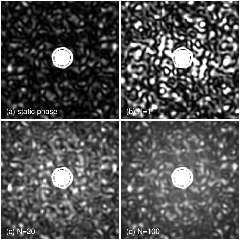
Figure 1: (a) A simulated (e.g.,   AO-corrected) PSF with a residual fitting error of 17 nm rms, producing a speckle pattern. (b) The PSF of a 20 nm rms independent phase error added to that used in (a). (c) the sum of 20 PSFs, each with the same residual error as (a) and independent 20 nm phase errors as in (b). (d) the sum of 100 PSFs as in (c) (See text for details).

Figure 2 shows this quantitatively. This is a plot of the image noise (measured as the standard deviation of the intensity values in an annulus) as a function of the number of seperate images added together. The noise initially declines rapidly as the speckles due to the white noise average together, but ultimately the noise reaches a plateau equal to the noise in an image having only the original fitting error common to all the images.

Figure 2: Image noise (measured as the standard deviation of the intensity values in an annulus) as a function of the number of seperate images added together. The noise eventually reaches a plateau equal to the noise in an image having only the original residual phase error. (See text for details).

On the face of it this appears to contradict the simulations of Stahl & Sandler (1995). However, the results are actually consistent with their work. Their initial simulations showed a long-lived speckle pattern that changed only on atmospheric timescales, which they attributed to a large wavefront error caused by time lags. (It may have been augmented by the lack of a wavefront reconstructor algorithm — instead, direct average phase measurements were applied directly to their simulated DM.) When they changed their AO model to incorporate a predictive controller with lower time lags, the speckle pattern began to change rapidly. The effect of the predictive controller, however, is not to decorrelate the speckles due to atmospheric timelag but to reduce the residual wavefront error due to this source and hence the total intensity of the long-lived speckle pattern; this left the short-lived speckles due to measurement error as the main remaining noise source. Stahl and Sandler did not demonstrate speckle decorrelation, but speckle suppression. One can always reduce speckle noise by reducing the corresponding wavefront error term; what one cannot do is change the timescale of a given speckle error term by introducing other zero-mean phase errors uncorrelated with the phase errors causing the original speckle. (In addition, the short timescales simulated by Stahl and Sandler may have masked longer-lived speckle effects, and the coarse sampling of their simulations may also have masked the real evolution of noise sources.)

5 Alternatives to speckle decorrelation

Each term in the series expansion of the PSF possesses distinct properties. Further work on characterizing the magnitude of the various terms (in both monochromatic and polychromatic cases), assuming either AO-corrected atmospheric turbulence or typical mirror aberrations is being done in order to assess how one might use the knowledge of these properties to improve dynamic range. The first order term has already been treated in the literature (Bloemhof et al., 2001; Boccaletti et al., 2002), although the second degree term $p_{2\ Strehl}$ is often the largest term close to the image core. Furthermore, when using speckle sweeping techniques, it is likely that ultimate dynamic range limits in the wings of the PSF are set by the other second degree term, $p_{2\ halo}$.

References

- Aime (2000) Aime, C. 2000, Journal of Optics A: Pure and Applied Optics, 2, 411
- Angel (1994) Angel, J. R. P. 1994, Nature, 368, 203
- Angel & Burrows (1995) Angel, R. & Burrows, A. 1995, Nature, 374, 678
- Bloemhof et al. (2001) Bloemhof, E. E., Dekany, R. G., Troy, M., & Oppenheimer, B. R. 2001, ApJ, 558, L71
- Boccaletti et al. (2000) Boccaletti, A., Moutou, C., & Abe, L. 2000, A&AS, 141, 157
- Boccaletti et al. (2002) Boccaletti, A., Riaud, P., & Rouan, D. 2002, PASP, 114, 132
- Canales & Cagigal (2000) Canales, V. F. & Cagigal, M. P. 2000, A&AS, 145, 445
- Labeyrie (1995) Labeyrie, A. 1995, A&A, 298, 544
- Nakajima (1994) Nakajima, T. 1994, ApJ, 425, 348
- Racine et al. (1999) Racine, R. ., Walker, G. A. H., Nadeau, D., Doyon, R. ., & Marois, C. 1999, PASP, 111, 587
- Saha (2002) Saha, S. K. 2002, Reviews of Modern Physics, 74, 551, astro-ph/0202115
- Sivaramakrishnan et al. (2001) Sivaramakrishnan, A., Koresko, C. D., Makidon, R. B., Berkefeld, T., & Kuchner, M. J. 2001, ApJ, 552, 397
- Stahl & Sandler (1995) Stahl, S. M. & Sandler, D. G. 1995, ApJ, 454, L153
- Woolf & Angel (1998) Woolf, N. & Angel, J. R. 1998, ARA&A, 36, 507