HARM: A Numerical Scheme for General Relativistic Magnetohydrodynamics

Abstract

We describe a conservative, shock-capturing scheme for evolving the equations of general relativistic magnetohydrodynamics. The fluxes are calculated using the Harten, Lax, and van Leer scheme. A variant of constrained transport, proposed earlier by Tóth, is used to maintain a divergence free magnetic field. Only the covariant form of the metric in a coordinate basis is required to specify the geometry. We describe code performance on a full suite of test problems in both special and general relativity. On smooth flows we show that it converges at second order. We conclude by showing some results from the evolution of a magnetized torus near a rotating black hole.

1 Introduction

Quasars, active galactic nuclei (AGN), X-ray binaries, gamma-ray bursts, and core-collapse supernovae are all likely powered by a central engine subject to strong gravity, strong electromagnetic fields, and rotation. For convenience, we will refer to this class of objects as relativistic magneto-rotators (RMRs). RMRs are among the most luminous objects in the universe and are therefore the center of considerable theoretical attention. Unfortunately the governing physical laws for RMRs, while well known, are nonlinear, time-dependent, and intrinsically multidimensional. This has stymied development of a first-principles theory for their evolution and observational appearance and strongly motivates a numerical approach.

To fully understand RMR structure, one must be able to follow the interaction of a non-Maxwellian plasma with a relativistic gravitational field, a strong electromagnetic field, and possibly a strong radiation field as well. This general problem remains beyond the reach of today’s algorithms and computers. A useful first step, however, might be to study these objects in a nonradiating magnetohydrodynamic (MHD) model. In this case the plasma can be treated as a fluid, greatly reducing the number of degrees of freedom, and the radiation field can be ignored. The relevance of this approximation must be evaluated in astrophysical context and will not be considered here.

We were motivated, therefore, to develop a method for integrating the equations of ideal, general relativistic MHD (GRMHD), and that method is described in this paper. This is in a sense well-trodden ground: many schemes have already been developed for relativistic fluid dynamics. What has not existed until recently is a scheme that: (1) includes magnetic fields; (2) has been fully verified and convergence tested; (3) is stable and capable of integrating a flow over many dynamical times. A pioneering GRMHD code has been developed by Koide and collaborators (e.g. Koide et al. (2002), Koide, Shibata, & Kudoh (1999), Koide et al. (2000), Meier, Koide, & Uchida (2001)). Our code code differs in that we have subjected it to a fuller series of tests (described in this paper), we can perform longer integrations than the rather brief simulations described in the published work of Koide’s group, and our code explicitly maintains the divergence-free constraint on the magnetic field. A GRMHD Godunov scheme based on a Roe-type approximate Riemann solver has been developed by Komissarov and described in a conference proceeding (Komissarov, 2001).

A rather complete review of numerical approaches to relativistic fluid dynamics is given by Martí & Muller (1999) and Font (2000). The first numerical GRMHD scheme that we are aware of is by Wilson (1977), who integrated the GRMHD equations in axisymmetry near a Kerr black hole. While it was recognized throughout the 1970s that relativistic MHD would be relevant to problems related to black hole accretion (particularly following the seminal work of Blandford & Znajek (1977) and Phinney (1983); see also Punsly (2001)), no further work appeared until Yokosawa (1993). The discovery by Balbus & Hawley (1991) that magnetic fields play a crucial role in regulating accretion disk evolution (reviewed in Balbus & Hawley (1998)) and the absence of purely hydrodynamic means for driving accretion in disks (Balbus & Hawley, 1998) further motivated the development of relativistic MHD schemes. More recently there have been several efforts to develop GRMHD codes, including the already-mentioned work by Koide and collaborators and by Komissarov. A ZEUS-like scheme for GRMHD has also been developed and is described in a companion paper (de Villiers & Hawley, 2002).

Special relativistic MHD (SRMHD) is the foundation for any GRMHD scheme, although there are nontrivial problems in making the transition to full general relativity. SRMHD schemes have been developed by Van Putten (1993); Balsara (2001); Koldoba et al. (2002); Komissarov (1999) and Del Zanna et al. (2002). We were particularly influenced by the clear development of the fundamental equations in Komissarov (1999) for his Godunov SRMHD scheme based on a Roe-type approximate Riemann solver, and by the work of Del Zanna & Bucciantini (2002) and Del Zanna et al. (2002) who chose to use the simple approximate Riemann solver of Harten et al. (1983) in their special relativistic hydrodynamics and SRMHD schemes, respectively.

Our numerical scheme is called HARM, for High Accuracy Relativistic Magnetohydrodynamics. In the next section we develop the basic equations in the form used for numerical integration in HARM (§2). In §3 we describe the basic algorithm. In §4 we describe the performance of the code on a series of test problems. In §5 we describe a sample evolution of a magnetized torus near a rotating black hole.

2 A GRMHD Primer

The equations of general relativistic MHD are well known, but for clarity we will develop them here in the same form used in numerical integration. Unless otherwise noted $c=1$ and we follow the notational conventions of Misner, Thorne, & Wheeler (1973), hereafter MTW. The reader may also find it useful to consult Anile (1989).

The first governing equation describes the conservation of particle number:

$$(nu^{\mu})_{;\mu}=0.$$ (1)

Here $n$ is the particle number density and $u^{\mu}$ is the four-velocity. For numerical purposes we rewrite this in a coordinate basis, replacing $n$ with the “rest-mass density” $\rho=mn$, where $m$ is the mean rest-mass per particle:

$${1\over{{\sqrt{-g}}}}\partial_{\mu}({\sqrt{-g}}\,\rho u^{\mu})=0.$$ (2)

Here $g\equiv Det(g_{\mu\nu})$.

The next four equations express conservation of energy-momentum:

$${T^{\mu}}_{\nu;\mu}=0,$$ (3)

where ${T^{\mu}}_{\nu}$ is the stress-energy tensor. In a coordinate basis,

$$\partial_{t}\left({\sqrt{-g}}\,{T^{t}}_{\nu}\right)=-\partial_{i}\left({\sqrt{-g}}\,{T^{i}}_{\nu}\right)+{\sqrt{-g}}\,{T^{\kappa}}_{\lambda}\,{\Gamma^{\lambda}}_{\nu\kappa},$$ (4)

where $i$ denotes a spatial index and ${\Gamma^{\lambda}}_{\nu\kappa}$ is the connection.

The energy-momentum equations have been written with the free index down for a reason. Symmetries of the metric give rise to conserved currents. In the Kerr metric, for example, the axisymmetry and stationary nature of the metric give rise to conserved angular momentum and energy currents. In general, for metrics with an ignorable coordinate $x^{\mu}$ the source term on the right hand side of the evolution equation for $T^{t}_{\mu}$ vanish. These source terms do not vanish when the equation is written with both indices up.

The stress-energy tensor for a system containing only a perfect fluid and an electromagnetic field is the sum of a fluid part,

$$T^{\mu\nu}_{\rm fluid}=(\rho+u+p)u^{\mu}u^{\nu}+pg^{\mu\nu},$$ (5)

(here $u\equiv$ internal energy and $p\equiv$ pressure) and an electromagnetic part,

$$T^{\mu\nu}_{\rm EM}=F^{\mu\alpha}F^{\nu}_{\alpha}-{1\over{4}}g^{\mu\nu}F_{\alpha\beta}F^{\alpha\beta}.$$ (6)

Here $F^{\mu\nu}$ is the electromagnetic field tensor (MTW: “Faraday”), and for convenience we have absorbed a factor of $\sqrt{4\pi}$ into the definition of $F$.

The electromagnetic portion of the stress-energy tensor simplifies if we adopt the ideal MHD approximation, in which the electric field vanishes in the fluid rest frame due to the high conductivity of the plasma (“${\bf E}+{\bf v}\times{{\bf B}}=0$”). Equivalently the Lorentz force on a charged particle vanishes in the fluid frame:

$$u_{\mu}F^{\mu\nu}=0.$$ (7)

It is convenient to define the magnetic field four-vector

$$b^{\mu}\equiv{1\over{2}}\epsilon^{\mu\nu\kappa\lambda}u_{\nu}F_{\lambda\kappa},$$ (8)

where $\epsilon$ is the Levi-Civita tensor. Recall that (following the notation of MTW) $\epsilon^{\mu\nu\lambda\delta}=-{1\over{{\sqrt{-g}}}}[\mu\nu\lambda\delta]$, where $[\mu\nu\lambda\delta]$ is the completely antisymmetric symbol and $=0,1,$ or $-1$. These can be combined (with the aid of identity 3.50h of MTW):

$$F^{\mu\nu}=\epsilon^{\mu\nu\kappa\lambda}u_{\kappa}b_{\lambda}.$$ (9)

Substitution and some manipulation (using identities 3.50 of MTW and $b_{\mu}u^{\mu}=0$; the latter follows from the definition of $b_{\mu}$ and the antisymmetry of $F$) yields

$$T^{\mu\nu}_{\rm EM}=b^{2}u^{\mu}u^{\nu}+{1\over{2}}b^{2}g^{\mu\nu}-b^{\mu}b^{\nu}.$$ (10)

Notice that the last two terms are nearly identical to the nonrelativistic MHD stress tensor, while the first term is higher order in $v/c$. To sum up,

$$T^{\mu\nu}_{\rm MHD}=(\rho+u+p+b^{2})u^{\mu}u^{\nu}+(p+{1\over{2}}b^{2})g^{\mu\nu}-b^{\mu}b^{\nu}$$ (11)

is the MHD stress-energy tensor.

The electromagnetic field evolution is given by the source-free part of Maxwell’s equations

$$F_{\mu\nu,\lambda}+F_{\lambda\mu,\nu}+F_{\nu\lambda,\mu}=0.$$ (12)

The rest of Maxwell’s equations determine the current

$$J^{\mu}={F^{\mu\nu}}_{;\nu},$$ (13)

and are not needed for the evolution, as in nonrelativistic MHD.

Maxwell’s equations can be written in conservative form by taking the dual of eq.(12):

$${F^{*\mu\nu}}_{;\nu}=0.$$ (14)

Here $F^{*}_{\mu\nu}={1\over{2}}\epsilon_{\mu\nu\kappa\lambda}F^{\kappa\lambda}$ is the dual of the electromagnetic field tensor (MTW: “Maxwell”). In ideal MHD

$$F^{*\mu\nu}=b^{\mu}u^{\nu}-b^{\nu}u^{\mu},$$ (15)

which can be proved by taking the dual of eq.(9).

The components of $b^{\mu}$ are not independent, since $b^{\mu}u_{\mu}=0$. Following, e.g., Komissarov (1999), it is useful to define the magnetic field three-vector $B^{i}=F^{*it}$. In terms of $B^{i}$,

$$b^{t}=B^{i}u^{\mu}g_{i\mu},$$ (16)

$$b^{i}=(B^{i}+b^{t}u^{i})/u^{t}.$$ (17)

The space components of the induction equation then reduce to

$${\partial}_{t}({\sqrt{-g}}B^{i})=-{\partial}_{j}({\sqrt{-g}}\,(b^{j}u^{i}-b^{i}u^{j}))$$ (18)

and the time component reduces to

$${1\over{{\sqrt{-g}}}}{\partial}_{i}({\sqrt{-g}}\,B^{i})=0,$$ (19)

which is the no-monopoles constraint. The appearance of $B^{i}$ in these last two equations are what motivates the introduction of the field three-vector in the first place.

To sum up, the fundamental equations as used in HARM are: the particle number conservation equation (2); the four energy-momentum equations (4), written in a coordinate basis and using the MHD stress-energy tensor of equation (11); and the induction equation (18), subject to the constraint (19). These hyperbolic equations are written in conservation form, and so can be solved numerically by well-known techniques.

3 Numerical Scheme

There are many possible ways to numerically integrate the GRMHD equations. A first, zeroth-order choice is between conservative and nonconservative schemes. Nonconservative schemes such as ZEUS (Stone & Norman, 1992) have enjoyed wide use in numerical astrophysics. They permit the integration of an internal energy equation rather than a total energy equation. This can be advantageous in regions of a flow where the internal energy is small compared to the total energy (highly supersonic flows), which is a common situation in astrophysics. A nonconservative scheme for GRMHD following a ZEUS-like approach has been developed and is described in a companion paper (de Villiers & Hawley, 2002).

We have decided to write a conservative scheme. One advantage of this choice is that in one dimension, total variation stable schemes are guaranteed to converge to a weak solution of the equations by the Lax-Wendroff theorem (Lax & Wendroff, 1960) and by a theorem due to LeVeque (1998). While no such guarantee is available for multidimensional flows, this is a reassuring starting point. Furthermore, one is guaranteed that a conservative scheme in any number of dimensions will satisfy the jump conditions at discontinuities. This is not true in artificial viscosity based nonconservative schemes, which are also known to have trouble in relativistic shocks (Norman & Winkler, 1986). Conservative schemes for GRMHD have also been developed by Komissarov (2001) and by Koide, Shibata, & Kudoh (1999).

A conservative scheme updates a set of “conserved” variables at each timestep. Our vector of conserved variables is

$${\bf U}\equiv{\sqrt{-g}}(\rho u^{t},T^{t}_{t},T^{t}_{i},B^{i}).$$ (20)

These are updated using fluxes ${\bf F}$. We must also choose a set of “primitive” variables, which are interpolated to model the flow within zones. We use variables with a simple physical interpretation:

$${\bf P}=(\rho,u,v^{i},B^{i}).$$ (21)

Here $v^{i}=u^{i}/u^{t}$ is the 3-velocity. The functions ${\bf U}({\bf P})$ and ${\bf F}({\bf P})$ are analytic, but the inverse operations (so far as we can determine) are not. There is also no simple expression for ${\bf F}({\bf U})$.

To evaluate ${\bf U}({\bf P})$ and ${\bf F}({\bf P})$ one must find $u^{t}$ and $b^{\mu}$ from $v^{i}$ and $B^{i}$. To find $u^{t}$, solve the quadratic equation $g_{\mu\nu}u^{\mu}u^{\nu}=-1$. Next use equations (16) and (17) to find $b^{\mu}$; these require only multiplications and additions. The remainder of the calculation of ${\bf U}({\bf P})$ and ${\bf F}({\bf P})$ requires raising and lowering of indices followed by direct substitution in equation (11) to find the components of the MHD stress-energy tensor.

Since we update ${\bf U}$ rather than ${\bf P}$, we must solve for ${\bf P}({\bf U})$ at the end of each timestep. We use a multidimensional Newton-Raphson routine with the value of ${\bf P}$ from the last timestep as an initial guess. Since $B^{i}$ can be obtained analytically, only 5 equations need to be solved. The Newton-Raphson method requires an expensive evaluation of the Jacobian $\partial{\bf U}/\partial{\bf P}$. In practice we evaluate the Jacobian analytically. It is possible to evaluate the Jacobian by numerical derivatives, but this is both expensive and a source of numerical noise.

The evaluation of ${\bf P}({\bf U})$ is at the heart of our numerical scheme; the procedure must be robust. We have found that it is crucial that the errors (differences between the current and target values of ${\bf U}$) used to evaluate convergence in the Newton-Raphson scheme be properly normalized. We normalized the errors with ${\sqrt{-g}}\rho u^{t}$.

To evaluate ${\bf F}$ we use a MUSCL type scheme with “HLL” fluxes (Harten et al., 1983). The fluxes are defined at zone faces. A slope-limited linear extrapolation from the zone center gives ${\bf P}_{R}$ and ${\bf P}_{L}$, the primitive variables at the right and left side of each zone interface. We have implemented the monotonized central (“Woodward”, or “MC”) limiter, the van Leer limiter, and the minmod limiter; unless otherwise stated, the tests described here use the MC limiter, which is the least diffusive of the three.

From ${\bf P}_{R},{\bf P}_{L}$, calculate the maximum left and rightgoing wave speeds $c_{\pm,R},c_{\pm,L}$, and the fluxes ${\bf F}_{R}={\bf F}({\bf P}_{R})$ and ${\bf F}_{L}={\bf F}({\bf P}_{L})$. Defining $c_{max}\equiv{\rm MAX}(0,c_{+,R},c_{+,L})$ and $c_{min}\equiv-{\rm MIN}(0,c_{-,R},c_{-,L})$, the HLL flux is then

$${\bf F}={c_{min}{\bf F}_{R}+c_{max}{\bf F}_{L}-c_{max}c_{min}({\bf U}_{R}-{\bf U}_{L})\over{c_{max}+c_{min}}}$$ (22)

If $c_{max}=c_{min}$, the HLL flux becomes the so-called local Lax-Friedrichs flux.

3.1 Constrained Transport

The pure HLL scheme will not preserve any numerical representation of ${\bf\nabla}\cdot{\bf B}=0$. An incomplete list of options for handling this constraint numerically includes: (1) ignore the production of monopoles by truncation error and hope for the best (in our experience this causes the scheme to fail in any complex flow); (2) introduce a divergence-cleaning step (this entails solving an elliptic equation at each timestep); (3) use an Evans & Hawley (1988) type constrained transport scheme (this requires a staggered mesh, so that the magnetic field components are zone face centered); (4) introduce a diffusion term that causes numerically generated monopoles to diffuse away (Marder (1987); this typically leaves a monopole field with rms value somewhat larger than the truncation error).

We have chosen a fifth option, a version of constrained transport that can be used with a zone-centered scheme. This idea was introduced by one of us in Tóth (2000), where it is called the flux-interpolated constrained transport (or “flux-CT”) scheme . It preserves a numerical representation of ${\bf\nabla}\cdot{\bf B}=0$ by smoothing the fluxes with a special operator. The disadvantage of this method is that it is more diffusive than the “bare”, unconstrained scheme. The advantage is that it is extremely simple.

To clarify how zone-centered constrained transport works we now give a specific example for a special relativistic problem in Cartesian coordinates $t,x,y$. To fix notation, write the induction equation as

$${\partial}_{t}B^{i}=-{\partial}_{j}F^{j}_{i},$$ (23)

where we have used ${\sqrt{-g}}=1$ and the fluxes $F^{j}_{i}$ are

$$\begin{array}[]{rcl}F^{x}_{x}&=&0\\ F^{y}_{y}&=&0\\ F^{y}_{x}&=&b^{y}u^{x}-b^{x}u^{y}\\ F^{x}_{y}&=&b^{x}u^{y}-b^{y}u^{x}=-F^{y}_{x}\end{array}$$ (24)

Notice that the fluxes are centered at different locations on the grid: $F^{x}$ fluxes live on the $x$ face of each zone at grid location $i-1/2,j$ (we use $i,j$ to denote the center of each zone), while $F^{y}$ fluxes live on the $y$ face at $i,j-1/2$. The smoothing operator replaces the numerical (HLL-derived) $F_{i}^{j}$ with $\tilde{F}^{j}_{i}$, defined by

$$\begin{array}[]{rcl}\tilde{F}^{x}_{x}(i-1/2,j)&=&0\\ \tilde{F}^{y}_{y}(i,j-1/2)&=&0\\ \tilde{F}^{y}_{x}(i,j-1/2)&=&{1\over{8}}\Bigl{[}2F^{y}_{x}(i,j-1/2)\\ &&+F^{y}_{x}(i+1,j-1/2)+F^{y}_{x}(i-1,j-1/2)\\ &&-F^{x}_{y}(i-1/2,j)-F^{x}_{y}(i+1/2,j)\\ &&-F^{x}_{y}(i-1/2,j-1)-F^{x}_{y}(i+1/2,j-1)\Bigr{]}\\ \tilde{F}^{x}_{y}(i-1/2,j)&=&{1\over{8}}\Bigl{[}2F^{x}_{y}(i-1/2,j)\\ &&+F^{x}_{y}(i-1/2,j+1)+F^{x}_{y}(i-1/2,j-1)\\ &&-F^{y}_{x}(i,j-1/2)-F^{y}_{x}(i,j+1/2)\\ &&-F^{y}_{x}(i-1,j-1/2)-F^{y}_{x}(i-1,j+1/2)\Bigr{]}\end{array}$$ (25)

It is a straightforward but tedious exercise to verify that this preserves the following corner-centered numerical representation of ${\bf\nabla}\cdot{\bf B}$:

$$\begin{array}[]{rcl}{\bf\nabla}\cdot{\bf B}&=&\left(B^{x}(i,j)+B^{x}(i,j-1)-B^{x}(i-1,j)-B^{x}(i-1,j-1)\right)/(2\Delta x)\\ &&+\left(B^{y}(i,j)+B^{y}(i-1,j)-B^{y}(i,j-1)-B^{y}(i-1,j-1)\right)/(2\Delta y),\end{array}$$ (26)

where $\Delta x$ and $\Delta y$ are the grid spacing.

3.2 Wave Speeds

The HLL approximate Riemann solver does not require eigenvectors of the characteristic matrix (as would a Roe-type scheme), but it does require the maximum and minimum wave speed (eigenvalues). These wave speeds are also required to fix the timestep via the Courant conditions. The relevant speed is the phase speed “$\omega/k$” of the wave, and it turns out that only speeds for waves with wavevectors aligned along coordinate axes are required. Suppose, for example, that one needs to know how rapidly signals propagate in the fluid along the $x_{1}$ direction. First, find a wavevector $k_{\mu}=(-\omega,k_{1},0,0)$, that satisfies the dispersion relation for the mode in question: $D(k_{\mu})=0$. Then the wave speed is simply $\omega/k_{1}$.

The dispersion relation $D(k_{\mu})=0$ for MHD waves has a simple form in a comoving frame. In terms of the relativistic sound speed $c_{s}^{2}=({\partial}(\rho+u)/{\partial}p)_{s}^{-1}=\gamma p/w$, (the last holds only if $p=(\gamma-1)u$) and the relativistic Alfvén velocity ${\bf v}_{\rm A}={\bf B}/\sqrt{{\mathcal{E}}}$, where ${\mathcal{E}}=b^{2}+w$ and $w\equiv\rho+u+p$, the dispersion relation is

$$\begin{array}[]{l}\omega\left(\omega^{2}-({\bf k}\cdot{\bf v}_{\rm A})^{2}\right)\times\\ \left(\omega^{4}+\omega^{2}\,\left(k^{2}({\bf v}_{\rm A}^{2}+c_{s}^{2}(1-{\bf v}_{\rm A}^{2}/c^{2}))+c_{s}^{2}({\bf k}\cdot{\bf v}_{\rm A})^{2}/c^{2}\right)+k^{2}c_{s}^{2}({\bf k}\cdot{\bf v}_{\rm A})^{2}\right)=0,\end{array}$$ (27)

Here $c$ is the (temporarily reintroduced) speed of light. The first term is the zero frequency entropy mode, the second is the Alfvén mode, and the third contains the fast and slow modes. The eighth mode is eliminated by the no-monopoles constraint.

The relativistic sound speed asymptotes to $c\sqrt{\gamma-1}=c/\sqrt{3}$ for $\gamma=4/3$, and the Alfvén speed asymptotes to $c$. In the limit that $B^{2}/\rho\gg 1$ and $p/\rho\sim\ll 1$, the GRMHD equations are a superset of the time-dependent, force-free electrodynamics equations recently discussed by Komissarov (2002b); these contain fast modes and Alfvén modes that move with the speed of light. They are indistinguishable from vacuum electromagnetic modes only when their wavevector is oriented along the magnetic field.

To find the maximum wave speeds we need to evaluate the comoving-frame dispersion relation for the fast wave branch from coordinate frame quantities. This is straightforward because the dispersion relation depends on scalars, which can be evaluated in any frame: $\omega=k_{\mu}u^{\mu}$; $k^{2}=K_{\mu}K^{\mu}$, where $K_{\mu}=(g_{\mu\nu}+u_{\mu}u_{\nu})k^{\nu}$ is the part of the wavevector normal to the fluid 4-velocity; ${\bf v}_{\rm A}^{2}=b_{\mu}b^{\mu}/{\mathcal{E}}$; $({\bf k}\cdot{\bf v}_{\rm A})=k_{\mu}b^{\mu}/\sqrt{{\mathcal{E}}}$. The relevant portion of the dispersion relation (for fast and slow modes) is thus a fourth order polynomial in the components of $k_{\mu}$. This can be solved either analytically or by standard numerical methods. The two fast mode speeds are then used as $c_{max}$ and $c_{min}$ in the HLL fluxes.

We have found it convenient to replace the full dispersion relation by an approximation:

$$\omega^{2}=({\bf v}_{\rm A}^{2}+c_{s}^{2}(1-{\bf v}_{\rm A}^{2}/c^{2}))k^{2}.$$ (28)

This overestimates the maximum wavespeed by a factor $\leq 2$ in the comoving frame. The maximum error occurs for ${\bf k}\parallel{\bf v}_{\rm A},v_{A}/c_{s}=1,$ and $v_{A}\ll c$, and it is usually much less, particularly if the fluid is moving super-Alfvénically with respect to the grid. This approximation is convenient because it is quadratic in $k_{\mu}$, and so can be solved more easily.

3.3 Implementation Notes

For completeness we now give some details of the implementation of the algorithm.

Time Stepping. Our scheme is made second order in time by taking a half-step from $t^{n}$ to $t^{n+1/2}$, evaluating ${\bf F}({\bf P}(t^{n+1/2}))$, and using that to update ${\bf U}(t^{n})$ to ${\bf U}(t^{n+1})$.

Modification of Energy Equation. A direct implementation of the energy equation can be inaccurate because the magnetic and internal energy density can be orders of magnitude smaller than the rest mass density. To avoid this we subtract the particle number conservation equation from the energy equation, i.e., we evolve

$${\partial}_{t}({\sqrt{-g}}(T^{t}_{t}+\rho u^{t}))=-{\partial}_{i}({\sqrt{-g}}(T^{i}_{t}+\rho u^{i}))+{\sqrt{-g}}T^{\kappa}_{\lambda}\Gamma^{\lambda}_{t\kappa}.$$ (29)

In the nonrelativistic limit, this procedure subtracts the rest mass energy density from the total energy density.

Specification of Geometric Quantities. In two dimensions we need to evaluate $g_{\mu\nu},g^{\mu\nu},$ and ${\sqrt{-g}}$ at four points in every grid zone (the center, two faces, and one corner) and $\Gamma^{\mu}_{\nu\lambda}$ at the zone center. It would be difficult to accurately encode analytic expressions for all these quantities. HARM is coded so that an analytic expression need only be provided for $g_{\mu\nu}$; all other geometric quantities are calculated numerically. The connection, for example, is obtained to sufficient accuracy by numerical differentiation of the metric. This minimizes the risk of coding errors in specifying the geometry. It also minimizes coordinate dependent code, making it relatively easy to change coordinate systems. Minimal coordinate dependence, besides following the spirit of general relativity, enables one to perform a sort of fixed mesh refinement by adapting the coordinates to the problem at hand. For example, near a Kerr black hole we use $\log(r)$ as the radial coordinate instead of the usual Boyer-Lindquist $r$, and this concentrates numerical resolution toward the horizon, where it is needed.

Density and Internal Energy Floors. Negative densities and internal energies are forbidden by the GRMHD equations, but numerically nothing prevents their appearance. In fact, negative internal energies are common in numerical integrations with large density or pressure contrast. Following common practice, we prevent this by introducing “floor” values for the density and internal energy. These floors are enforced after the half-step and the full step. They preserve velocity but do not conserve rest mass or energy-momentum.

Outflow Boundary Conditions. In the rotating black hole calculations described below we use outflow boundary conditions at the inner and outer radial boundaries. The usual implementation of outflow boundary conditions is to simply copy the primitive variables from the boundary zones into the ghost zones. This can result in unphysical values of the primitive variables in the ghost zones– for example, velocities that lie outside the light cone– because of variations in the metric between the boundary and ghost zones.

We have experimented with a variety of schemes for projecting variables into the ghost zones in the context of black hole accretion flow calculations (described in §5). We find that some are more robust than others. The most robust extrapolates the density, internal energy, and radial magnetic field according to

$$P({\rm ghost})=P({\rm boundary}){\sqrt{-g}}({\rm boundary})/{\sqrt{-g}}({\rm ghost}),$$ (30)

the $\theta$ and $\phi$ components of the velocity and magnetic field according to

$$P({\rm ghost})=P({\rm boundary})(1.-\Delta r/r),$$ (31)

and the radial velocity according to

$$P({\rm ghost})=P({\rm boundary})(1.+\Delta r/r).$$ (32)

The extrapolation of $\theta$ and $\phi$ components of magnetic field and velocity results in weak damping of these components near the boundary. Slightly different choices of the extrapolation coefficients (i.e. $(1.-2\Delta r/r)$) are much less robust.

Performance. We have implemented both serial and parallel versions of the code. In serial mode the code integrates the black hole accretion problem (described in §5) at $\approx 54,000$ zone cycles per second on a 2.4 GHz Intel Pentium 4, when compiled using the Intel C compiler. The parallel code was implemented using MPI.

4 Code Verification

Here we present a test suite for verifying a GRMHD code. The tests are nonrelativistic, special and general relativistic, and one and two dimensional. The list of problems for which there are known, exact solution is short, since exact solutions of multidimensional GRMHD problems are algebraically complicated. This list of test problems was developed in collaboration with J. Hawley and J.-P. de Villiers. Unless otherwise stated we set $\gamma=4/3$ and $c=1$.

4.1 Linear Modes

This first test considers the evolution of a small amplitude wave in two dimensions. The unperturbed state is $\rho=1$, $p=1$, $u^{i}=0$, $B^{y}=B^{z}=0$, $B^{x}=B^{x}_{0}$. The basic state is parametrized by $\alpha=(B^{x}_{0})^{2}/(\rho c^{2})$; our fiducial test runs have $\alpha=1$. Onto this basic state we introduce a perturbation of the form $\exp(i{\bf k}\cdot{\bf x}-i\omega({\bf k})t)$, where $(k_{x},k_{y})=(2\pi,2\pi)$, and the amplitude is fixed by $\delta B^{y}=10^{-4}B^{x}_{0}$. The computational domain is $x,y\in[0,1),[0,1)$, and the boundary conditions are periodic. The wave is either slow, Alfvénic, or fast.

This test exercises almost all terms in the governing equations. The numerical resolution is $(N_{x},N_{y})\equiv N(5,4)$ zones, and the integration runs for a single wave period $2\pi/\omega$, so that a perfect scheme would return the simulation to its original state. We measure the ${\mathcal{L}}_{1}$ norm of the difference between the final state and the initial state for each primitive variable. For example, we measure

$${\mathcal{L}}_{1}(\delta\rho)=\int dxdy|\rho({\rm t=0})-\rho({\rm t=2\pi/\omega})|.$$ (33)

for the density.

All primitive variables exhibit similar convergence properties (as they must, since with the exception of the magnetic field, they are tightly coupled together). In Figures 1, 2, and 3 we present the ${\mathcal{L}}_{1}$ norm of the error for runs using the monotonized central limiter and a Courant number of $0.8$, in addition to the results for the minmod limiter. These runs have $\alpha=1$. Figure 1 shows the results for the slow wave, Figure 2 for the Alfvén wave, and Figure 3 for the fast wave. Evidently the convergence rate asymptotes to second order, although more slowly for the minmod limiter.

The code performs similarly well over a range of $\alpha$, provided only that $\delta B^{2}/2\ll p$, which is necessary for the wave to be in the linear regime. We have been unable to find a value of $B^{x}_{0}$ where the code fails completely for a linear amplitude disturbance, although for very large values of $B^{x}_{0}$ the evolution becomes inaccurate because of numerical noise in the evaluation of ${\bf P}({\bf U})$.

4.2 Nonlinear Waves

Komissarov (1999) has proposed a suite of one-dimensional nonlinear tests for special relativistic MHD. Komissarov presents a total of 9 tests (see his Table 1). The nonlinear Alfvén wave (test 5), and the compound wave (test 6) cannot be reconstructed without a separate derivation of the exact analytic solution, and we will not provide that here. For the remaining tests Komissarov’s Table 1 contains several misprints that are corrected in Komissarov (2002a). Our code is able to integrate each of Komissarov’s remaining 7 tests, although in some cases we must reduce the Courant number (usually $0.8$) or resort to the slightly more robust van Leer slope limiter. Tests that required special treatment are: fast shock (Courant number $=0.5$); shock tube 1 (Courant number $=0.3$, van Leer limiter); shock tube 2 (Courant number $=0.5$); collision (Courant number $=0.3$; van Leer limiter).

Figures 4 and 5 show the run of $\rho$ and $u^{x}$, respectively, for all 7 tests. These may be compared with Komissarov’s figures. Notice that, unlike Komissarov, we have in all cases set $N_{x}=400$ and $x\in(-2,2)$. We have not obtained the exact solutions used by Komissarov, but the solutions can still be checked quantitatively. For example, the slow shock wave speed is $0.5$; since the calculation ends at $t=2$ the slow shock front should be, and is, located at $x\approx 1.0$. The fast shock speed is $0.2$, so at $t=2.5$ the fast shock wave front should be, and is, located at $x\approx 0.5$.

There are artifacts evident in the figures. In particular there is ringing near the base of the switch-on and switch-off rarefaction waves. This is common and is seen in Komissarov’s results as well. In addition the narrow, Lorentz-contracted shell of material behind the shock in shock tube 1 is poorly resolved; the correct shell density is $\approx 0.88$ but a resolution of $N_{x}>800$ is required to find this result to an accuracy of a few percent. There is also a transient associated with the fast shock that propagates off the grid and so is not visible in Figures 4 and 5.

A complete set of nonlinear wave tests for one dimensional nonrelativistic MHD was developed by Ryu & Jones (1995) (hereafter RJ). We can run these under HARM by rescaling the speed of light to $c=10^{2}$ in code units, where all velocities in the tests are ${\mathcal{O}}(1)$. This should lead to results that agree with RJ to ${\mathcal{O}}(v/c)\approx 1\%$. The results can be checked quantitatively by comparison to the tables provided by RJ.

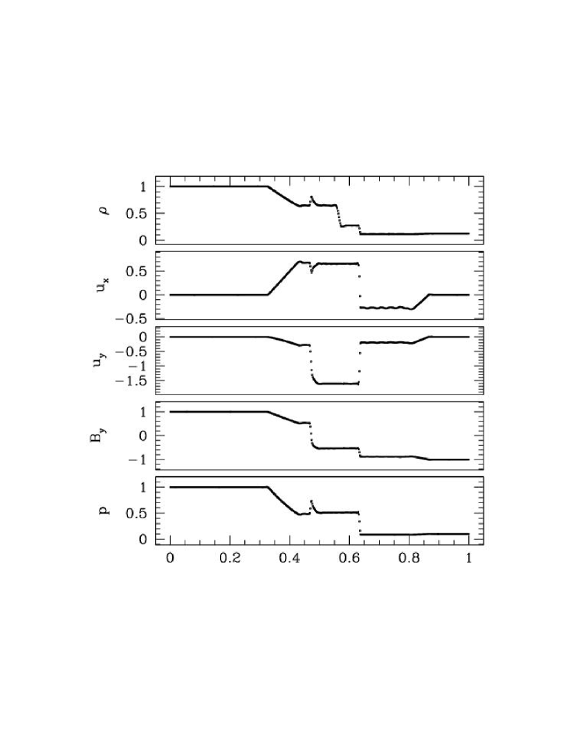
Figure 6: Snapshot of the final state in HARM’s integration of Ryu & Jones test 5A (a version of the Brio & Wu shock tube) but with $c=100$. The figure shows primitive variable values at $t=0.15$. Quantitative agreement is found to within $\approx 1\%$, as expected.

Figure 6 shows our results for RJ test 5A, which is a version of the familiar Brio & Wu (1988) magnetized shock tube test. Like RJ we use $512$ zones between $x=0$ and $x=1$, and we measure the results at $t=0.15$. To compare to RJ quantitatively, consider $u_{x}$ in the region behind the fast rarefaction wave, near $x=0.7$. RJ report $u_{x}=-0.277$ here, while we measure $u_{x}=-0.273$, which differs by $1\%$, as expected. Similar agreement is found for the other variables. The most unsatisfactory feature of the solution is the visible post-shock oscillations. The amplitude of these features varies, depending on the Courant number (here $0.9$) and the choice of slope limiter (here MC).

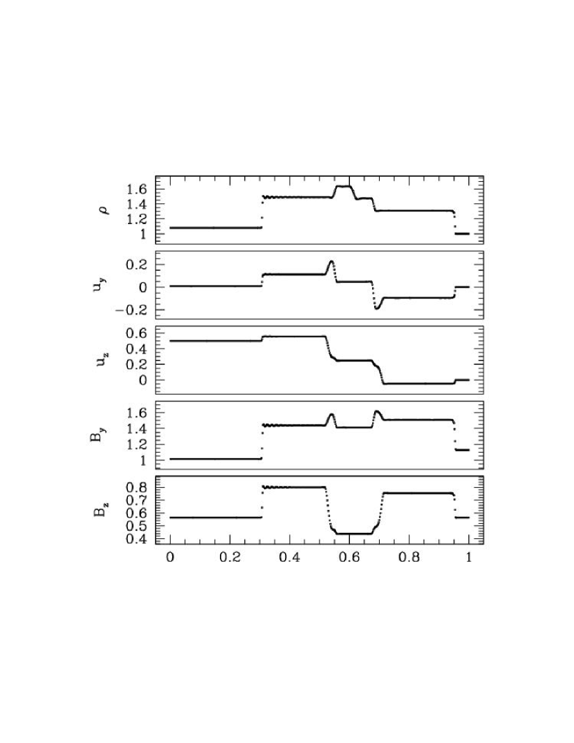
Figure 7: Snapshot of the final state in HARM’s integration of Ryu & Jones test 2A, with $c=100$.

Figure 7 shows our results for RJ test 2A. In the region near $x=0.6$, RJ report that $B_{y}=1.4126$, and we find essentially exact agreement ($B_{y}=1.41262$) after averaging over a small region near $x=0.6$. This test has two pairs of closely spaced slow shocks and rotational discontinuities that are difficult to resolve, and our scheme barely obtains the correct peak values of $u_{y}$ and $B_{y}$, even though there are about $20$ zones inside the “horns” visible in the $B_{y}$ panel of the figure.

4.3 Transport

This special relativistic test evolves a disk of enhanced density moving at an angle to the grid until it returns to its original position. The computation is carried out in a domain $x,y\in[-0.5,0.5),[-0.5,0.5)$ and the boundary conditions are periodic. The initial state has $v^{x}=v^{y}=0.7$, or $u^{x}=u^{y}\approx 4.95$, corresponding to $u^{t}\approx 7.07$. The initial density $\rho=1$ except in a disk at $r<r_{s}=0.45$, where $\rho=3/2+\cos(2\pi r/r_{s})$. The initial pressure $p=1$, and the initial magnetic field is zero. The test is run until $t=10/7$, when the system should return exactly to its initial state.

Numerically, we use the monotonized central limiter and set the Courant number to $0.8$. The resolution is fixed so that $N_{x}=5N_{y}/4$. Figure 8 shows the $L_{1}$ norm of the error in $\rho$ as a function of $x$ resolution. The convergence rate asymptotes to second order.

4.4 Orszag-Tang Vortex

The Orszag-Tang vortex (OTV) is a classic nonlinear MHD problem (Orszag & Tang, 1979). Here we compare our code, with the speed of light set to $100$ so that that it is effectively nonrelativistic, to the output of VAC (Tóth, 1996), an independent nonrelativistic code developed by one of us. The version of VAC used here is TVD-MUSCL using the monotonized central limiter. It is dimensionally unsplit and uses a scheme similar to HARM to control ${\bf\nabla}\cdot{\bf B}$. The problem is integrated in the periodic domain $x\in(-\pi,\pi]$, $y\in(-\pi,\pi]$ from $t=0$ to $t=\pi$. Our version of the OTV has $\gamma=4/3$, but is otherwise identical to the standard problem.

Results are shown in Figure 9, which shows $\rho$ along a cut through the model at $y=\pi/2$ and $t=\pi$. The resolution is $640^{2}$. The solid line shows the results from HARM; the dashed line shows the results from VAC. The lower solid line shows the difference between the two multiplied by $4$. Evidently our code behaves similarly to VAC on this problem.

We can quantify this by asking how the difference between the HARM and VAC solutions changes as a function of resolution. Figure 10 shows the variation in the ${\mathcal{L}}_{1}$ norm of the difference between the two solutions. Thus the line marked $\rho$ shows

$$\int dxdy|\rho({\rm HARM;N^{2}})-\rho({\rm VAC;N^{2}})|$$ (34)

evaluated at $t=\pi$. The codes converge to one another approximately linearly, as expected for a flow containing discontinuities. If this study were extended to higher resolution convergence would eventually cease because the HARM solution would differ from the VAC solution due to finite relativistic corrections.

4.5 Bondi Flow in Schwarzschild Geometry

Spherically symmetric accretion (Bondi flow) in the Schwarzschild geometry has an analytic solution (see, e.g., Shapiro & Teukolsky (1983)) that can be compared with the output of our code. This appears to be a one-dimensional test, but for HARM it is actually two dimensional. Although the pressure is independent of the Boyer-Lindquist coordinate $\theta$, the $\theta$ acceleration does not vanish identically. This is because pressure enters the momentum equations through a flux ($-{\partial}_{\theta}(p\sin\theta)$ in the Newtonian limit) and a source term ($p\cos\theta$ in the Newtonian limit). Analytically these terms cancel; numerically they produce an acceleration that is of order the truncation error.

Our test problem follows that set out in Hawley, Smarr, & Wilson (1984): we fix the sonic point $r_{s}=8GM/c^{2}$, $\dot{M}=4\pi r^{2}\rho u^{r}=-1$, and $\gamma=4/3$. The problem is integrated in the domain $r\in(1.9,20)GM/c^{2}$ for $\Delta t=100GM/c^{3}$. We use coordinates based on the Kerr-Schild system, whose line element is

$$\begin{array}[]{ccl}ds^{2}&=&-(1-2r/\rho^{2})dt^{2}+(4r/\rho^{2})drdt+(1+2r/\rho^{2})dr^{2}+\rho^{2}d\theta^{2}+\\ &&\sin^{2}\theta\left(\rho^{2}+a^{2}(1+2r/\rho^{2})\sin^{2}\theta\right)d\phi^{2}\\ &&-(4ar\sin^{2}\theta/\rho^{2})dtd\phi-2a(1+2r/\rho^{2})\sin^{2}\theta drd\phi,\end{array}$$ (35)

where we have set $GM=c=1$. In (35) only $\rho^{2}=r^{2}+a^{2}\cos^{2}(\theta)$; elsewhere $\rho$ is density. In this test, $a=0$. We modify these coordinates by replacing $r$ by $x_{1}=\log(r)$. The new coordinates are implemented by changing the metric rather than changing the spacing of grid zones. We measure the ${\mathcal{L}}_{1}$ norm of the difference between the initial conditions (exact analytic solution) and the final state. The difference is taken over the inner $3/4$ of the grid in each direction, thus excluding boundary zones where errors may scale differently. This test exercises many terms in the code because in Kerr-Schild coordinates only three of the ten independent components of the metric are zero.

The ${\mathcal{L}}_{1}$ norm of the error in internal energy for the Bondi test is shown in Figure 11. Similar results obtain for the other independent variables. The solution converges at second order.

4.6 Magnetized Bondi Flow

The next test considers a Bondi flow containing a spherically symmetric, radial magnetic field. The solution to this problem is identical to the Bondi flow described above because the flow is along the magnetic field, so all magnetic forces cancel exactly. This is a difficult test, however, because numerically the magnetic terms cancel only to truncation error. This causes problems at high magnetic field strength.

We use the same Bondi solution as in the last subsection and parameterize the magnetic field strength by $b^{2}/\rho$ at the inner boundary. Our fiducial run has $(b^{2}/\rho)(r=1.9GM/c^{2})=10.56$. The ${\mathcal{L}}_{1}$ norm of the error in the internal energy is shown in Figure 12. Similar results obtain for the other independent variables. The solution converges at second order.

We have considered models with a range of $(b^{2}/\rho)(r_{in})$. Lowering $(b^{2}/\rho)(r_{in})$ produces results similar to those in our fiducial test run. Raising $(b^{2}/\rho)(r_{in})$ first causes the code to produce inaccurate results (at $\sim 10^{3}$, where the radial velocity profile is smoothly distorted from the true solution) and then to fail (at $\sim 10^{4}$). This is an example of a general problem with conservative schemes when the basic energy density scales (rest mass, magnetic, and internal) differ by many orders of magnitude.

4.7 Magnetized Equatorial Inflow in Kerr Geometry

This test considers the steady-state, magnetized inflow solutions found by Takahashi et al. (1990), as specialized to the case of inflow inside the marginally stable orbit by Gammie (1999). This solution exercises many of the important terms in the governing equations, in particular the interaction of the magnetized fluid with the Kerr geometry.

We use Boyer-Lindquist coordinates to specify this problem, but the solution is integrated in the modified Kerr-Schild coordinates described above. The flow is assumed to lie in the neighborhood of the black hole’s equatorial plane and is thus one dimensional, much like the Weber-Davis model for the solar wind. As above, we set $GM=c=1$.

The particular inflow solution we consider is for a black hole with spin parameter $a/M=0.5$. The model has an accretion rate $F_{M}=-1=2\pi\rho r^{2}u^{r}$ (adopting the notation of Gammie 1999). The magnetization parameter $F_{\theta\phi}=r^{2}B^{r}=0.5$. The flow is constrained to match to a circular orbit at the marginally stable orbit. This is enough to uniquely specify the flow. It follows that (see Gammie 1999) $F_{t\theta}=\Omega F_{\theta\phi}$, where $\Omega$ is the orbital frequency at the marginally stable orbit. For $a/M=0.5,\Omega\approx 0.10859$. The solution that is regular at the fast point has angular momentum flux $F_{L}=2\pi r^{2}(u^{r}u_{\phi}-b^{r}b_{\phi})\approx-2.8153$ and energy flux $F_{E}=2\pi r^{2}(u^{r}u_{t}-b^{r}b_{t})\approx-0.90838$. The fast point is located at $r\approx 3.6167$, and the radial component of the four-velocity there is $u^{r}=-0.040547$. Figure 13 shows the radial run of the solution.

We initialize the flow with a numerical solution that is subject to roundoff error. The near-equatorial nature of the solution is mimicked by using a single zone in the $\theta$ direction centered on $\theta=\pi/2$. The computational domain runs from $1.02\times$ the horizon radius $r_{h}$ to $0.98\times$ the radius of the marginally stable orbit $r_{mso}$. For $a/M=0.5$, $r_{h}=1.866$, and $r_{mso}=4.233$. The analytic flow model is cold (zero temperature) but we set the initial internal energy in the code equal to a small value instead. The model is run for $\Delta t=15$.

Figure 14 shows the ${\mathcal{L}}_{1}$ norm of the error in $\rho,u^{r},u^{\phi},$ and $B^{\phi}$ and a function of the total number of radial gridpoints $N$. The straight line shows the slope expected for second order convergence. The small deviation from second order convergence at high $N$ in several of the variables is due to numerical errors in the initial solution, which relies on numerical derivatives (Gammie, 1999).

4.8 Equilibrium Torus

Our next test concerns an equilibrium torus. This class of equilibria, found originally by Fishbone & Moncrief (1976) and Abramowicz, Jaroszinski, & Sikora (1978), consist of a “donut” of plasma surrounding a black hole. The donut is supported by both centrifugal forces and pressure and is embedded in a vacuum. Here we consider a particular instance of the Fishbone & Moncrief solution.

A practical problem with this test is that HARM abhors a vacuum. We have therefore introduced floors on the density and internal energy that limit how small these quantities can be. The floors are dependent on radius, with $\rho_{min}=10^{-4}(r/r_{in})^{-3/2}$ and $u_{min}=10^{-6}(r/r_{in})^{-5/2}$. This means that the torus is surrounded by an insubstantial, but dynamic, accreting atmosphere that interacts with the torus surface. To minimize the influence of the atmosphere on our convergence test, we take the ${\mathcal{L}}_{1}$ norm of the change in variables only over that region where $\rho>0.02\rho_{max}$.

The problem is integrated in modified Kerr-Schild coordinates. The Kerr-Schild radius $r$ has been replaced by the logarithmic radial coordinate $x_{1}=\ln(r)$, and the Kerr-Schild latitude $\theta$ has been replaced by $x_{2}$ such that $\theta=\pi x_{2}+(1/2)(1-h)\sin(2\pi x_{2})$. Clearly $0\leq x_{2}\leq 1$ maps to $0\leq\theta\leq\pi$. This coordinate transformation has a single adjustable parameter $h$; for $h=1$ we recover the original coordinate system (the $\theta$ coordinate is simply rescaled by $\pi$). As $h\rightarrow 0$ numerical resolution is concentrated near the midplane.

We have integrated a Fishbone-Moncrief disk around a black hole with $a/M=0.95$, to maximize general relativistic effects. We set $u^{t}u_{\phi}=const.=3.85$ (this is the defining feature of the Fishbone-Moncrief equilibria) and $r_{in}=3.7$. The grid extends radially from $R_{in}=0.98r_{h}=$ to $R_{out}=20$. The coordinate parameter $h$ described in the last paragraph is set to $0.2$. The numerical resolution is $N\times N$, where $N=8,16,32,\ldots,512$, and the solution is integrated for $\Delta t=10$. Figure 15 shows the ${\mathcal{L}}_{1}$ norm of the error for each variable as a function of $N$. Second order convergence is obtained.

The sum of the evidence presented in this section strongly suggests that we are solving the equations of GRMHD without significant, compromising errors.

5 Magnetized Torus Near Rotating Black Hole

Finally we offer an example of how HARM can be applied to a real astrophysical problem: the evolution of a magnetized torus near a rotating black hole. Again we set $GM=c=1$.

The initial conditions contain a Fishbone-Moncrief torus with $a/M=0.5$, $r(p_{max})=12$, and $r_{in}=6$. Superposed on this equilibrium is a purely poloidal magnetic field with vector potential $A_{\phi}\propto{\rm MAX}(\rho/\rho_{max}-0.2,0)$, where $\rho_{max}$ is the peak density in the torus. The field is normalized so that the minimum value of $p_{gas}/p_{mag}=10^{2}$. The orbital period at the pressure maximum ($r=12$), is $264$ as measured by an observer at infinity.

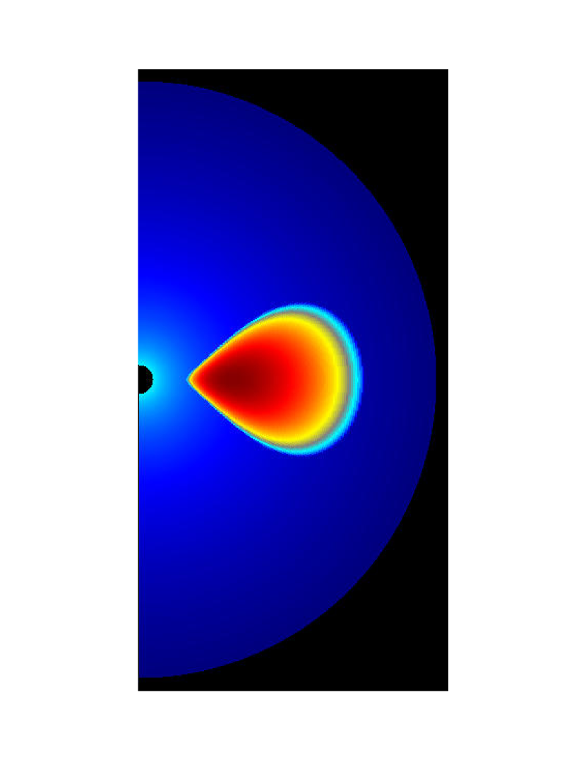
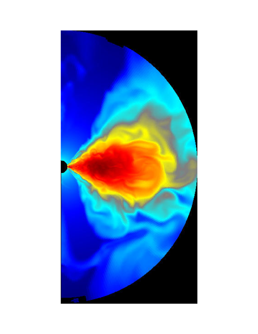
Figure 16: Density field, for a magnetized torus around a Kerr black hole with $a/M=0.5$ at $t=0$ (left) and at $t=2000M$ (right). The color is mapped from the logarithm of the density; black is low and dark red is high. The resolution is $300^{2}$.

The integration extends for $\Delta t=2000$, or about $7.6$ orbital periods at the pressure maximum. Figure 16 shows the initial and final density states projected on the $R=r\sin(\theta)$, $Z=r\cos(\theta)$ plane. Color represents $\log(\rho)$. The coordinate parameter $h$, which concentrates zones toward the midplane, is set to $0.2$. The torus atmosphere is set to the floor values (see above), and the MC limiter is used. The numerical resolution is $300^{2}$.

The flux of mass, energy, and angular momentum through the inner boundary are described in Figure 17. Initially the fluxes are small because the initial conditions are near an (unstable) equilibrium. The magnetorotational instability (Balbus & Hawley, 1991) e-folds for just over an orbital period, after which the magnetic field has reached sufficient strength to distort the original torus and drop material into the black hole. Later, the torus is turbulent and accretion occurs at a more or less steady rate.

6 Conclusion

Like all hydrodynamics codes, HARM has failure modes. We will discuss one that is likely to be relevant to future astrophysical simulations. When $B^{2}/\rho\gg 1$ and $B^{2}\gg u$, the magnetic energy is the dominant term in the total energy equation. Because the fields are evolved separately, truncation error in the field evolution can lead to large fractional errors in the velocity and internal energy. An example of this was discussed in §4.6, where the magnetized Bondi flow test fails for large values of $B^{2}/\rho$.

Another example can be found in the strong cylindrical explosion problem of Komissarov (1999), where an overpressured region embedded in a uniform magnetic field produces a relativistic blast wave. HARM fails on the strong-field version of this problem unless we turn the Courant number down to $0.1$, use the minmod limiter, and sharply increase the accuracy parameter used in the ${\bf P}({\bf U})$ inverter. This is a particularly difficult problem, with $B^{2}/\rho$ as large as $10^{4}$. The problems caused by magnetically dominated regions appears to be generic to conservative relativistic MHD schemes, where small errors in magnetic energy density lead to fractionally large errors in other components of the total energy. At present this is unavoidable, and has motivated the development of schemes for the evolution of the electromagnetic field in the force-free limit (Komissarov, 2002b).

Finally, to sum up: we have described and tested a code that evolves the equations of general relativistic magnetohydrodynamics. This code, together with the code described in a companion paper by de Villiers & Hawley (2002), are the first that stably evolve a relativistic plasma in a Kerr spacetime for many light crossing times. The advent of practical, stable GRMHD codes opens the door for the study of many problems in the theory of RMRs. For example, it may be possible to directly evaluate the importance of magnetic energy extraction from rotating black holes and the importance of black hole spin in determining jet parameters. It may also be possible to couple these schemes to numerical relativity codes and use them to study dynamical spacetimes with electromagnetic sources.

Figure 1: The ${\mathcal{L}}_{1}$ norm of the error in $u$ for a slow wave as a function of $N_{x}$ for both the monotonized central (MC) and minmod limiter. The straight lines show the slope expected for second order convergence.

Figure 2: The ${\mathcal{L}}_{1}$ norm of the error in the single nonzero component of the velocity for an Alfvén wave as a function of $N_{x}$ for both the monotonized central (MC) and minmod limiter. The straight lines show the slope expected for second order convergence.

Figure 3: The ${\mathcal{L}}_{1}$ norm of the error in $u$ for a fast wave as a function of $N_{x}$ for both the monotonized central (MC) and minmod limiter. The straight lines show the slope expected for second order convergence.

Figure 4: The run of density in the Komissarov nonlinear wave tests.

Figure 5: The run of $u^{x}$ in the Komissarov nonlinear wave tests.

Figure 8: Convergence results for the transport test.

Figure 9: A cut through the density in the nonrelativistic Orszag-Tang vortex solution from HARM (solid line, with $c=100$), from VAC (dashed line), and $4\times$ the difference (lower solid line) at a resolution of $640^{2}$.

Figure 10: Comparison of results from HARM and the nonrelativistic MHD code VAC for the Orszag-Tang vortex. The plot shows the ${\mathcal{L}}_{1}$ norm of the difference between the two results as a function of resolution for the primitive variables $\rho$ (squares) and $u$ (triangles). The straight line shows the slope expected for first order convergence. The errors are large because they are an integral over an area of $(2\pi)^{2}$.

Figure 11: Convergence results for the unmagnetized Bondi accretion test onto a Schwarzschild black hole. The straight line shows the slope expected for second order convergence.

Figure 12: Convergence results for the magnetized Bondi accretion test onto a Schwarzschild black hole. The straight line shows the slope expected for second order convergence.

Figure 13: The equatorial inflow solution in the Kerr metric for $a/M=0.5$ and magnetization parameter $F_{\theta\phi}=0.5$. The panels show density, radial component of the four-velocity in Boyer-Lindquist coordinates (with the square showing the location of the fast point), the $\phi$ component of the four-velocity, and the toroidal magnetic field $B^{\phi}=F^{\phi t}$.

Figure 14: Convergence results for the magnetized inflow solution in a Kerr metric with $a/M=0.5$. Parameters for the initial, quasi-analytic solution are given in the text. The straight line shows the slope expected for second order convergence. The ${\mathcal{L}}_{1}$ error norm for each of the nontrivial variables are shown. The small deviation from second order convergence at high resolution is due to numerical errors in the quasi-analytic solution used to initialize the solution.

Figure 15: Convergence results for the Fishbone and Moncrief equilibrium disk around an $a/M=0.95$ black hole.

Figure 17: Evolution of the mass accretion rate (top), the specific energy of the accreted matter (middle), and the specific angular momentum of the accreted matter (bottom) for a black hole with $a/M=0.5$.

References

- Abramowicz, Jaroszinski, & Sikora (1978) Abramowicz, M., Jaroszinski, M., & Sikora, M. 1978, A&A, 63, 221
- Anile (1989) Anile, A.M. 1989, Relativistic Fluids and Magneto-fluids, (New York: Cambridge Univ. Press)
- Balbus & Hawley (1991) Balbus, S.A., & Hawley, J.F. 1991, ApJ, 376, 214
- Balbus & Hawley (1998) Balbus, S.A., & Hawley, J. H. 1998, Rev. Mod. Phys., 70, 1
- Balsara (2001) Balsara, D. 2001, ApJS, 132, 83
- Blandford & Znajek (1977) Blandford, R.D., & Znajek, R. 1977, MNRAS, 179, 433
- Brio & Wu (1988) Brio, M., & Wu, C.C. 1988, JCP, 75, 500
- Del Zanna & Bucciantini (2002) Del Zanna, L., & Bucciantini, N. 2002, A&A, 390, 1177
- Del Zanna et al. (2002) Del Zanna, L., Bucciantini, N., & Londrillo, P., 2002, astro-ph/0210618
- Evans & Hawley (1988) Evans, C.R., & Hawley, J.F. 1988, ApJ, 332, 659
- Fishbone & Moncrief (1976) Fishbone, L.G., & Moncrief, V. 1976, ApJ, 207, 962
- Font (2000) Font, J. A. 2000, Liv. Rev. Rel., 3, 2000-2font
- Gammie (1999) Gammie, C.F. 1999, ApJ, 522, L57
- Harten et al. (1983) Harten, A., Lax, P.D., & van Leer, B. 1983, SIAM Rev. 25, 35
- Hawley, Smarr, & Wilson (1984) Hawley, J.F., Smarr, L.L., & Wilson, J.R. 1984, ApJS, 55, 211
- Koide et al. (2002) Koide, S., Shibata, K., Kudoh, T., & Meier, D.L. 2002, Science, 195, 1688
- Koide et al. (2000) Koide, S., Meier, D.L., Shibata, K., & Kudoh, T. 2000, ApJ, VVV, 668
- Koide, Shibata, & Kudoh (1999) Koide, S., Shibata, K., & Kudoh, T. 1999, ApJ, 522, 727
- Koldoba et al. (2002) Koldoba, A.V., Kuznetsov, O.A., & Ustyugova, G.V. 2002, MNRAS, 333, 932
- Komissarov (1999) Komissarov, S.S. 1999, MNRAS, 303, 343
- Komissarov (2001) Komissarov, S.S. 2001, in Godunov Methods: Theory and Applications, ed E.F.Toro, (New York: Kluwer) 519
- Komissarov (2002a) Komissarov, S.S. 2002, astro-ph/0209213
- Komissarov (2002b) Komissarov, S.S. 2002, MNRAS, 336, 759
- Lax & Wendroff (1960) Lax, P.D., & Wendroff, B. 1960, Comm. Pure App. Math, 13, 217
- LeVeque (1998) LeVeque, R.J. 1998, in Computational Methods for Astrophysical Fluid Flow (Berlin: Springer-Verlag) 1
- Marder (1987) Marder, B. 1987, JCP, 68, 48
- Martí & Muller (1999) Martí, J.M., & Müller, E. 1999, Liv. Rev. in Rel., 2, 1999-3marti
- Meier, Koide, & Uchida (2001) Meier, D.L., Koide, S., & Uchida, Y. 2001, Science, 291, 84
- Misner, Thorne, & Wheeler (1973) Misner, C., Thorne, K., & Wheeler J. 1973, Gravitation, (New York: Freeman) (MTW)
- Norman & Winkler (1986) Norman, M.L., & Winkler, K.-H. 1986, in Astrophysical Radiation Hydrodynamics, eds. K.-H. Winkler & M. Norman (Dordrecht: Kluwer), 449
- Orszag & Tang (1979) Orszag, S., & Tang, C.M. 1979, JFM, 90, 129
- Phinney (1983) Phinney, E.S., 1983, unpublished Ph.D. thesis, Cambridge University
- Punsly (2001) Punsly, B. 2000, Black Hole Gravitohydromagnetics, (New York: Springer)
- Van Putten (1993) Van Putten, M.H.P.M. 1993, JCP, 105, 339
- Ryu & Jones (1995) Ryu, D. & Jones, T.W. 1995, ApJ, 442, 228 (RJ)
- Shapiro & Teukolsky (1983) Shapiro, S.L., & Teukolsky, S.A. 1983, Black Holes, White Dwarfs, and Neutron Stars: The Physics of Compact Objects (New York: Wiley)
- Stone & Norman (1992) Stone, J.M., & Norman, M. 1992, ApJS, 80, 791
- Takahashi et al. (1990) Takahashi, M. , Nitta, S. , Tatematsu, Y. & Tomimatsu, A. 1990, ApJ, 363, 206
- Tóth (1996) Tóth, G. 1996, Astrophys. Lett. & Comm. 34, 245
- Tóth (2000) Tóth, G. 2000, JCP, 161, 605
- de Villiers & Hawley (2002) de Villiers, J.-P., & Hawley, J.F. 2002, ApJ, in press
- Wilson (1977) Wilson, J.R. 1977, in Proc. of the First Marcel Grossman Meeting on General Relativity, ed. R. Ruffini, (Amsterdam: North-Holland), 393
- Yokosawa (1993) Yokosawa, M. 1993, PASJ, 45, 207