Does the fine-structure constant vary with cosmological epoch?

Abstract

We use the strong nebular emission lines of O iii, 5007 Å and 4959 Å, to set a robust upper limit on the time dependence of the fine structure constant. We find $|\alpha^{-1}d\,\alpha(t)/dt|~{}<~{}2\times 10^{-13}$ yr^-1, corresponding to $\Delta\alpha/{\alpha(0)}~{}=~{}\left(0.7\pm 1.4\right)\times 10^{-4}$ for quasars with $0.16<z<0.80$ obtained from the SDSS Early Data Release. Using a blind analysis, we show that the upper limit given here is invariant with respect to 17 different ways of selecting the sample and analyzing the data. As a by-product, we show that the ratio of transition probabilities corresponding to the 5007 Å and 4959 Å  lines is $2.99\pm 0.02$, in good agreement with (but more accurate than) theoretical estimates. We compare and contrast the O iii emission line method used here with the Many-Multiplet method that was used recently to suggest evidence for a time-dependent $\alpha$. In an Appendix, we analyze the quasars from the recently available SDSS Data Release One sample and find $\Delta\alpha/{\alpha(0)}~{}=~{}\left(1.2\pm 0.7\right)\times 10^{-4}$.

1 Introduction

We develop in this paper a robust analysis strategy for using the fine-structure splitting of the O iii emission lines of distant quasars or galaxies to test whether the fine-structure constant, $\alpha$, depends upon cosmic time. We concentrate here on the two strongest nebular emission lines of O iii, 5007 Å and 4959 Å, which were first used for this purpose by Bahcall & Salpeter (1965).

We begin this introduction with a brief history of astronomical studies of the time dependence of the fine structure constant (§ 1.1) and then describe some of the relative advantages of using either absorption lines or emission lines for this purpose (§ 1.2). Next, we provide an outline of the paper (§ 1.3). Finally, since some of the material in this paper is intended for experts, we provide suggestions as to how the paper should be read, or not read (§ 1.4).

We limit the discussion in this paper to tests in which $\alpha$ is the only dimensionless fundamental constant whose time (or space) dependence can affect the measurements of quasar spectra in any significant way. For simplicity, we describe our results as if $\alpha$ could only change in time, not in space. However, our experimental results may be interpreted as placing constraints on the variation of coupling constants in the context of a more general theoretical framework.

1.1 A brief history

Savedoff (1956) set the first astronomical upper limit on the time dependence of $\alpha$ using the fine-structure splitting of emission lines of N ii and Ne iii in the spectrum of the nearby radio galaxy Cygnus A. He reported $\alpha^{2}(z=0.057)/\alpha^{2}(0)~{}=~{}1.0036\pm 0.003$. This technique was first applied to distant quasar spectra by Bahcall & Salpeter (1965), who used emission lines of O iii and Ne iii in the spectra of 3C 47 and 3C 147 to set an upper limit of $|\alpha^{-1}d\,\alpha(t)/dt|~{}<~{}10^{-12}$ yr^-1. Bahcall & Schmidt (1967) obtained a similar limit, $<~{}10^{-12}$ yr^-1, using the O iii emission lines in five radio galaxies. Here, and elsewhere in the paper, we shall compare limits on the time-dependence of $\alpha$ obtained at different cosmic epochs by assuming $\alpha$ depends linearly on cosmic time for redshifts less than five. The assumption of linearity may misrepresent the actual time dependence, if any, but it provides a simple way of comparing measurements at different redshifts.

The technique of using emission lines to investigate the time dependence of $\alpha$ was abandoned after 1967. In this sense, the present paper is an attempt to push the frontiers of the subject backwards three and a half decades.

Bahcall, Sargent, & Schmidt (1967) first used quasar absorption (not emission) lines to investigate the time dependence of $\alpha$. They used the doublet fine-structure splitting of Si ii and Si iv absorption lines in the spectrum of the bright radio quasar 3C 191, $z~{}=~{}1.95$. Although the results referred to a relatively large redshift, the precision obtained, $\alpha(z=1.95)/\alpha(0)~{}=~{}0.98\pm 0.05$, corresponding to $|\alpha^{-1}d\,\alpha(t)/dt|~{}<~{}7\times 10^{-12}$ yr^-1, did not represent an improvement.

Since 1967, there have been many important studies of the cosmic time-dependence of $\alpha$ using quasar absorption lines. Some of the most comprehensive and detailed investigations are described in papers by Wolfe, Brown, & Roberts (1976), Levshakov (1994), Potekhin & Varshalovich (1994), Cowie & Songaila (1995), and Ivanchik, Potekhin, & Varshalovich (1999). The results reported in all of these papers are consistent with a fine-structure constant that does not vary with cosmological epoch.

Recently, the subject has become of great interest for both physicists and astronomers because of the suggestion that a significant time-dependence has been found using absorption lines from many different multiplets in different ions, the ‘Many-Multiplet’ method (see, e.g., the important papers by Dzuba, Flambaum, & Webb 1999a,b; Webb et al. 1999; Murphy et al. 2001a,b; and Webb et al. 2002). The suggestion that $\alpha$ may be time dependent is particularly of interest to physicists in connection with the possibility that time-dependent coupling constants may be related to large extra dimensions (see Marciano 1984). Unlike the previous emission line or absorption line studies, the Many-Multiplet collaboration uses absolute laboratory wavelengths rather than the ratio of fine-structure splittings to average wavelengths. We shall compare and contrast in § 8 the emission line technique used here with the Many-Multiplet method.

1.2 Absorption versus emission lines

Why have absorption line studies of the time-dependence of $\alpha$ dominated over emission line studies in the last three and a half years? There are two principal reasons that absorption lines have been preferred. First, the resonant atomic absorption lines can be observed at large redshifts since their rest wavelengths fall in the ultraviolet. By contrast, emission line studies are limited to smaller redshifts ($z<1.5$) since the most useful emission lines are in the visual region of the spectrum. Second, there are many absorption lines, often hundreds, observed in the spectra of large redshift quasars and galaxies. These lines are produced by gas clouds at many different redshifts. There is only one set of emission lines with one redshift, representing the cosmic distance of the source from us, for each quasar or galaxy.

Why have we chosen to return to quasar emission lines as a tool for studying the time dependence of $\alpha$? We shall show that emission lines can be used to make precision measurements of the time dependence of $\alpha$ while avoiding some of the complications and systematic uncertainties that affect absorption line measurements. In addition, the large sample of distant objects made available by modern redshift surveys like the SDSS survey (Stoughton et al. 2002; Schneider et al. 2002) and the 2dF survey (Boyle et al. 2000; Croom et al. 2001) provide large samples of high signal-to-noise spectra of distant objects.

In this paper, we select algorithmically, from among 3814 quasar spectra in the SDSS Early Data Release (EDR, Schneider et al. 2002), the quasar spectra containing O iii emission lines that are most suitable for precision measurements. A total of 95 quasar spectra pass at least 3 out of the 4 selection tests we impose on our standard sample in § 5. Our Standard Sample contains spectra of 42 quasars. We also study alternative samples obtained using variants of our standard selection algorithm. These alternative samples contain between 28 and 70 individual quasar spectra.

The techniques described in this paper could be applied to similar transitions in [Ne iii] ($\lambda\lambda~{}3968,3869$) and in [Ne v] ($\lambda\lambda~{}3426,3346$). However, the [O iii] emission lines are typically an order of magnitude stronger in quasar spectra than the just-mentioned transitions of [Ne iii] and [Ne v] (cf. Vanden Berk et al 2001; Schneider et al. 2002). Moreover, the intensity ratio of the [O iii] lines is a convenient value (about 3.0) and the relevant region of the spectrum is relatively free of other possibly contaminating emission or absorption lines. After [O iii], the [Ne iii] lines are the most promising pair of emission lines for studies of the time dependence of $\alpha$.

1.3 Outline of the paper

We present in § 2 a summary of the main ingredients in the analysis we perform. Then in § 3 we describe how we developed the selection algorithm and performed the analysis blindly, i.e., without knowing what the results meant quantitatively until all of the measurements and calculations were complete. We present in § 4 the key procedure which we have used to measure by how many Angstroms we have to shift the observed 4959 Å line profile to obtain a best-fit match to the 5007 Å line profile.

The Standard Sample of quasar spectra that we measure is selected objectively by applying four computer tests designed to ensure that emission line pairs that are used in the analysis will yield accurate and unbiased estimates of $\alpha$. These selection tests are described in § 5. Figure 4 illustrates a good quasar spectrum that easily passes all of the computer tests. Figure 5 shows four spectra, each of which illustrates a failure to satisfy one of the four standard tests.

Table 1 and Table 2, together with Figure 7, present our principal results The results for our Standard Sample are explained in § 6, where we discuss the average value of $\alpha$ and the best-fit slope, $d\alpha(t)/dt$, for our Standard Sample of 42 quasars. We also describe in this section the bootstrap method that we have used to calculate the uncertainties for the sample characteristics. In § 7, we describe and discuss the analysis of 17 additional samples chosen by alternative selection algorithms. We describe the ‘Many-Multiplet’ method in § 8 and contrast the O iii method with the Many-Multiplet method. We summarize and discuss our results for the SDSS Early Data Release Sample in § 9.

Note added in proof. Since this paper was written, many more quasar spectra have become available from the SDSS Data Release One sample (see Schneider et al. 2003). We have analyzed this much larger sample of quasars using exactly the same technique as described in the main body of the present paper. We present our results for the SDSS Data Release One sample in Appendix C.

1.4 How should this paper be read?

This paper contains many different things, including (not necessarily in this order): 1) a detailed discussion of the algorithmic basis for selecting the 18 different samples that we analyze, 2) a description of how our algorithmic measurements are made in practice, 3) a discussion of the errors in the measurements, 4) tabulated details of the measurements sufficient to allow the reader to change or check the data analysis, 5) quantitative results on the time dependence of the fine structure constant in our Standard Sample, 6) quantitative results on the time dependence of $\alpha$ for 17 alternative samples, 7) a comparison of the Many-Multiplet and O iii methods for studying the time dependence of the fine structure, and 8) a summary and discussion of our main conclusions. In addition, we present an accurate measurement of the ratio of the two forbidden transition probabilities that lead to the 5007 Å and 4959 Å lines.

Most readers will only want to sample part of this fare. Here is our suggestion as to how to get the most out of the paper in the shortest amount of time. We assume that you have read the introduction. If so, then you probably will want to first read § 2, which gives an outline of the procedure we follow, and then look at Figure 1, Figure 4, and Figure 7. Next read the conclusions and discussion in § 9. If you are especially interested in the differences between the O iii method and the Many-Multiplet method, then look at Table 3 and, if you want more details about the differences, read § 8. Our principal quantitative results are given in § 6 and § 7. Unless you are an expert, you can skip everything in § 6 and § 7 except the simple equations that give the main numerical results: equation (17)–equation (24). Sections 3–5 contain the main technical discussion of this paper. These sections are essential for the expert who wants to decide whether we have done a good job. But, if you have already made up your mind on this question, you can skip §§ 3–5.

2 Outline of measurement procedure

Figure 1: Energy level diagram for O iii. The figure shows the two strong emission lines that arise from the same ${}^{1}D_{2}$ excited level of twice-ionized oxygen. The $5007$ Å  and $4959$ Å  lines are separated by about $48$ Å by the fine-structure energies of the ground-state triplet P states. The wavelength separation $\Delta\lambda$ divided by the sum of the wavelengths of the two emission lines is proportional to $\alpha^{2}$; this dimensional-less ratio (difference divided by sum)is defined as $R$ in equation (1). The quantity $R$ can be measured in distant quasars or galaxies and is independent of cosmological epoch unless $\alpha^{2}$ depends upon time.

Figure 1 shows the relevant part of the energy level diagram for twice-ionized oxygen, O iii. We utilize in this paper the two strongest nebular emission lines of [O iii], $\lambda 5007$ and $\lambda 4959$, both of which originate on the same initial excited level, ${}^{1}D_{2}$. Since both lines originate on the same energy level and both lines have a negligible optical depth (the transitions are strongly forbidden), both lines have exactly the same emission line profile. If there are multiple clouds that contribute to the observed emission line, then the observed emission line profiles are composed of the same mixture of individual cloud complexes.

The two final states are separated by the fine-structure interaction. Thus the energy separation of the $\lambda 5007$ and $\lambda 4959$ emission lines is proportional to $\alpha^{4}$, while the leading term in the energy separation for each line is proportional to $\alpha^{2}$. To very high accuracy (see § A of the Appendix,), the difference in the wavelengths divided by the average of the wavelengths, R,

$$R(t)~{}=~{}\frac{\lambda_{2}(t)-\lambda_{1}(t)}{\lambda_{1}(t)+\lambda_{2}(t)}\,,$$ (1)

is proportional to $\alpha^{2}$. The cosmological redshift of the astronomical source that emitted the oxygen lines cancels out of the expression for $R$, which depends only on the ratio of measured wavelengths, either added or subtracted. Thus a measurement of $R$ is a measurement of $\alpha^{2}$ at the epoch at which the [O iii] lines are emitted. The key element in measuring $R(t)$ is the determination of the shift in Angstroms that produces the best-fit between the line profiles of the two emission lines.

The wavelengths in air of the nebular emission lines

$$\lambda_{1}~{}=~{}4958.9110~{}\mbox{\AA};~{}~{}~{}~{}~{}\lambda_{2}~{}=~{}5006.8430~{}\mbox{\AA},$$ (2)

and their separation

$$\Delta\lambda~{}=~{}47.9320~{}\mbox{\AA}.,$$ (3)

have been measured accurately from a combination of laboratory measurements with a theta-pinch discharge (Pettersson 1982) and, for the wavelength separation, infrared spectroscopy with a balloon borne Michelson interferometer (Moorwood et al. 1980). The conversion from vacuum wavelengths to wavelengths in air was made using the three term formula of Peck and Reeder (1972). Combining equation (2) and equation (3), we have

$$R(0)~{}=~{}4.80967\times 10^{-3}\left[1\pm 0.00001\right]\,,$$ (4)

where the error for $R(0)$ is based primarily on measurement by Moorwood et al. (1980) of the intervals in the ground ${}^{3}P$ multiplet (see also Pettersson 1982).

One can write the ratio of $\alpha^{2}$ at much earlier time $t$ to the value of $\alpha^{2}$ obtaining at the current cosmological epoch as

$$\frac{R(t)}{R(0)}~{}=~{}\frac{\alpha^{2}(t)}{\alpha^{2}(0)}~{}=~{}\left[\frac{\Delta\lambda(t)}{\lambda_{1}(t)+\lambda_{2}(t)}\right]\left[\frac{\lambda_{1}(0)+\lambda_{2}(0)}{\Delta\lambda(0)}\right].$$ (5)

The light we observe today was emitted by distant quasars (or galaxies) at an epoch that was $10^{9}$ yr or $10^{10}$ yr earlier. This huge time difference makes possible precise measurements of the time dependence of $\alpha^{2}$ by recording the redshifted wavelengths of the [O iii] emission lines emitted at a much earlier epoch.

We will compare values of R, i.e., $\alpha^{2}$, measured at different cosmological epochs. Although the data are consistent with a time-independent value for $\alpha^{2}$, we will find an upper limit to the possible time-dependence by fitting the measured values of $R(t)$ to a linear function of time,

$$R(t)~{}=~{}R(0)[1+StH_{0}].$$ (6)

Here $R(t)$ is a function of $z$, $R(t(z))$, where $z$ is the cosmological redshift [see eq. (8)] below for the relation between $t$ and $z$). The slope $S$ is twice the logarithmic derivative of $\alpha^{2}(t)$ with respect to time in units of one over the Hubble constant.

$$S~{}=~{}\frac{1}{H_{0}\alpha^{2}}\left(\frac{d\alpha^{2}}{dt}\right)~{}=~{}\frac{2}{H_{0}\alpha}\left(\frac{d\alpha}{dt}\right)$$ (7)

As defined in equation (6) and equation (7), the slope S is independent of $H_{0}$. Each redshift produces a unique value of $H_{0}t$.

We do not need to know $\alpha^{2}(0)$, or equivalently, $\lambda_{1}$ and $\lambda_{2}$ (or $R(0))$, in order to test for the time dependence of $\alpha$. We can use equation (5) and equation (6) to explore the time dependence by simply taking taking $\alpha^{2}(0)$ to be any convenient constant. In fact, this is exactly what we have done, which enabled us to carry out a blind analysis (see discussion in § 3). For 16 of the 17 samples we have analyzed, we have not made use of the known local value for $R(0)$, i.e., $\alpha^{2}(0)$ (see § 7).

The cosmological time can be evaluated from the well known expression (e.g., Carroll and Press 1992)

$$t=\frac{t_{0}-t_{1}}{H_{0}}=\int_{0}^{z}\frac{dz}{(1+z){\sqrt{(1+z)(1+\Omega_{m}z)-z(2+z)\Omega_{\Lambda}}}}\,,$$ (8)

where $\Omega_{m}$ and $\Omega_{\Lambda}$ are the usual present-epoch fractional contributions of matter and a cosmological constant to the cosmological expansion. The translation between the Hubble constant, $H_{0}$, and a year is given by

$$\frac{1}{H_{0}}~{}=~{}1.358\times 10^{10}{\rm~{}yr^{-1}}\left(\frac{72~{}{\rm km\,s^{-1}Mpc^{-1}}}{H_{0}}\right).$$ (9)

In what follows, we shall adopt the value for $H_{0}$ determined by the HST Key Project, i.e., $H_{0}=72~{}{\rm km\,s^{-1}Mpc^{-1}}$ (Freedman et al. 2001). If the reader prefers a different value for $H_{0}$, all times given in this paper can be rescaled using equation (9). Except where explicitly stated otherwise in the remainder of the paper, the time $t$ is calculated from equation (8) and equation (9) for a universe with the present composition of $\Omega_{m}=0.3,\,\,\Omega_{\Lambda}=0.7$.

3 Blind analysis

To avoid biases, we performed a blind analysis.

Measurements of $\alpha^{2}$ were computed relative to an artificial value of $\alpha^{2}(0)_{\rm artificial}=1.0$. We did not renormalize the measured values of $\alpha^{2}(t)$ until the analysis was complete. In fact, we did not search out the precise values of the wavelengths given in equation (2) until after we had finished all our calculations of $\alpha^{2}(t)$ from the measured wavelengths. Throughout all the stages when we were determining the selection criteria for the sample described in § 5, we worked with measured values for $\alpha^{2}(t)$ that were about 0.0048 [cf. eq. (4)]. At this stage, we had not researched the precise values of the local wavelengths for the [O iii] emission lines. Therefore, we did not know whether the measured values that we were getting for $\alpha^{2}(t)$ were close to the local value and, if so, how close.

To further separate the measuring process from any knowledge of the local value for $\alpha(0)$, we developed the criteria for selecting the sample using a subset of the quasars in the SDSS EDR sample. We used in this initial sample 313 quasars with redshifts $z<0.80$. After finalizing the selection criteria, we applied the criteria to the remaining 389 quasars with $z<0.80$ in the EDR. The acceptance rate for the initial sample was 23 objects out of 313 or $7.7$%, while the acceptance rate for the second sample was 19 out of 389 or $5.1$%. We will refer later to the combined sample of 42 objects selected in this way as our ‘standard sample.’

The estimates of $\alpha^{2}$ derived for the two parts of the standard sample were in excellent agreement with each other. For the initial sample of 23 objects, we found

$$\left<\alpha^{2}\right>~{}=~{}1.0002\pm 0.0004\,,$$ (10)

and for the second sample of 19 objects we found

$$\left<\alpha^{2}\right>~{}=~{}1.0001\pm 0.0004\,.$$ (11)

The sample average for the 42 objects is $1.0001\pm 0.0003$ (cf. row one of Table 1 in § 6).

4 Matching the 5007 Å and 4959 Å line shapes

The key element in our measurement of $\alpha$ is the procedure by which we match the shapes of the 5007 Å and 4959 Å emission line profiles. What we want to know is by how many Angstroms do we have to shift the 4959 Å line so that it best fits the measured profile of the 5007 Å line. In the process, we also determine a best-estimate for the ratio of the intensities in the two lines.

Figure 1 shows that both of the emission lines, [O iii] 5007 Å and 4959 Å, arise from the same initial atomic state. Hence both lines have (within the accuracy of the noise in the measurements) the same line profile, i.e., the same shape of the curve showing the flux intensity versus wavelength, although the two lines are displaced in wavelength and have different intensities.

We have developed a computer code, FitAlpha, that finds the best match of the shapes of the 5007 Å and 4959 Å lines in terms of two parameters, $\eta$ and $A$. The two parameters describe how much the measured profile of the 4959 Å line must be shifted in wavelength, $\eta$, and how much the 4959 Å profile must be increased in amplitude, $A$, in order to provide the best possible match to the profile of the 5007 Å emission line.

We first discuss in § 4.1 the measurements of the amplitude ratios $A$ and then describe in § 4.2 the measurements of the quantity that describes the wavelength shift, $\eta$. We show in § 4.3 that the measured values of $A$ and $\eta$ are not significantly correlated. We conclude by describing in § 4.4 the errors that we assign to individual measurements of $\alpha^{2}$.

4.1 Amplitude ratios A

In the limit in which the profiles of the 5007 Å and 4959 Å lines match identically and there is no measurement noise, the quantity $A$ is the ratio of the area under the 5007 Å line to the area under the 4959 Å line. More explicitly, in the limit of an ideal match of the two line profiles,

$$A~{}=~{}\frac{\int_{5007}\left[{\rm LineFlux(\lambda)-ContinuumFlux(\lambda)}\right]d\lambda}{\int_{4959}\left[{\rm LineFlux(\lambda)-ContinuumFlux(\lambda)}\right]d\lambda}\,.$$ (12)

In practice, the best-fit ratio of the amplitudes, which is measured by FitAlpha, is better determined than the area under the emission lines. Thus, the values we report for $A$ (e.g. in Table 4 in § B of the Appendix) are the best-fit ratios of the amplitudes. Although $A$ is one of the outputs of FitAlpha, we do not make use of $A$ except as a post facto sanity check that the fits are sensible.

Figure 2: The ratio of amplitudes, $A$. The figure shows a histogram for our standard sample of quasars of the ratio $A$, which is the best-fit ratio of the amplitude of the 5007 Å profile to the amplitude of the 4959 Å profile. The measured average value of $A$ is in good agreement with the expectation based upon the tabulated data in the NIST Atomic Spectra Database [see eq. (13) and eq. (14) and related text].

Figure 2 presents a histogram of the values of A that were measured for quasars in our standard sample, which is defined in § 5. Our measurements have a typical $1\sigma$ spread of about $\pm 0.1$. The sample average of the measurements for A, and the bootstrap uncertainty determined as described in § 6.2, are

$$\left<A_{\rm measured}\right>~{}=~{}2.99\pm 0.02\,.$$ (13)

The quantity $\left<A_{\rm measured}\right>$ is equal to the ratio of the decay rates of the 5007 Å and the 4959 Å lines, i.e., the ratio of the Einstein A coefficients. Thus the measured value for the ratio of the transition probabilities corresponding to the 5007 Å and 4959 Å lines is

$$\frac{A\left(5007\right)}{A\left(4959\right)}~{}=~{}2.99\pm 0.02\,.$$ (14)

The measured value of ${A\left(5007\right)}/{A\left(4959\right)}$ is consistent with the best theoretical estimate given in the NIST Atomic Spectra Database, ${A\left(5007\right)}/{A\left(4959\right)}=2.92$ (Wiese, Fuhr, and Deter 1996). The quoted NIST accuracy level for this theoretical estimate is ‘B’, which generally corresponds to a numerical accuracy of better than 10%. Our measurement is more accurate than the theoretical estimate.

4.2 Measuring $\eta$ and R

We define $\eta$ by the relation

$$\eta~{}\equiv~{}\frac{\lambda_{2}}{\lambda_{1}}-1,$$ (15)

where $\lambda_{1}$ and $\lambda_{2}$ are the measured values of the redshifted emission lines corresponding to the lines with rest wavelengths given by equation (2). We use the measured values of $\eta$ to calculate the value of $\alpha^{2}(z)$ for each source. The ratio R defined by equation (1) can be written in terms of $\eta$ as

$$R~{}=~{}\frac{\eta}{\eta+2}.$$ (16)

FitAlpha finds the best-fit values of $\eta$ as follows. The Princeton 1-D reduction code (Schlegel 2003) determines the redshift of the quasar by fitting the entire quasar spectrum to a template. This fit yields an approximate value for the redshift that locates the 4959 Å and 5007 Å lines to within 2-3 spectral pixels. Each of the spline-resampled pixels has a width of $69.0{\rm\,km\,s^{-1}}$. FitAlpha selects a 20 pixel wide region of the spectrum centered around the expected center of the 4959 Å line and a wider (35 pixel) region around the expected center of the 5007 Å line. The Spectro-2D code represents each quasar spectrum as a $4^{\rm th}$ order B-spline, where the spline points are spaced linearly in log-wavelength (Burles & Schlegel 2003), $\log\lambda_{1}={\rm const.}+10^{-4}\times i$. The optical output of the SDSS spectrograph gives pixel elements that are very nearly proportional to $\log\lambda$. This B-spline can be evaluated at any choice of wavelengths. We chose to evaluate each spectrum on a dense grid spaced in units of $10^{-5}$ in log-wavelength ($\sim 0.1$ pixel), corresponding to approximately 6.9${\rm~{}km\,s^{-1}}$. The measured average full width at half maximum of the 5007 Å lines in our standard sample is 5.5 pixels ($\sim 9$ Å).

The SDSS spectra cover the wavelength region 3800–9200 Å . The resolution (FWHM) varies from $140{~{}\rm to~{}}170\rm\,km\,s^{-1}$, with a pixel scale within several percent of $69{\rm\,km\,s^{-1}}$ everywhere (Burles & Schlegel 2003). The wavelength solution is performed as a simultaneous fit to an arc spectrum observation and the sky lines as measured in each object observation. The arc lines constrain the high-order terms in the wavelength calibration, while the sky lines constrain any small flexure terms and plate scale changes between the arc and object observations. The RMS in the recovered arc and sky line positions is measured to be approximately $1{\rm\,km\,s^{-1}}$. Therefore, it is possible that systematic errors could remain in the wavelength calibration at this level (Burles & Schlegel 2003). The flux-calibration has been shown to be accurate to a few percent on average, which is impressive for a fiber-fed spectrograph (Tremonti et al. 2003, in preparation). The remaining (small) flux-calibration residuals are coherent on scales of 500 Å , which has negligible effect on our line centers which are measured using regions $<100$ Å wide.

The measured profile of the 4959 Å line is compared with each of the spline-fit representations of the 5007 Å region. We make the comparison only within a region of $2\times 10^{-3}$ in log-wavelength (about 23 Å). For each possible shift between the two emission lines in log-wavelength, we minimize over the multiplicative scale factor $A$ between the profiles of the two lines and a quadratic representation of the local continuum. This continuum is primarily the approximately power-law of the quasar spectrum and the wings of the H$\beta$ line. The value of $\eta$ [cf. eq. (15)] is determined by minimizing the $\chi^{2}$ value for the fit between the two line shapes.

4.3 Are $\eta$ and A correlated?

It is natural to ask if the measured values of $\eta$ and A are correlated since they are both determined by the same computer program. A priori, one would not expect the two variables to be correlated if the best shift and the best rescaling are really disjoint. For the comparison of two lines with the same intrinsic shape, the shift and the rescaling should be independent of each other. However, computer programs that process real experimental data do not always yield the expected answer. Hence, we have checked whether there is a significant correlation between the observed values of $\eta$ and A.

Figure 3 shows all the measured values of (A,$\eta$) for all 42 quasars in our standard sample. The figure looks like a scatter diagram and indeed the computed linear correlation coefficient is only -0.034. If there were no intrinsic correlation between $\eta$ and A, one would expect just by chance to obtain a correlation coefficient bigger than the measured value in 83% of the cases. We conclude that there is no significant correlation between $\eta$ and A.

Figure 3: Lack of correlation between $\eta$ and A. The plotted points represent the measured values of A and $1000\times\eta$ for all 42 quasars in our standard sample.

4.4 Error estimates on individual measurements

The errors on the measured SDSS fluxes are not perfectly correct; the pipeline software overestimates the errors for lower flux levels. We correct the errors approximately by multiplying all of the errors by a constant factor (typically of order 0.75) chosen to make $\chi^{2}$ per degree of freedom equal to $1$ for the best-fit value of $\eta$. These adjusted errors are used to evaluate the uncertainty in the measured value of $\eta$. However, we show in § 6 and in § 7.2.4 that the bootstrap error for the sample average value of $\alpha$ and of the first derivative of $\alpha$ with time are very insensitive to the estimated uncertainties in the individual measurements.

The error on the measured value of $\alpha^{2}$ is dominated by the error on the measurement of the wavelength separation, $\Delta\lambda$, between the 5007 Å and the 4959 Å line. Before making the measurements, we estimated, based upon prior experience with CCD spectra, that we should be able to measure $\Delta\lambda$ to about 0.05 of a pixel. Since the width of each pixel is about 70 ${\rm km\,s^{-1}}$, or about 1.2 Å at 5000 Å, we expected to be able to make measurements of $\alpha^{2}$ that were accurate to about $1.2\times 10^{-3}$. As we shall see in § 6 (cf. Table 4 of § B of the Appendix), the average quoted error for an individual measurement of $\alpha^{2}$ is $1.8\times 10^{-3}$, somewhat larger (but not much larger) than our expected error.

5 Sample selection tests

We begin this section with some introductory remarks, made in § 5.1, about the sample and the sample selection. In the last four subsections of this section, §§ 5.2–5.5, we define four standard tests that were used to select the standard sample of quasar spectra from which we have determined our best estimates of $\alpha^{2}$ and $\alpha^{-2}d\alpha^{2}/dt$. Our standard sample, discussed in § 6, passes all four of the tests as described here. We present in § 7.1 a number of variations of the standard tests.

5.1 Introductory remarks about the spectra and the sample selection

5.1.1 Spectra used

We list in Table 5 of § B of the Appendix each of the 95 quasars in the SDSS EDR sample that have passed at least three of the four standard tests that we describe later in this section. Table 5 shows which of the four tests each quasar satisfies. The table also gives the measured value of $\eta$ [see eq. (15)] for every quasar that we have considered. If the reader would like to perform a different data analysis using our sample, this can easily be accomplished with the aid of Table 5, eqs. (1)–(7), and equation (16).

Although the spectra that we use here were obtained from the SDSS Early Data Release, the spectral reductions that we use are significantly improved over the reductions given in the EDR. Improvements in the reduction code are described in Burles and Schlegel (2003).

As described in § 3, the four standard tests were developed using an initial sample of 313 quasars in the EDR data of SDSS that could potentially show both of the [O iii] emission lines. The range of redshifts that was included in this initial sample is $z=0.163$ to $z=0.799$. The complete EDR sample of quasars that we have studied includes 702 quasars with redshifts ranging from $z=0.150$ to $0.799$. A total of 23 out of 313 quasars in our initial sample passed all four of the tests described below. In our final sample, 42 quasars passed all four tests. In what follows, we shall refer to the 23 accepted quasar spectra as our “initial sub-sample” and the 42 total accepted quasars as our “standard” sample.

Unfortunately, the majority of the EDR spectra that we examined were not suitable for measurement. In nearly all of these unsuitable spectra, the O iii lines did not stand out clearly above the continuum or above the noise. In a very few cases, we encountered a technical problem processing the spectra. As the first step in our ‘blind analysis’, before we imposed our four standard tests, we threw out unsuitable spectra by requiring that both of the O iii lines have a positive equivalent width and that the fractional error in $\alpha^{2}$, determined from equation (5), be less than unity. Only 260 out of the 702 quasar spectra (37%) in which the O iii lines could have been measured passed this preliminary filtering and were subjected to the standard four tests to determine the standard sample. Post facto, we checked that our results were essentially unchanged if we omitted this preliminary cut on unsuitable spectra, namely: the standard sample we analyze increased from 42 to 45 objects, the sample average of $\left<\alpha(z)\right>$ decreased by 0.002%, and the calculated error bar increased by 0.4%. We chose to impose the preliminary cut on suitable spectra because it increased our speed in analyzing a variety of alternative cuts discussed in § 7.

5.1.2 Standard cuts

The standard cuts described in the following subsections were imposed in the ‘blind’ phase of our analysis in order to make sure that the accepted spectra were of high quality and that the line shapes of the 5007 Å and 4959 Å lines were the same. Although we were seeking to eliminate any sources of biases by eliminating problematic spectra before we made the measurements, we have found post facto no evidence that omitting the any of the cuts would have led to a systematic bias.

We wanted to guard against contamination by H$\beta$ emission and to ensure that the signal to noise ratio was high. We also devised two tests that checked on the similarity of the two line shapes, the KS test discussed in § 5.2 and the line peak test described in § 5.3. In practice, all of these tests, with the exception of the check on H$\beta$ contamination, are designed to prevent noise fluctuations or unknown measuring errors from distorting the shape of one or both of the emission line profiles.

We shall see in § 7 that we could have been less stringent in imposing a priori criteria for acceptance of quasar spectra. We describe in § 7 the results that were obtained for four separate samples in which we omitted a different one of each of the four standard tests described in § 5.2–§ 5.5. We also present the results of analyses made using a variety of weaker versions of the four selection tests discussed in the present section. Although we obtain larger samples by using less stringent acceptance criteria, the final results for the time dependence of $\alpha$ are robust, essentially independent of the form and number of the selection tests. Essentially, we can trade off spectral quality versus number of accepted spectra without significantly changing the final conclusion.

Figure 4 shows the spectrum of SDSS 105151-005117, z = 0.359, which easily passes all of the selection criteria described below. If all of the quasar spectra were as clean and as well measured as the spectrum of SDSS 105151-005117, no selection tests would be required. We also show in the right hand panel of Figure 4 the continuous spline fit of the shape of the 5007 Å line that, when the center is shifted in wavelength and the amplitude of the curve is decreased by a constant factor ($A$), best-matches the measured data points for the 4959 Å line shape.

           

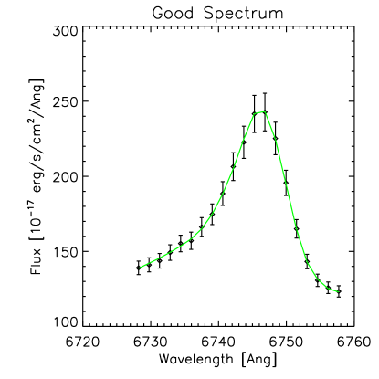
Figure 4: A good spectrum. The figure shows the spectrum of SDSS 105151-005117, which is also PG 1049-005. The quasar has a redshift of z = 0.359. The quasar spectrum easily passes all four of the tests described in § 5. The left panel shows the measured quasar energy spectrum in the wavelength region of interest. The approximately horizontal line near the zero flux level represents the estimated total error in the flux at each pixel. The right hand panel shows as a continuous curve the best-fit spline to the measured shape of the 5007 Å line, after shifting the line center ($\eta$), decreasing the amplitude ($A$), and super-imposing the spline fit on the measured data points of the 4959 Å line.

           

           

Figure 5: Examples of four failed spectra. The figure shows examples of spectra that failed each of the tests described in § 5. The spectrum in the upper left panel failed the KS test (cf. § 5.2); the upper right panel shows a spectrum in which the peaks failed to line up correctly (cf. § 5.3). The lower left panel displays a spectrum in which the H$\beta$ line is so large that it might contaminate the [O iii] 4959 Å (cf. § 5.4); the lower right panel shows a spectrum in which the signal to noise ratio is too low to permit an accurate measurement of the splitting between the two [O iii] emissions lines (cf. § 5.5) .

Figure 5 and Figure 6 illustrate the reasons why we need to impose selection criteria, or tests, to determine which quasar spectra can yield precise measurements of the wavelengths of the redshifted [O iii] lines. Figure 5 shows the measured spectrum shape for four different quasars and Figure 6shows, for the same four quasars, the best spline fits of the 5007 Å line shapes to the measured shape of the 4959 Å line. The various panels show spectra in which the measurements are compromised by different problems. In the upper left panels of Figure 5 and Figure 6, the [O iii] lines have somewhat different shapes and in the upper right panels the peaks of the two lines can not be lined up precisely by a linear shift in wavelengths. In the lower left panels, the H$\beta$ line is so strong that it might distort the profile of the 4959 Å line. The spectra in the lower right panels have too low a signal to noise ratio to allow a precise measurement.

In the following subsections, we shall define more quantitatively the criteria for passing these four tests. We have formulated the tests as computer algorithms that can be applied quickly and easily to numerical spectra.

We describe in § 5.2 the Kolmogorov-Smirnov test that we have applied to the emission line shapes in order to select acceptable quasar spectra. In § 5.3, we describe a test which requires that the peaks of the two emission lines essentially lie on top of each other when the line profiles are optimally shifted and rescaled. We present in § 5.4 a test that eliminates quasar spectra with a large H$\beta$ contamination of the 4959 Å line. Finally, we describe in § 5.5 a requirement that the area under the 5007 Å line be measured with a high signal-to-noise ratio. For brevity, it is convenient to refer to these tests as the KS, line peak, H$\beta$, and signal-to-noise criteria. In § 5.6, we show post facto that Fe ii lines do not compromise our measurements of $\alpha^{2}(t)$.

           

           

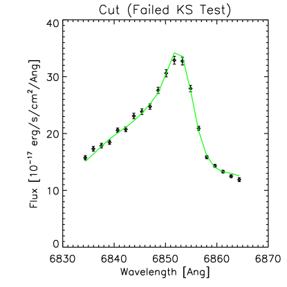
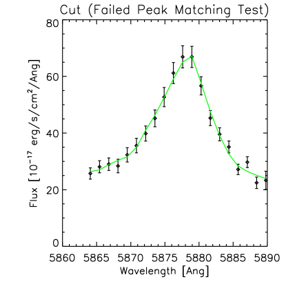
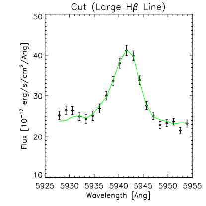
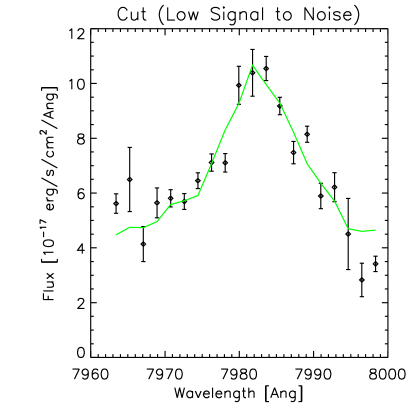
Figure 6: Examples of four failed fits. The quasar emission lines shown in this figure are the same as are shown in Figure 5. For each of the four examples of failed spectra shown in Figure 5, Figure 6 shows the corresponding best (but failed) spline fit of the measured shape of the 5007 Å line (continuous curve)to the measured shape (points with error bars) of the 4959 Å line.

5.2 Kolmogorov-Smirnov test

We represent the shapes of the emission line profiles by the seven measured flux values that are centered on the line peak. We then use a Kolmogorov-Smirnov (KS) test to determine whether the seven flux values centered on the peak of the 4959 Å line shape are, after multiplying by a constant factor $A$ [see eq. (12) and related discussion] consistent with being drawn from the same distribution as the seven flux values centered on peak of the 5007 Å line shape. The spectrum in the upper left hand panel of Figure 5 was rejected because the two [O iii] lines have slightly different shapes. For an unknown reason (which could be an instrumental or measuring error or simply a fluctuation), the 4959 Å line has a slight extra contribution on the short wavelength side of the line profile.

If the two line shapes are the same before being affected by noise and measuring errors, as required by the analysis described in § 4, then the two lines will generally pass a KS test. We set our level for acceptance such that there are only a few false negatives, i.e., spectra incorrectly rejected. In principle, there could be some false positives since the KS test does not require that the flux values match in wavelength as well as in intensity. In practice, false positives of this kind essentially never occur.

We require that the two sets of 7 flux values be drawn from the same distribution to a confidence level (C.L.) corresponding to $2\sigma$ (95% C.L.). From our initial sample of 313 quasars in the redshift range that allowed the observation of the [O iii] lines, 13 quasars failed this test but no other test. Five of the 13 quasars that failed the test had values of $\alpha^{2}$ that differed by at least $2\sigma$ from the sample average of $\alpha^{2}$. In the full EDR sample, 28 quasars failed only this test. Out of the 260 quasars that passed the preliminary spectral quality test described in § 5.1, only 80 passed the KS test. Out of the total sample of 702 objects with redshifts that permitted the measurement of the O iii lines, only 99 passed the KS test.

The requirement that the shapes of the 5007 Å and 4959 Å lines be similar according to the KS test is our most stringent test.

We show in § 7 that the results are essentially unchanged if we use the central 11 flux values instead of the central 7 values (see row four of Table 1 and Table 2) or if we omit the KS test entirely (see row eight of Table 1 and Table 2).

5.3 Lining up the peaks

We require that the peak of the 4959 Å line and the peak of the shifted 5007 Å line lie in the same pixel, for the best-fit value of $\eta$. The demand that the two peaks be lined up after the 4959 Å line is optimally shifted strengthens the constraint that the two shapes be the same. Since this test requires that the peaks line up but does not constrain the shift $\eta$, the test enforces the requirement that the shapes of the two lines be the same but does not constrain the possible values of $\alpha$. In principle, this test may occasionally reject otherwise acceptable spectra if the peak of one of the lines lies very near the boundary between two pixels. In the initial sample, only two quasars failed this test but no other test. Both of the quasars which failed were $2\sigma$ outliers. In the full EDR sample, eight quasars failed only this test. Out of the 260 quasars that passed the preliminary spectral quality test described in § 5.1, 152 passed the test of the lining up of the peaks. From the total sample of 702 objects with appropriate redshifts for measuring O iii lines, 247 passed the line peak test.

If we omit the line peak test, the sample size increases by nine objects, but the overall results are unchanged (see row nine of Table 1 and Table 2).

5.4 H$\beta$ contamination

The H$\beta$ line, which is centered at 4861 Å, can contaminate the 4959 Å line if H$\beta$ is too strong. Moreover, the presence of a strong H$\beta$ line could in principle distort the continuum fit. Therefore, we require that the area under the H$\beta$ line be no more than twice the area under the 5007 Å line. In practice, this requirement ensures that the contamination of the 4959 Å line from the H$\beta$ line is less than the contamination from the 5007 Å line. In our initial sample, three quasars failed only this test. In the full EDR sample, four quasars failed only this test. None of the quasars that failed this test were $2\sigma$ outliers. Out of the 260 (702) quasars that passed the preliminary spectral quality test (for which the quasar redshift permitted the measurement of the O iii lines), 231 (333) passed the H$\beta$ test.

The results of the analysis are essentially unchanged if the H$\beta$ test is omitted entirely (see row ten of Table 1 and Table 2).

5.5 Signal-to-Noise Test

Our final test is designed to eliminate spectra that are too noisy to make an accurate measurement of $\alpha^{2}$. We require that the area under the 5007 Å line be measured to an accuracy of $\pm 5$ % as determined using the errors estimated from the Spectro 2-D code (Burles & Schlegel 2003). In other words, we require that the signal-to-noise ratio for the line intensity is at least 20:1. Six quasars failed only this test in our initial sample; one of the failed quasars was a $2\sigma$ outlier. In the full EDR sample, 12 quasars failed only this test. Out of the 260 (702) quasars that passed the preliminary spectral quality test (for which the O iii lines could have been measured), 105 (404) passed the signal-to-noise test.

The results are essentially unchanged if the signal-to-noise test is omitted entirely (see row eleven of Table 1 and Table 2).

5.6 Fe ii

There are two Fe ii lines, 4923.9 Å  and 5018.4 Å , that are sometimes observed in the spectra of quasars in the vicinity of the O iii lines and which might conceivably influence the measurement of the shapes of the O iii lines. These Fe ii lines are often weak in quasar spectra, perhaps especially in spectra that exhibit strong O iii emission (see, e.g., Fig. 1 of Boroson & Green 1992 or Vanden Berk et al. 2001).

In principle, the KS test of the similarity of the shapes of the O iii emission lines should eliminate any spectra in which the Fe ii lines distort the line shapes and produce apparent shifts in the line centers. However, we decided to verify quantitatively this conclusion.

We tried to identify spectra in our standard sample (see § 6 below) in which the Fe ii lines were visible. This turned out to be difficult because of the weakness of the 4923.9 Å  and 5018.4 Å  lines. The reader can verify directly the weakness of the Fe lines by examining the spectra of the quasars in our standard sample (see http://www.sns.ias.edu/$\sim$jnb [See Quasar Absorption and Emission Lines/Emission Lines on this site] and § 8.2.6).

We were forced to look at an expanded region of the spectrum to search for other potential Fe lines (see, for example, Fig. 3 and Table 10 of Sigut & Pradhan 2003 and also the discussion in Netzer & Wills 1983) that might be associated with the 4923.9 Å  and 5018.4 Å  lines.

We formed a sub-sample of the 42 spectra standard sample, which consisted of 7 objects that plausibly might contain observable Fe ii lines. We compared the value of $<\alpha^{2}(t)>/\alpha^{2}(0)$ computed for the Fe-free 35 spectra with the value of $<\alpha^{2}(t)>/\alpha^{2}(0)$ determined for the entire sample of 42 objects and with the value found for the 7 objects that might contain an observable amount of Fe ii. Using the procedure described in § 6, we found $<\alpha^{2}(t)>/\alpha^{2}(0)=1.0000\pm 0.0003$ for the Fe-free sample (35 quasars), which is essentially identical with the result given in equation (17) of § 6 for the entire standard sample of 42 quasars. The result for the 7 objects that may have observable Fe ii lines, $<\alpha^{2}(t)>/\alpha^{2}(0)=1.0021\pm 0.0012$, has a much larger uncertainty, but is consistent with the value found for the Fe-free sample (and for the total standard sample, eq. 17).

We conclude that the Fe ii lines do not bias our measurement of $<\alpha^{2}(t)>$.

6 Standard Sample

Figure 7: The fine-structure constant versus cosmic time. For our standard sample of 42 quasar spectra, the figure shows the measured values of $\alpha(t)$ versus cosmic lookback time. The measurements are consistent with a value of $\alpha$ that does not change with cosmic time. The lookback time is expressed in units of $H_{0}^{-1}=1.4\times 10^{10}\,{\rm yr^{-1}}$ [see eq. (8)].

In this section, we discuss the results of our analysis of the spectra of the 42 objects in our Standard Sample. For the reader’s convenience, we give in Table 4 of § B of the Appendix the values of the redshift, the measured quantity $\eta(z)$ [defined by equation (15)] that determines $\alpha^{2}(z)$, and the relative scaling factor, $A$ (defined in § 4), for all the QSO’s in the Standard Sample.

Figure 7 shows, for the 42 standard QSO’s, how the measured values of $\alpha$ depend upon cosmic lookback time. It is apparent from a chi-by-eye fit to Figure 7 that there is no significant time dependence for the measured values of $\alpha$ in our Standard Sample. The lookback time shown in Figure 7 is $H_{0}t$, which is independent of the numerical value of $H_{0}$ [see eq. (8)].

We present in § 6.1 the average value of $\alpha$ measured for our Standard Sample, as well as the best-fit slope, $\left<d\alpha(t)/dt\right>$. In § 6.2, we describe how we have calculated the bootstrap errors for the sample properties.

6.1 Average and Slope for the Standard Sample

The first row of Table 1 shows that the weighted average value of $\alpha(z)$ for our standard sample is

Table 1: Average value of alpha. The table presents in column three the measured weighted average value of $\alpha/\alpha(0)$ for our standard sample as well as the measured average for 17 alternative cuts, defined in § 7.1, on the data. The number of quasar spectra that pass the cuts defining each sample is given in the second column. No alternative sample produces an average value of $\alpha$ significantly different from the value obtained for the standard sample.

Sample	Sample Size	Average $\alpha/\alpha(0)$
Standard sample	42	$1.00007\pm 0.00014$
Unweighted errors	42	$1.00051\pm 0.00022$
Strict H$\beta$ limit	28	$0.99993\pm 0.00014$
Signal-to-noise of 10:1	51	$1.00009\pm 0.00014$
11 point KS test	68	$1.00010\pm 0.00013$
EW not area	41	$1.00005\pm 0.00014$
$\chi^{2}$ instead of KS	35	$0.99991\pm 0.00014$
Omit KS test	70	$1.00010\pm 0.00013$
Omit peak line up	52	$1.00004\pm 0.00013$
Omit H$\beta$ test	45	$1.00009\pm 0.00014$
Omit signal-to-noise test	54	$1.00009\pm 0.00014$
Remove worst outlier	41	$1.00006\pm 0.00014$
$z<0.3632$	21	$1.00005\pm 0.00018$
$z>0.3632$	21	$1.00011\pm 0.00022$
$\Omega_{m}=1,\Omega_{\Lambda}=0$	42	$1.00007\pm 0.00014$
$\Omega_{m}=0,\Omega_{\Lambda}=1$	42	$1.00007\pm 0.00014$
Add $R(0)$ and $\sigma_{0}$	43	$1.00002\pm 0.00009$
Add $R(0)$ and $0.1\sigma_{0}$	43	$1.00002\pm 0.00009$

$$\frac{\left<\alpha(z)\right>}{\alpha(0)}~{}=~{}1.00007\pm 0.00014\,,$$ (17)

where we have calculated each $\alpha^{2}(t)/\alpha^{2}(0)$ from equation (5). We have used the local value of $\alpha^{2}(0)$ [or, more precisely, $R(0)$, see eq. (4)] in Table 1 and in equation (17) only to establish the scale. We have not made use of the local measurement of $R(0)$ in either Table 1 or equation (17).

It is conventional to represent cosmological variations of $\alpha$ in terms of the average fractional change over the time probed by the sample. In this language, the limit given in equation (17) is

$$\frac{\Delta\alpha}{\alpha(0)}~{}=~{}\left(-0.7\pm 1.4\right)\times 10^{-4}.$$ (18)

The average lookback time for our Standard Sample is

$$\left<t\right>~{}=~{}\frac{0.28}{H_{0}}~{}=~{}3.8\times 10^{9}{\rm~{}yr}\left(\frac{72~{}{\rm km\,s^{-1}Mpc^{-1}}}{H_{0}}\right).$$ (19)

Therefore, the characteristic variation of $\alpha$ permitted by our Standard Sample is

$$\frac{\Delta\alpha}{\left<t\right>\alpha}=\left(2\pm 4\right)\times 10^{-14}{\rm~{}yr^{-1}}.$$ (20)

The mean (median) redshift for the Standard Sample is z = 0.37 (z= 0.37).

The best-fit value of $d\alpha/\alpha\,dt$ can be obtained by fitting the observed values of $\alpha^{2}(t)$ given in Table 4 of § B of the Appendix to a linear relation, equation (6), with a slope defined by equation (7). Using the slope given in Table 2, we find for our Standard Sample

$$\frac{1}{\alpha}\frac{d\alpha}{dt}~{}=~{}\frac{H_{0}\times{\rm Slope}}{2}~{}=~{}\left(0.6\pm 1.7\right)\times 10^{-13}\,{\rm yr^{-1}}\left(\frac{H_{0}}{72~{}{\rm km\,s^{-1}Mpc^{-1}}}\right).$$ (21)

The slope given in equation (21) is obtained using only measurements made on the spectra of the 42 quasars in our standard sample. No independent knowledge of $\alpha(0)$ is used. Hence, the limit implied by equation (21) is self-calibrating.

In the first rows of Table 1 and Table 2, we give the best-fit parameters, as well as their uncertainties, that were computed using the bootstrap errors (see discussion of bootstrap errors in § 6.2 below). In the second rows of Table 1 and Table 2, we give the same quantities but this time computed by assuming that all the errors are the same and equal to the average of the formal measuring errors used for the first row calculations. The results are essentially the same.

Table 2: Best linear fit. Here $\alpha^{2}(t)=\alpha^{2}_{\rm fit,0}[1+H_{0}St]$, where the slope $S$ is defined by equation (7). The value of the intercept, $\alpha^{2}_{\rm fit,0}$ and the slope $S$ are both calculated from the quasar measurements summarized in Table 5. In the table, the value of $\alpha^{2}_{\rm fit,0}/\alpha^{2}({\rm local~{}meas.})$ is defined by equation (5). The time $t$ is calculated from equation (8) for a universe with the present composition of $\Omega_{m}=0.3$, $\Omega_{\Lambda}=0.7$.

Sample	Sample Size	$\alpha^{2}_{\rm fit,0}/\alpha^{2}({\rm local~{}meas.})$	Slope $S$
Standard sample	42	$1.0006\pm 0.0012$	$-0.0016\pm 0.0045$
Unweighted errors	42	$1.0005\pm 0.0020$	$0.0020\pm 0.0065$
Strict H$\beta$ limit	28	$0.9997\pm 0.0013$	$0.0008\pm 0.0050$
Signal-to-noise of 10:1	51	$1.0004\pm 0.0011$	$-0.0009\pm 0.0043$
11 point KS test	68	$1.0012\pm 0.0011$	$-0.0035\pm 0.0038$
EW not area	41	$1.0006\pm 0.0012$	$-0.0017\pm 0.0045$
$\chi^{2}$ instead of KS	35	$1.0010\pm 0.0011$	$-0.0043\pm 0.0044$
Omit KS test	70	$1.0012\pm 0.0010$	$-0.0034\pm 0.0037$
Omit peak line up	52	$0.9999\pm 0.0011$	$0.0005\pm 0.0041$
Omit H$\beta$ test	45	$1.0006\pm 0.0011$	$-0.0017\pm 0.0044$
Omit signal-to-noise test	54	$1.0003\pm 0.0011$	$-0.0004\pm 0.0043$
Remove worst outlier	41	$1.0006\pm 0.0012$	$-0.0016\pm 0.0045$
$z<0.3632$	21	$1.0009\pm 0.0022$	$-0.0029\pm 0.0097$
$z>0.3632$	21	$1.0021\pm 0.0047$	$-0.0056\pm 0.0149$
$\Omega_{m}=1,\Omega_{\Lambda}=0$	42	$1.0005\pm 0.0011$	$-0.0013\pm 0.0037$
$\Omega_{m}=0,\Omega_{\Lambda}=1$	42	$1.0004\pm 0.0007$	$-0.0005\pm 0.0015$
Add $R(0)$ and $\sigma_{0}$	43	$1.0002\pm 0.0008$	$-0.0003\pm 0.0030$
Add $R(0)$ and $0.1\sigma_{0}$	43	$1.0002\pm 0.0008$	$-0.0003\pm 0.0030$

6.2 Bootstrap estimate of uncertainties

The errors quoted in this section and elsewhere in the paper represent $1\sigma$ uncertainties calculated using a bootstrap technique with replacement. For readers interested in the details, this is exactly what we did to find the uncertainties in the quantities calculated for the standard sample. We created $10^{5}$ simulated samples by drawing 42 objects at random and with replacement from the real sample. For each of these simulated realizations, we calculate a weighted average of the sample. We then determine the average and the standard deviation from the distribution, which was very well fit by a Gaussian, of the weighted averages of the $10^{5}$ simulated samples.

We demonstrate in § 7 (cf. rows 1 and 2 of Table 1 and Table 2) that the sample averages for the time-dependence of $\alpha$ are rather insensitive to the estimated sizes of the individual error bars. By construction, the inferred uncertainties only depend on the relative sizes of the assigned error bars in the observed sample. The estimated errors in the standard sample could all be multiplied by an arbitrary scale factor without affecting the final inferred uncertainty for the sample average. Even the relative errors are not very important in the present case, because all the errors are rather similar in the standard sample.

7 Results for 18 Different Samples

Table 1 and Table 2 present the results obtained for 17 samples of quasar spectra in addition to our Standard Sample. These additional samples were defined by modifying in various ways the selection criteria, described in § 5, that were used to select the Standard Sample. The last one of the 17 alternate samples shown in Table 1 and Table 2 contains a hypothetical data point; this sample includes a local measurement of $\alpha^{2}$ that is ten times more accurate than the best currently-available local measurement.

The 16 additional data samples in rows 2–17 of Table 1 and Table 2 were created from the SDSS data sample using less restrictive selection criteria. The sample presented in row 18 was created in order to determine whether a much improved measurement of $R(0)$ would significantly affect the precision with which the time-dependence of $\alpha$ can be investigated using O iii measurements.

These additional data samples were created in order to test the robustness of our conclusions regarding the lack of time dependence of $\alpha$, conclusions that are stated in § 6, especially equation (18) and equation (21).

We answer here the following question: Does the lack of measured time dependence for $\alpha$ depend upon how we define the data sample? The answer is no. Our conclusions regarding the time dependence of $\alpha$ are robust; the conclusions are the same for all the variations we have made on the selection criteria that define the samples.

All of the data samples that appear in equation (7) include only quasar spectra that pass plausible tests, i.e., all of the included results are obtained with high-quality spectra. The reader may be interested to know what the results would be if we calculated $\alpha^{2}(t)$ for the entire sample of 260 quasars for which the O iii lines are measurable (see discussion at the end of § 5.1.1), regardless of how badly individual spectra fail the quality tests.

If we indiscriminately use all 260 quasar spectra, we find a sample average

$$<\alpha^{2}(t)>/\alpha^{2}(0)=1.00040\pm 0.00026~{}~{}({\rm indiscriminate~{}sample})\,.$$ (22)

If we force the 260 measured values of $\alpha^{2}(t)$ to fit a linear function of cosmic time, we find $\alpha^{2}_{\rm fit}(0)=1.0003\pm 0.0011$ and slope $S=0.0003\pm 0.0040$. The slope $S$ is defined by equation (7). We calculate the uncertainties for this indiscriminate sample using unweighted bootstrap errors (cf. § 6.2). By comparison with the values obtained for samples that pass the quality tests, given in Table 1 and Table 2, we see that the errors are about four times larger for the indiscriminate sample although the results are in satisfactory agreement with the values obtained using only spectra that pass plausible tests.

We begin in § 7.1 by describing the 17 samples, all of which pass some set of quality tests, that we have studied in addition to the Standard Sample. We discuss in § 7.2 the numerical results obtained for the alternative samples.

7.1 Definitions of Alternative Samples

In this section, we describe briefly how the 17 non-standard data samples were determined. In the comments below, we only state how the defining criteria are changed for the alternative samples. For each alternative sample, each test discussed in § 5 that is not mentioned explicitly below has been used in selecting the alternative sample. The descriptions are ordered in the same way as the samples appear in Table 1 and Table 2.

Unweighted errors.

This sample is created from the data of the Standard Sample by artificially setting all of the errors to be equal.

Strict H$\beta$ limit.

The H$\beta$ limit used in defining this sample is twice as strict as for the Standard Sample. The area under the H$\beta$ emission line is required to be less than or equal to the area under the [O iii] 5007 Å line. This stronger requirement removes 14 of the 42 quasars in the standard sample.

Signal-to-noise of 10:1.

For our standard sample we require that the area under the 5007 Å emission be measured to an accuracy of 5%, corresponding to a signal-to-noise ratio of 20:1. We relax this signal-to-noise criterion to 10:1 for this alternative, which increases the standard sample by an additional 9 quasars.

11 point KS test.

Eleven points centered on the peaks of the [O iii] 4959 Å line and the 4007 Å line are used in carrying out the KS test, instead of the 7 points used in defining the standard sample. This change in the number of points used increases the sample size by more than 50%, from 42 to 68 quasars.

Equivalent widths rather than areas.

It is common in astronomy to describe emission lines in terms of equivalent width, the number of Angstroms of continuum flux that is equal to the total flux in an emission line. We have required for this alternative sample that the uncertainty in the measured equivalent width of the 5007 Å line be no more than 5%, i.e., that the signal to noise ratio of the measured equivalent width be 20:1. For the Standard Sample, the 20:1 requirement is made on the area under the emission line, not on the equivalent width. Replacing the requirement on the accuracy of the measurement of the area under the 5007 Å  emission line by a requirement on the equivalent width removes one of the 42 quasars from our standard sample. We note that the average (median) equivalent width of the 5007 Å line in the Standard Sample is 68 Å (57 Å).

$\chi^{2}$ instead of KS.

For this sample, we replaced the KS test with a $\chi^{2}$ test. We used the 20 pixel region of the spectrum centered on the expected position of the 4959 Å line and compared the shape of this line with the best-fit shifted and rescaled shape of the 5007 Å line. We require that $\chi^{2}$ per degree of freedom be less than one. We obtain a total sample size of 35 if we use the $\chi^{2}$ test instead of the KS test.

Omit KS test.

We now describe the results of eliminating, one at a time, each one of our criteria for inclusion in the standard sample. Our most stringent test is the KS test. If we omit this test entirely, the alternative sample is increased by 28 objects to a total sample of 70 quasars. This is the largest sample we consider.

Omit peak line up.

The requirement that the peaks of the 5007 Å and 4959 Å lines line up within one pixel may occasionally eliminate some good spectra. We have omitted the lining-up requirement, which increases the standard sample by an additional 10 quasars.

Omit H$\beta$ test.

For the standard sample, we have placed a stringent requirement on the possible H$\beta$ contamination. If we omit the H$\beta$ test entirely, the sample is increased by 3 quasars.

Omit signal-to-noise test.

We omit entirely the signal-to-noise test, increasing the sample by 12 additional objects.

Remove worst outlier.

We remove from the standard sample the quasar that has a value of $\alpha^{2}$ that differs the most from the average value of $\alpha^{2}$ within the standard sample. This object is $3.8\sigma$ from the standard sample average.

Require $z<0.3632$.

We split the standard sample into two equal parts in order to test whether $\alpha^{2}$ is the same in the low and the the high redshift halves of the sample. This sample is the low Z half of the standard sample.

Require $z>0.3632$.

This is the high redshift half of the standard sample.

$\Omega_{m}=1.0$, $\Omega_{\Lambda}=0.0$.

To test for the sensitivity of our results to our assumptions regarding cosmological parameters, we recalculated all quantities using cosmological times appropriate for an extreme universe with $\Omega_{m}=1.0$, $\Omega_{\Lambda}=0.0$.

$\Omega_{m}=0.0$, $\Omega_{\Lambda}=1.0$.

We also analyzed the data using the extreme cosmological parameters $\Omega_{m}=0.0$, $\Omega_{\Lambda}=1.0$.

Add $R(0)$ and $\sigma(0)$.

We added to the standard sample the local measurement summarized in equation (2)-equation (4).

Add $R(0)$ and $0.1\sigma(0)$.

This sample is hypothetical. We supposed that the accuracy of the local measurement could be improved by a factor of 10. The purpose of studying this sample was to investigate whether a better local measurement would improve the over-all accuracy of the determination of the time dependence of $\alpha$.

We have not considered samples in which a precise external value of $\alpha$ is introduced, a value of $\alpha$ determined by measurements that do not involve the O iii emission lines. In order to use external values of $\alpha$, we would need to rely upon an extremely accurate theoretical calculation of the fine structure splitting for the two O iii lines. This reliance would depart from the empirical approach we have adopted; it would subject our analysis to some of the same concerns that we express in § 8 with respect to the Many-Multiplet method. We limit ourselves to considering ratios of O iii wavelengths [see eq. (1) and eq. (5)], since many recognized systematic uncertainties (and perhaps also some unrecognized uncertainties) are avoided in this way.

7.2 Numerical results for Alternate samples

We discuss in this subsection the numerical results for the 17 alternative samples including their average values (§ 7.2.1), their slopes (§ 7.2.2), the influence of $R(0)$ (§ 7.2.3), and the insensitivity of the sample errors to the estimates of the errors for individual measurements of $\alpha^{2}$ (§ 7.2.4).

7.2.1 Average values

Table 1 shows that all of the samples we have considered yield average values for $\alpha^{2}$ that lie within the range

$$\frac{\left<\alpha\right>}{\alpha(0)}~{}=~{}1.00007^{+0.00044}_{-0.00016}\,,$$ (23)

where the fiducial value of ${\left<\alpha^{2}\right>}/{\alpha^{2}(0)}=1.00007$ was chosen because it is the average value for the standard sample. Since the calculated errors on the average of each sample are between $\pm 0.0001$ and $\pm 0.0002$, it is clear from equation (23) that all of the samples shown in Table 1 give consistent values for $\left<\alpha\right>/\alpha(0)$.

The results given in Table 1 are all consistent with a fine-structure constant that does not vary with time. The characteristic variation permitted is $\Delta\alpha/{\left<t\right>\alpha}=\left(2\pm 4\right)\times 10^{-14}{\rm~{}yr^{-1}}$ [see eq. (20)].

7.2.2 Slopes

Table 2 gives the best-fitting slopes, S, for an assumed linear dependence of $\alpha^{2}(t)$ on $t$. All of the slopes are consistent with zero within $2\sigma$. There is no significant evidence for a time dependence of $\alpha$ in any of the samples we have considered. Using the quoted value of $H_{0}$ to convert the slopes, S, given in Table 2 to time derivatives (and including the factor of two that relates the slopes of $\alpha^{2}(t)$ and $\alpha(t)$), we conclude that [cf. eq. (21)]

$$\left|\frac{1}{\alpha}\frac{d\alpha}{dt}\right|~{}<~{}2\times 10^{-13}{\rm\,yr^{-1}}~{}.$$ (24)

7.2.3 The role of the local value of $R(0)$

The various samples for which results are given in the first 16 rows of Table 1 and Table 2 do not include any local measurements of $R$ [cf. eq. (1)]. The last two rows of Table 1 and Table 2 contain an additional data point representing the local value of $R(0)$, as presented in equation (4).

We see from rows 17 and 18 of Table 1 and Table 2 that adding the local value of $R(0)$ does not change significantly either the sample average of $R(0)$ or the slope describing the time dependence. Even if one assumes, as was done in constructing row 18 of Table 1 and Table 2, that the uncertainty in the local value of $R(0)$ could be reduced by a factor of ten, there would still not be a significant impact on the accuracy with which the time dependence of $\alpha^{2}$ would be known. The existing error on $R(0)$ is already much less than the other errors that enter our analysis.

7.2.4 Errors

The bootstrap method that we have used to calculate the errors is insensitive to the average size of the errors made in individual measurements of $\alpha^{2}$ and depends only weakly on the relative errors (see the discussion of bootstrap errors in § 6). The robustness of the bootstrap errors can be seen most clearly by comparing the results for rows one and two in Table 1 and Table 2. In row one, the bootstrap uncertainty was estimated for the standard sample making use, in computing an average for each of the $10^{5}$ simulated samples, of the actual errors determined from our individual measurements. In row two, the bootstrap uncertainty was estimated by assuming that the errors on all measurements were identical. The results shown in rows one and two of Table 1 and Table 2 are essentially identical for both the sample average and the time dependence of $\alpha$.

8 Comparison of O iii method with Many-Multiplet method

In this section, we compare the O iii emission line method for studying the time-dependence of the fine-structure constant with what has been called the ‘Many-Multiplet’ method. The Many-Multiplet method is an extension of, or a variant on, previous absorption line studies of the time-dependence of $\alpha$. We single out the Many-Multiplet method for special discussion since among all the studies done so far on the time dependence of the fine-structure constant, only the results obtained with the Many-Multiplet method yield statistically significant evidence for a time dependence. All of the other studies, including precision terrestrial laboratory measurements (see references in Uzan 2003) and previous investigations using quasar absorption lines (cf. Bahcall, Sargent, & Schmidt 1967; Wolfe, Brown, & Roberts 1976; Levshakov 1994; Potekhin & Varshalovich 1994, Cowie & Songaila 1995; and Ivanchik, Potekhin, & Varshalovich 1999) or AGN emission lines (Savedoff 1956; Bahcall & Schmidt 1967), are consistent with a value of $\alpha$ that is independent of cosmic time. The upper limits that have been obtained in the most precise of these previous absorption line studies are generally $|\Delta\alpha/\alpha(0)|~{}<~{}2\times 10^{-4}$, although Murphy et al. (2001c) have given a limit that is ten times more restrictive. None of the previous absorption line studies has the sensitivity that has been claimed for the Many-Multiplet method.

We first describe in § 8.1 the salient features of the Many-Multiplet method. Then in § 8.2 we compare and contrast the Many-Multiplet method for measuring the time-dependence of $\alpha$ with the O iii method.

8.1 The Many-Multiplet method

In the last several years, a number of papers have discussed the “Many-Multiplet” method for determining the time dependence of $\alpha$ using quasar absorption line spectra (see Dzuba, Flambaum, & Webb 1999a,b; Webb et al. 1999; Murphy et al. 2001a,b; and Webb et al. 2002, as well as references quoted therein). Because the Many-Multiplet method uses many atomic transitions from different multiplets in different ionization stages and in different atomic species, some of the transitions having large relativistic corrections, the Many-Multiplet method has a potential sensitivity that is greater than the sensitivity that has been achieved with the O iii method or any other astronomical method. The Many-Multiplet collaboration has inferred a change in alpha with cosmic epoch, $\Delta\alpha/\alpha(0)~{}=~{}(-0.7\pm 0.2)\times 10^{-5}$, over a redshift range from z = 0.2 to 3.5 (see especially Murphy et al. 2001a,b and Webb et al. 2002 and references to earlier in this paragraph).

The Many-Multiplet method compares the measured wavelengths of absorption (not emission) lines seen in quasar spectra with the measured or computed laboratory wavelengths of the same lines. Lines from the ions Mg i, Mg ii, Al ii, Si ii, Cr ii, Fe ii, Ni ii,and Zn ii are used (cf. Table 1 of Murphy et al. 2001b). In addition, different multiplets from the same ion are used. The lower redshift (smaller lookback time) results are based upon measurements made using Mg i, Mg ii, and Fe ii, while the larger redshift results use lines observed from Al ii, Al iii, Si ii, Cr ii, Ni ii, and Zn ii.

In order to increase the measuring precision, the Many-Multiplet (see Murphy et al. 2001b) “…is based on measuring the wavelength separation between the resonance transitions of different ionic species with no restriction on the multiplet to which the transitions belong.”

As emphasized by Murphy et al. 2001b, the absolute laboratory values of the wavelengths of many individual transitions must be precisely known from terrestrial experiments and measured precisely in the quasar spectra in order to reach a higher precision than is possible by measuring the ratios of fine-structure splittings to average wavelengths. In the O iii method, and in the many applications of doublet splittings of absorption lines that originate on a single ground state, the relativistic terms appear only in the relatively small fine-structure splittings of the excited states of the atoms. The Many-Multiplet method utilizes the fact that atomic ground states have larger relativistic, i.e., $\alpha^{4}$, contributions to their energies than do excited states. Instead of concentrating on splittings, in which the ground state contributions cancel out, the Many-Multiplet method requires and makes use of the measurement of individual wavelengths.

Sophisticated theoretical atomic physics calculations are required in order to determine how changing the value of $\alpha$ affects the wavelengths of the different transitions employed in the Many-Multiplet method. In particular, one must calculate the derivatives of the transition wavelengths with respect to $\alpha^{2}$. Therefore, Dzuba, Flambaum, & Webb (1999a,b) have developed new theoretical tools to calculate the relativistic shift for each transition of interest. They use a relativistic Hartree-Fock method to construct a basis set of one-electron orbitals and a configuration interaction method to obtain the many-electron wave function of valence electrons. Correlations between core and valence electrons are included by means of many-body perturbation theory.

The known systematic uncertainties have been discussed extensively in a series of papers by the originators of the Many-Multiplet method. These comprehensive and impressive studies cover many different topics. It is far beyond the scope of this article to discuss in detail the systematic uncertainties and the accuracy obtainable with the Many-Multiplet method. The reader is referred to an excellent presentation of the Many-Multiplet method in a series of published papers (see especially Murphy et al. 2001a; as well as Dzuba, Flambaum, & Webb 1999a,b; Webb et al. 1999; Murphy et al. 2001b; Webb et al. 2002; and the recent preprint by Webb, Murphy, Flambaum, & Curran 2003).

8.2 Contrasts between the O iii method and the Many-Multiplet method

In this subsection, we compare briefly some practical consequences of two strategies for measuring the time dependence of $\alpha$, the O iii method and the Many-Multiplet method. In the papers by the Many-Multiplet collaboration, there are extensive discussions of the advantages of that method so we will not repeat their arguments here. The reader is referred to the original papers of the Many-Multiplet group for an eloquent description of the virtues of their method (Dzuba, Flambaum, & Webb 1999a,b; Webb et al. 1999; Murphy et al. 2001a,b; and Webb et al. 2002).

Table 3 shows a schematic outline of the differences between the two methods.

Table 3: Comparison of the O iii and Many-Multiplet Methods.

	O III	Many-Multiplet
Number of ions	one	many; different $Z,A$
Transitions	one	many
Multiplets	one	many
Velocity structure	identical	assumed: all ions same
Misidentification	no	a concern
Theory	simple	relativistic, many body
Full disclosure	yes	extremely difficult

8.2.1 Ions, transitions, multiplets

For the O iii method, only one ion with one pair of transitions from the same multiplet is used.

For the Many-Multiplet method, one uses many lines from many multiplets arising from ions with different atomic numbers and abundances (and in some cases, difference ionization stages). At the large redshifts for which the Many-Multiplet collaboration has reported a slightly smaller value of the fine-structure constant, the Many-Multiplet sample contains about 2 times as many lines in about 0.5 as many quasar spectra as we include in our standard sample (cf. Table 1 of Murphy et al. 2001a with Table 4 of this paper). The quoted error of the Many-Multiplet collaboration is typically two orders of magnitude smaller than our quoted error.

8.2.2 Velocity structure

Velocity structure for the O iii method

The emission line profile is identical for all transitions used in the O iii method. Indeed, this is one of the four principal criteria employed to select the O iii sample (see § 5.2).

Velocity structure for the Many-Multiplet method

Murphy et al. (2001b) have stressed that for the Many-Multiplet method “The central assumption in the analysis is that the velocity structure seen in one ion corresponds exactly to that seen in any other ion. That is, we assume that there is negligible proper motion between corresponding velocity components of all ionic species.” No such assumption is required for the O iii method.

Thus the Many-Multiplet technique requires that, for each absorption line redshift, the likelihood function be maximized with respect to a set of velocity structures (velocity profiles) that represent the different individual cloud velocities that contribute to each of the absorption lines. The number of velocity components and their relative velocities are not known a priori and must be solved for in the maximization process. Typically, five or more independent cloud velocities are required to fit the data. In their first paper suggesting a time-dependent fine-structure constant, the Many-Multiplet collaboration noted conservatively that an anomaly in their data might be explained by ”… additional undiscovered velocity components in the absorbing gas” Webb et al. 1999).

How nearly identical do the line profiles have to be in order not to produce an apparent variation of $\alpha$ when none is present?

How large would the difference between velocity profiles (relative component intensities) have to be in order to mimic with a constant value of $\alpha$ the effect observed by the Many-Multiplet collaboration? We can make an approximate estimate of the required velocity difference between different ions by considering a simplified model in which only two lines from two different ions are observed, e. g., one line from Cr ii and one line from Fe ii. Using a formalism similar to that described by Murphy et al. 2001b, we write the frequency of line $i$ that is observed as an absorption line originating at redshift z as

$$\omega_{z}(i)=(1+z)\left[\omega_{0}(i)+q(i)x\right]\,,$$ (25)

where $x\equiv\alpha^{2}(z)/\alpha^{2}(0)-1\sim 2(\Delta\alpha/\alpha)$ and $q(i)=(1+z)^{-1}\partial\omega_{z}(i)/\partial x$. In terms of the quantities $q_{1}$ and $q_{2}$ given in Table 1 of Murphy et al. 2001b, $q\approx q_{1}+2q_{2}$. The equations for absorption lines 1 and 2 that correspond to equation (25) can be solved simultaneously for x, which measures the difference between $\alpha(0)$ and $\alpha(z)$. One finds

$$x~{}=~{}\left[\frac{\omega_{z}(1)\omega_{0}(2)-\omega_{z}(2)\omega_{0}(1)}{\omega_{z}(2)q(1)-\omega_{z}(1)q(2)}\right]\,.$$ (26)

If $\alpha$ is a constant and the sources of the two absorption lines have identical velocity structures as assumed in the Many-Multiplet method, then $\omega_{z}(1)=(1+z)\omega_{0}(1)$ and $\omega_{z}(2)=(1+z)\omega_{0}(2)$, and equation (26) yields $x\equiv 0$.

Now suppose that we keep $\Delta\alpha/\alpha=0$ but allow one of the ions to have a non-zero velocity $v$ with respect to the other ions, i. e.,

$$\omega_{z,~{}{\rm observed}}(1)=\omega_{z,~{}{\rm true}}(1)\left(1+v/c\right)\,.$$ (27)

Then if one solves equation (26) for the best-fit value of $x$, or $\Delta\alpha/\alpha$, one finds an apparent value for $\Delta\alpha/\alpha$ of

$$\left(\frac{\Delta\alpha}{\alpha}\right)_{\rm apparent}~{}=~{}\left(\frac{v}{2c}\right)\frac{\omega_{\rm z,~{}true}(1)\left[\omega_{0}(2)+q(2)x\right]}{\left[\omega_{z}(2)q(1)-\omega_{\rm z,~{}true}(1)q(2)\right]}.$$ (28)

Thus if one ignores the presence of the relative velocity, $v$, between the different ions that produce the two absorption lines and solves for the best-fit value of $x$, one finds, as shown in equation (28), an apparently non-zero value of $\Delta\alpha/\alpha$ even though by hypothesis $\alpha$ was set equal to a constant.

We can invert equation (28) and solve for the magnitude of the relative velocity $v$ that is required to produce an apparent variation in $\Delta\alpha/\alpha=-7\times^{-6}$ (see Murphy et al. 2001b) 2 even if one is not present. We consider as examples the strongest absorption lines of Fe ii ($\lambda=2382.7$ Å , $q=1638{\rm~{}cm^{-1}}$), Cr ii ($\lambda=2056.3$ Å , $q=-1056{\rm~{}cm^{-1}}$), and Mg ii ($\lambda=2796.4$ Å , $q=211{\rm~{}cm^{-1}}$), where we have taken the values of $\lambda$ and $q$ from Table 1 of Murphy et al. 2001b. Since all of these lines have comparable wavelengths, they could all appear in the same sample of observed absorption lines.

For all three pairwise combinations of the Fe ii, Cr ii, and Mg ii lines, we find, using equation (28), that the relative velocity $v$ is related to the apparent change in $\alpha$ by the equation

$$v_{\rm relative}~{}\approx~{}0.1\left(\Delta\alpha/\alpha\right)_{\rm apparent}c.$$ (29)

Thus a relative velocity between a pair of the absorbing ions as small as $\sim 0.2~{}{\rm km\,s^{-1}}$ could give rise to the apparent change in $\alpha$ claimed by the Many-Multiplet collaboration. The characteristic range of absorption velocities included within a single absorption system is three orders of magnitude larger, i. e., of order $2\times 10^{3}~{}{\rm km\,s^{-1}}$.

Webb, Murphy, Flambaum, and Curran 2003 have argued that any effect due to the difference i2n velocity profiles (velocity structures) of ions from different elements will average out if a large number of QSO absorption systems (or different sight-lines) are included in the sample. Are there enough sight-lines available for this averaging to work to the required accuracy?

There are four ions with a large sensitivity to $\alpha^{2}$ that are listed in Table 1 of Murphy et al. 2001b; these ions are Zn ii (2 potentially identifiable absorption lines), Cr ii (3 potential lines), Fe ii (7 potential lines), and Ni ii (3 potential lines). Of the 21 high-redshift absorption line systems listed in Table 2 of Murphy et al. 2001b, all five of the Zn ii and Cr ii lines are identified in 4 separate absorption complexes. In three of these systems, all 8 of the potentially observable strong Ni ii, Zn ii, and Cr ii lines are identified.

It seems reasonable to wonder if these several very plausible absorption line systems constitute a sufficiently large number of very reliably identified systems, systems in which all of the potentially observable strong lines are detected (cf. discussion of line identifications in § 8.2.3), for random effects to average out to an accuracy of $0.2~{}{\rm km\,s^{-1}}$ over a velocity range of more than $10^{2}~{}{\rm km\,s^{-1}}$.

The Many-Multiplet assumption that all ions have the same velocity profile may be testable directly by different groups using very high resolution absorption-line spectroscopy (resolution $10^{5}$ or better) on relatively bright quasars. If the assumption of essentially identical line profiles is correct, one would expect that all absorption lines measured by the Many-Multiplet collaboration at a given redshift would be proportionally represented in all sub-clouds. Since absorption structures break up at high resolution into many clouds (see Bahcall 1975 or almost any modern high-resolution spectroscopic study of quasar absorption line spectra) , one can compare the relative strengths of the Mg i, Mg ii, Al ii, Si ii, Cr ii, Fe ii, Ni ii, and Zn ii lines in different sub-clouds. One might possibly be able to use the different measured line strengths to construct composite line profiles for different ions.

8.2.3 Misidentification

In the O iii method

For the O iii method, we consider only strong O iii emission lines, lines that can easily be recognized by a computer (or by a human eye). We include only O iii lines that have a high signal-to-noise ratio, at least 20:1 (see § 5.5). In our Standard Sample, the average (median) equivalent width of the 5007 Å line is 68 Å (57 Å). The interested reader can inspect the reduced spectra for all of the quasars in our Standard Sample; the spectra are available at http://www.sns.ias.edu/ jnb (See Quasar Absorption and Emission Lines/Emission Lines on this site).

There is no significant chance that the O iii lines will be misidentified or strongly blended. There is no other pair of strong emission lines in the relevant part of quasar (or galaxy) spectra (Vanden Berk et al. 2001). We algorithmically exclude spectra in which the H$\beta$ line is sufficiently strong to possibly contaminate the measurement of the wavelengths of the 5007 Å and 4959 Å  lines.

In the Many-Multiplet method

For the Many-Multiplet method, line identifications could be a source of previously unrecognized systematic uncertainties .

In the only Many-Multiplet sample for which some of the identifications can be checked (see Table 4 of Murphy et al. 2001b), there are three examples in which the weaker line of the Al iii doublet (1854.7Å  f = 0.7; 1862.8, f = 0.54 Å ) is reported to be present but the stronger line of the Al iii doublet is not observed (see in Table 4 the entries for QSO 0201+37 at $z_{abs}=1.956$ and $z_{abs}=2.325$ and QSO 1759+75 at $z_{\rm abs}=2.625$). There are also three examples in which the weakest line of the Cr ii triplet (2056.3, f = 0.11; 2062.2, f = 0.08; and 2066.2, f = 0.05) is reported as identified while the two stronger lines of the Cr ii triplet are not observed (see in Table 4 the entries for QSO 0201+37 at $z_{\rm abs}=1.956$ and $z_{\rm abs}=2.462$ and QSO 1759+75 at $z_{\rm abs}=2.625$).

These seemingly unphysical identifications raise questions regarding the validity of the identification procedures used by the Many-Multiplet collaboration. The identification software with which we are familiar automatically rejects cases in which the weaker (or weakest) line in a multiplet is identified in the absence of the strong lines (see, e. g., Bahcall 1968 or Bahcall et al. 1993, 1996). In all six of the cases cited in the previous paragraph, we can verify from Table 4 of Murphy et al. 2001b that the missing strong lines are in the observed region of the spectrum since observed lines are reported at wavelengths above and below the missing lines.

Line identification codes for quasar absorption lines are necessarily complicated and the logic of how different lines are identified depends, among other things, the decision tree used when multiple identifications are possible (e.g., at different redshifts) for the same absorption lines, the confidence level at which one makes the line identifications, the assumed standard lines, the physical assumptions that one makes about the absorbers (e.g., chemical composition and ionization state), as well as the signal-to-noise ratio of each spectrum, and the richness of the absorption line spectrum (for a discussion of some of these complications see, e.g., the discussion of the first absorption-line code in Bahcall 1968 and also Bahcall et al. 1993, 1996).

The Many-Multiplet collaboration has not described in any detail their logic for their reported identifications, the decision tree that was used, the confidence level that was adopted, the assumed standard lines and the chemical composition, or the physical assumptions. The detailed spectra have also not been published. It is therefore not possible to assess how large a contribution the misidentification of lines could be to the systematic uncertainty in the evaluation of $\alpha(z)$ by the Many-Multiplet collaboration. However, the fact noted above that the identification procedure used by the Many-Multiplet collaboration results in weak lines being identified while stronger lines in the same multiplet are not observed suggests that the systematic uncertainty due to misidentifications might be significant.

8.2.4 Theory

For the O iii method, only general theoretical considerations are required to determine the dependence of $\alpha$ upon the measured quantity. All that is needed is the recognition that the fine structure splitting is smaller than the non-relativistic atomic energy by a quantity that is proportional to $\alpha^{2}$. As explained in § 2, the time dependence of $\alpha^{2}(t)$ can be determined by measuring the ratio of the difference of two wavelengths divided by their sum [see eq. (5)].

The situation is different for the Many-Multiplet method. Sophisticated many-body relativistic calculations (Dzuba, Flambaum, & Webb 1999a,b), including electronic correlations, are required in order to determine the way the measured wavelengths depend upon $\alpha$ for the many different lines used in the Many-Multiplet method.

8.2.5 Wavelength Measurements

The O iii method only makes use of the difference and the ratio of wavelengths, while the Many-Multiplet method requires knowing accurately the individual values of the wavelengths for all the transitions that are used. Some systematic uncertainties that are important if one uses the individual values of the wavelengths (needed for the Many-Multiplet method) cancel out when one considers only ratios of wavelengths (as appropriate for the O iii method).

For the O iii method, we have achieved a sample average accuracy for the wavelength splitting of $0.01$ Å, corresponding to an accuracy of individual measurements of about $0.07$ Å. This accuracy corresponds to individual measurement errors of slightly better than a tenth of a pixel, which is a relatively modest precision for the high signal-to-noise spectra we have used.

The Many-Multiplet method requires more precise wavelength measurements. However, a precise estimate of the required accuracy can only be made by the Many-Multiplet collaboration since the collaboration has not published the detailed data required to make an accurate calculation. These data include the number of lines and the average relativistic splitting that were measured in each absorption system shown in, e. g., Figure 3 of Murphy et al. 2001b.

8.2.6 Full disclosure

All of the spectra we use in measuring the O iii lines are available in the SDSS EDR (see Schneider et al. 2002, see also Richards et al. 2002). We describe in detail in § 2—§ 5 how our measurements were made. Table 5 lists all of the quasars that passed at least three of the four standard tests we have used.

Reduced spectra of the region around the O iii emission lines are available publicly for all quasars that are included in our standard sample. The O iii lines stand out clearly (to visual inspection or to algorithmic selection). The spectra can be down-loaded at http://www.sns.ias.edu/$\sim$jnb.

The situation is more complex for the Many-Multiplet method. Not all of the spectra are publicly available. The line identifications depend upon many assumptions (see discussion in § 8.2.3 and in Bahcall 1968 and Bahcall et al. 1993, 1996). One must decide whether a given set of lines is, e.g., Zn ii at one redshift or a combination of lines from different ions at different redshifts. Using spectra taken over a large redshift range ($0.2<z<3.7$) with different telescopes, full disclosure under these circumstances would be an enormous task. Consistent with this difficulty, the detailed reduced spectra have not made been made public by the Many-Multiplet collaboration and, for example, the justifications for the line identifications of less abundant ions like Cr ii, Ni ii, and Zn ii are not given explicitly.

If full disclosure for the Many-Multiplet method is not feasible, what would be necessary for an outside researcher to form some impression of the validity of the line identifications? One would want to see a published list of all of the absorption lines measured in each quasar spectrum with a quantitative assessment of the strength and reliability of each line. Then one would like to know what was the complete set of standard (unredshifted) absorption lines used to make identifications. Next, one would like to see for all the absorption lines, not just those with high sensitivity to $\alpha^{2}$, the suggested absorption line identifications. One would like to answer elementary questions like: are the theoretically strongest lines identified with the observed strongest lines? Are there alternative identifications at different redshifts? Finally, one would like to see the results of Monte Carlo simulations that address the issues of non-uniqueness of line identifications. Given the importance of the subject, it seems to us that this degree of disclosure, which was exceeded for example in the Key Project for Quasar Absorption Lines (e.g., Bahcall et al. 1993, 1996, and Januzzi et al. 1998), is justified although it would require considerable additional effort.

9 Discussion

We use the strong nebular lines of O iii, 5007 Å and 4959 Å, to establish an upper limit to the time dependence of the fine structure constant, $|\alpha^{-1}(d\alpha/dt)|~{}<~{}2\times 10^{-13}{\rm\,yr^{-1}}$ [see eq. (24)]. The limit is essentially the same for all 17 variations of the selection criteria for the sample that we have analyzed. Even if we use all of the 260 spectra in which the O iii lines are measurable, omitting all quality cuts on the data, we obtain results for $<\alpha(t)>/\alpha(0)$ and $|\alpha^{-1}(d\alpha/dt)|$ that are consistent with the results obtained for our standard sample with four standard quality cuts on the data. Of course, for the ’indiscriminate’ sample with a total of 260 spectra, the estimated uncertainty is larger than for the smaller standard (purified) sample [compare eq. (22) with eq. (17)].

The lack of a measurable time dependence can be seen visually in Figure 7. We have used spectra from the early data release sample (EDR, Schneider et al. 2002) of the Sloan Digital Sky Survey. Note added in proof. We have analyzed the much larger sample of quasars recently made available in the SDSS Data Release One sample (DR1, Schneider et al. 2003) using the same technique and code described in the main body of the present paper. We present our results for the SDSS Data Release One sample in Appendix C The results obtained from the SDSS EDR and the SDSS DR1 samples are in good agreement with each other, but the inferences from the DR1 sample have smaller errors (consistent with which is expected statistically from the larger number of quasars included in the DR1 sample) .

The reduced spectra for the 42 quasars in our standard sample are available publicly at the URL http://www.sns.ias.edu/$\sim$jnb. The O iii lines stand out strongly in all spectra that we measure.

The upper limit derived here on the change of $\alpha(t)$ over a characteristic time of $4\times 10^{9}$ yr [cf. eq. (19)] is robust. We present in § 7 and in Table 1 and Table 2 results for 17 different algorithms for determining the average value, and the rate of change, of $\alpha$ during the cosmic epoch explored. The results for all the samples we have considered are in agreement.

Depending upon the algorithm adopted for selecting the sample, the sample size varies from a minimum of 28 quasars to a maximum of 70 quasars, with 42 quasars in our Standard Sample (cf. Table 1 and Table 2). Essentially identical results are obtained if one uses a weighted or unweighted average of the measurements, adopts a more stringent restriction on the strength of possibly contaminating H$\beta$ emissions, relaxes the signal to noise requirement, omits or changes the way the Kolmogorov-Smirnov test is applied, omits each of the other three defining selection criteria, considers equivalent widths rather than area under the O iii emission lines, removes the most distant outlier, compares measurements made for small and large redshifts, adopts an extreme cosmology, or includes the result for a local measurement of $\alpha$.

The principal results for the O iii method are independent of the precise value of the fine structure constant at the present epoch. No assumption was made about the precise value of $\alpha^{2}(0)$ in deriving the numerical constraints on the time dependence of $\alpha$ that are presented in the first 16 rows (samples) of Table 1 and Table 2. The results given in the first 16 rows of the tables and in equation (21) depend only on measurements of the ratio of $\alpha^{2}(t)/\alpha^{2}(0)$. If one is only interested in whether or not $\alpha^{2}(t)/\alpha^{2}(0)$ is time dependent, it does not matter what constant value one assumes for $\alpha^{2}(0)$. In this sense, the O iii method is self-calibrating.

As a by-product of the measurements performed here, we derived in § 4.1 a precise value, $2.99\pm 0.02$, for the ratio of the photon fluxes corresponding to the 5007 Å and the 4959 Å lines. Thus the ratio of the Einstein A coefficients for the two lines is ${A\left(5007\right)}/{A\left(4959\right)}=2.99\pm 0.02$. Our measured value for ${A\left(5007\right)}/{A\left(4959\right)}$ is in good agreement with previous theoretical estimates, which provides some support for the validity of the measurements that we have made. However, our measurement of ${A\left(5007\right)}/{A\left(4959\right)}$ is more accurate than the previous theoretical estimates.

Over the immense cosmic time interval explored using the [O iii] emission lines, the fractional change in $\alpha$ is small, $\Delta\alpha/\alpha(0)=(0.7\pm 1.4)\times 10^{-4}$. This null result is consistent with all the measurements that we know about from other methods (Savedoff 1956; Bahcall & Schmidt 1967; Bahcall, Sargent, & Schmidt 1967; Wolfe, Brown, & Roberts 1976; Levshakov 1994; Potekhin & Varshalovich 1994, Cowie & Songaila 1995; Ivanchik, Potekhin, & Varshalovich 1999; and Uzan 2003), including other measurements of quasar absorption line spectra and terrestrial laboratory measurements. Only the recent results that were obtained using the Many-Multiplet method suggest a non-zero time-dependence for $\alpha$; the suggested rate of change is consistent with the previous and present null results for astronomical measurements. The Many-multiplet collaboration concludes in published papers that $\Delta\alpha/\alpha(0)~{}=~{}(-0.7\pm 0.4)\times 10^{-5}$ over the redshift range of 0.5 to 3.5 (Murphy et al. 2001b; see also Dzuba, Flambaum, & Webb 1999a,b; Webb et al. 1999; Murphy et al. 2001a; and Webb et al. 2002).

Table 3 and § 8 compare the O iii and the Many-Multiplet method. The O iii method is simpler and less subject to systematic uncertainties, but the Many-Multiplet method has the advantage of greater potential precision since one considers many more transitions. As explained in § 8, the higher precision claimed for the Many-Multiplet method comes at a price, namely: 1) the necessity for assuming that the line profiles of different ions are identical even though the lines are formed in a number of different clouds; and 2) the possible misidentification of absorption features with absorption redshifts that are not known a priori. However, nothing that we have said in this paper contradicts the claims by the Many-Multiplet collaboration to have measured a time-dependence at a level of sensitivity well below what is currently obtainable with the O iii method. We have not found, nor even looked for, an error in the analysis of the Many-Multiplet collaboration, although we have listed some concerns in § 8. The assumption by the Many-Multiplet collaboration that the velocity profiles (velocity structures) of different ions are the same may be testable with independent, very high-resolution spectra of relatively bright quasars (see discussion in § 8.2.2).

The Many-Multiplet collaboration finds a small, non-zero but approximately constant value for $\Delta\alpha/\alpha(0)$ above redshifts of about unity. The effect reported by the Many-Multiplet collaboration is one and a half orders of magnitude smaller than the upper limit obtained in this paper using the Early Release SDSS data. We believe that, for the O iii method, statistical errors dominate the uncertainty in the current measurements. We would like to improve the result given in this paper by using much larger quasar samples from the SDSS and 2dF surveys, when they become publicly available. The accuracy of the O iii results can also be improved by using higher-resolution spectra obtained with large telescopes.

Appendix A Is R(t) proportional to $\alpha^{2}(t)$?

The principal assumption made in the text is that the difference in wavelengths divided by their sum is proportional to the fine-structure constant squared. For simplicity of description, we have proceeded as if the numerator of $R(t)$ [see eq. (A4)] were proportional to $\alpha^{4}$ and the denominator was proportional to $\alpha^{2}$, so that their ratio was proportional to $\alpha^{2}$. In fact, we know that there are both $\alpha^{2}$ and $\alpha^{4}$ terms (non-relativistic and relativistic terms) in the denominator.

How do the presence of both $\alpha^{4}$ and $\alpha^{2}$ terms in the denominator of $R(t)$ [cf. eq. (1)] affect the slope, S [cf. eq. (7)], which represents the linear time dependence of $\alpha^{2}(t)$? We answer this question in this Appendix.

Let the shorter wavelength, higher frequency transition be denoted by $\nu_{1}$. Then we can write

$$\nu_{1}~{}=~{}\nu_{0}\left[1+B_{1}\alpha^{2}\right],\,\,\nu_{1}~{}=~{}\frac{c}{4959~{}{\rm\AA}}\,,$$ (A1)

where $\nu_{0}$ ($\propto\alpha^{2}$) is the non-relativistic atomic energy difference and the relativistic terms, including the spin orbit interaction, are represented by $B_{1}\alpha^{2}$. Similarly, for the longer wavelength, lower frequency transition we can write

$$\nu_{2}~{}=~{}\nu_{0}\left[1+B_{2}\alpha^{2}\right],\,\,\nu_{2}~{}=~{}\frac{c}{5007~{}{\rm\AA}}.$$ (A2)

The measured fine-structure splitting, $(\Delta\nu)_{\rm fine~{}structure}$, satisfies the relation

$$(\Delta\nu)_{\rm fine~{}structure}~{}\propto~{}\left(B_{1}-B_{2}\right)\alpha^{2}(t).$$ (A3)

In principle, we could use relativistic Hartree-Fock calculations to estimate the values of $B_{1}$ and $B_{2}$. We prefer not to use theoretical calculations that could have an unknown systematic error and instead rely upon measured wavelengths only. This empiricism results in a small ambiguity in the meaning of any time dependence that is ultimately measured. However, as we shall now show, this ambiguity is numerically unimportant.

The quantity we use to measure $\alpha^{2}(t)/\alpha^{2}(0)$ is [cf. eq. (1)]

$$\frac{R(t)}{R(0)}~{}=~{}\left[\frac{\lambda_{2}(t)-\lambda_{1}(t)}{\lambda_{2}(t)+\lambda_{1}(t)}\right]\left[\frac{\lambda_{2}(0)+\lambda_{1}(0)}{\lambda_{2}(0)-\lambda_{1}(0)}\right]\,.$$ (A4)

Substituting equation (A1) and equation (A2) into equation (A4) and carrying out the straightforward algebra, we find

$$\frac{R(t)}{R(0)}~{}\cong~{}\left[1+StH_{0}\left\{1-\frac{\left(B_{1}+B_{2}\right)\alpha^{2}(0)}{2}\right\}\right]\,,$$ (A5)

where the slope $S$ is defined by equation (7). Let $\Delta\nu$ be the energy difference corresponding to the wavelength splitting of $47.93~{}\AA\$ (cf. Fig. 1). Then one can easily see that if $\nu_{2}<\nu_{0}<\nu_{1}$, then

$$\left|\frac{\left(B_{1}+B_{2}\right)\alpha^{2}(0)}{2}\right|~{}\sim~{}\frac{\Delta\nu}{2\nu_{0}}\simeq 0.005\,.$$ (A6)

If $\nu_{0}$ does not satisfy the above inequality, then $|\left(B_{1}+B_{2}\right)\alpha^{2}(0)/2|$ can be of order $0.01$.

In all cases, the presence of both $\alpha^{2}$ and $\alpha^{4}$ terms in the denominator of $R(t)$ only changes the interpretation of the slope $S$ by a negligible amount. The next higher order terms in the atomic energies (or frequencies), which arise from the Lamb shift, change the interpretation of $S$ by less than 1%.

Appendix B Data Tables

In this section, we present data tables that may be of interest to the specialist. Table 4 presents the measurements of $\eta$ and $A$, and the inferred value of $\alpha^{2}/\alpha^{2}(0)$, for the Standard Sample of 42 quasars. Table 5 presents, for all 95 quasars that passed at least three of the four standard selection tests, the tests that each quasar passed and the measured values of $\eta$ and $A$. Table 6 lists the SDSS name and an alternative catalog name for quasars we have studied that have been previously listed in other catalogs.

Table 4: Measurements for the Standard Sample. The table contains the quasar name (with an asterisk if previously discovered by another survey), the SDSS redshift, the measured value of $\alpha^{2}$, the relative displaced $\eta$ of the $5007$ Å  and $4959$ Å  lines, and the relative scaling $A$, of the two lines. Quasars marked with an asterisk have an alternative catalog name listed in Table 6.

Quasar Name	$z$	$\alpha^{2}/\alpha^{2}(0)$	$\eta\times 10^{3}$	$A$
SDSS 000859+011351	0.28678	0.4824$\pm$0.0013	9.6953	2.78
SDSS 001030+010006	0.37792	0.4819$\pm$0.0005	9.6853	3.04
SDSS 001327+005231*	0.36219	0.4844$\pm$0.0011	9.7345	2.96
SDSS 001545+000822	0.37091	0.4814$\pm$0.0006	9.6738	3.15
SDSS 005717+003242	0.49178	0.4811$\pm$0.0009	9.6694	2.99
SDSS 011420$-$004049	0.43913	0.4803$\pm$0.0011	9.6526	3.18
SDSS 012050$-$001832	0.34901	0.4810$\pm$0.0012	9.6656	2.97
SDSS 012750$-$000919	0.43766	0.4813$\pm$0.0004	9.6734	2.96
SDSS 013352+011345*	0.30804	0.4807$\pm$0.0010	9.6610	3.04
SDSS 015950+002340*	0.16313	0.4824$\pm$0.0010	9.6944	3.28
SDSS 020115+003135	0.36229	0.4807$\pm$0.0008	9.6613	3.06
SDSS 021259$-$003029	0.39449	0.4811$\pm$0.0004	9.6676	2.94
SDSS 021359+004226	0.18243	0.4809$\pm$0.0003	9.6637	2.93
SDSS 021652$-$002335	0.30452	0.4846$\pm$0.0014	9.7395	2.82
SDSS 024706+002318	0.36322	0.4799$\pm$0.0006	9.6447	2.97
SDSS 025432$-$004220*	0.43390	0.4822$\pm$0.0007	9.6907	3.03
SDSS 032559+000800	0.36019	0.4826$\pm$0.0013	9.6996	2.84
SDSS 033202$-$003739	0.60729	0.4834$\pm$0.0021	9.7158	3.06
SDSS 034106+004610	0.63359	0.4802$\pm$0.0007	9.6508	2.70
SDSS 095625$-$000353*	0.51217	0.4815$\pm$0.0008	9.6763	2.93
SDSS 102700$-$010424	0.34379	0.4809$\pm$0.0005	9.6652	3.00
SDSS 104132$-$005057	0.30281	0.4823$\pm$0.0014	9.6918	3.24
SDSS 105151$-$005117*	0.35892	0.4805$\pm$0.0002	9.6571	2.99
SDSS 111353$-$000217	0.44544	0.4813$\pm$0.0004	9.6723	2.99
SDSS 115758$-$002220	0.25960	0.4811$\pm$0.0004	9.6684	2.99
SDSS 130002$-$010601	0.30732	0.4809$\pm$0.0004	9.6648	3.02
SDSS 130713$-$003601	0.17012	0.4808$\pm$0.0006	9.6627	2.96
SDSS 134113$-$005315*	0.23745	0.4836$\pm$0.0007	9.7190	2.91
SDSS 134459$-$001559*	0.24475	0.4806$\pm$0.0005	9.6579	3.01
SDSS 134507$-$001900	0.41867	0.4808$\pm$0.0005	9.6618	3.05
SDSS 135553+001137	0.45959	0.4822$\pm$0.0021	9.6902	3.05
SDSS 142648+005323	0.21956	0.4805$\pm$0.0007	9.6572	2.96
SDSS 145221+002359	0.45792	0.4790$\pm$0.0005	9.6263	3.13
SDSS 150629+003543	0.36980	0.4831$\pm$0.0012	9.7086	2.91
SDSS 172032+551330	0.27235	0.4813$\pm$0.0005	9.6735	2.95
SDSS 172206+565451	0.42554	0.4847$\pm$0.0013	9.7407	2.78
SDSS 173311+535457	0.30721	0.4811$\pm$0.0010	9.6678	3.25
SDSS 173602+554040	0.49675	0.4811$\pm$0.0018	9.6677	2.83
SDSS 173638+535432	0.40808	0.4814$\pm$0.0006	9.6750	3.20
SDSS 234145$-$004640	0.52386	0.4822$\pm$0.0011	9.6914	3.04
SDSS 235439+005751	0.38974	0.4799$\pm$0.0009	9.6451	2.84
SDSS 235441$-$000448	0.27877	0.4777$\pm$0.0013	9.6000	2.72

Table 5: Results for 95 quasars. Table 5 includes all SDSS EDR quasars that passed at least three of the four standard tests described in § 5. The table shows which of the four tests the quasar passed. The tests (a)-(d), refer, respectively to the KS test, lining up the peaks of the two [O iii] emission lines, the H$\beta$ contamination, and the signal to noise ratio of the lines. The quantity $\eta$ is defined by equation (15) and $A$ is the ratio of the intensity of the 5007 Å line to the intensity of the 4959 Å line. Quasars marked with an asterisk have an alternative catalog name listed in Table 6.

Quasars	$z$	Tests	$\eta\times 10^{+3}$	A
SDSS 000859+011351	0.28678	(a)(b)(c)(d)	9.6953	2.78
SDSS 001002$-$010107	0.55477	(a)    (c)(d)	9.8746	3.73
SDSS 001030+010006	0.37792	(a)(b)(c)(d)	9.6853	3.04
SDSS 001327+005231*	0.36219	(a)(b)(c)(d)	9.7345	2.96
SDSS 001545+000822	0.37091	(a)(b)(c)(d)	9.6738	3.15
SDSS 003431$-$001312	0.38095	(b)(c)(d)	9.6948	3.09
SDSS 004458+004319	0.34979	(b)(c)(d)	9.6679	2.87
SDSS 005717+003242	0.49178	(a)(b)(c)(d)	9.6694	2.99
SDSS 005905+000651*	0.71858	(b)(c)(d)	9.6496	2.78
SDSS 011420$-$004049	0.43913	(a)(b)(c)(d)	9.6526	3.18
SDSS 012050$-$001832	0.34901	(a)(b)(c)(d)	9.6656	2.97
SDSS 012750$-$000919	0.43766	(a)(b)(c)(d)	9.6734	2.96
SDSS 013352+011345*	0.30804	(a)(b)(c)(d)	9.6610	3.04
SDSS 015629+000724	0.36025	(a)(b)    (d)	9.6916	2.74
SDSS 015950+002340*	0.16313	(a)(b)(c)(d)	9.6944	3.28
SDSS 020115+003135	0.36229	(a)(b)(c)(d)	9.6613	3.06
SDSS 021123+001959	0.48699	(a)(b)    (d)	9.6924	3.11
SDSS 021225+010056	0.51265	(b)(c)(d)	9.6420	3.03
SDSS 021259$-$003029	0.39449	(a)(b)(c)(d)	9.6676	2.94
SDSS 021359+004226	0.18243	(a)(b)(c)(d)	9.6637	2.93
SDSS 021652$-$002335	0.30452	(a)(b)(c)(d)	9.7395	2.82
SDSS 022119+005628	0.40007	(a)    (c)(d)	9.6225	2.86
SDSS 022259$-$005035	0.55255	(a)(b)    (d)	9.6418	3.06
SDSS 024240+005727*	0.56896	(a)    (c)(d)	9.6839	3.19
SDSS 024706+002318	0.36322	(a)(b)(c)(d)	9.6447	2.97
SDSS 024954+010148*	0.58546	(a)    (c)(d)	9.6876	2.86
SDSS 025007+002525*	0.19729	(a)(b)(c)	9.6899	2.88
SDSS 025432$-$004220*	0.43390	(a)(b)(c)(d)	9.6907	3.03
SDSS 025646+011349	0.17655	(b)(c)(d)	9.6885	3.02
SDSS 025735$-$001631	0.36242	(a)(b)    (d)	9.6869	3.68
SDSS 030048+005440*	0.66171	(b)(c)(d)	9.6171	2.74
SDSS 030313$-$001457*	0.70018	(b)(c)(d)	9.7288	2.90
SDSS 031226$-$003709	0.62124	(b)(c)(d)	9.6550	2.95
SDSS 032559+000800	0.36019	(a)(b)(c)(d)	9.6996	2.84
SDSS 032628$-$002741	0.44535	(b)(c)(d)	9.6812	2.43
SDSS 033202$-$003739	0.60729	(a)(b)(c)(d)	9.7158	3.06
SDSS 033606$-$000754	0.43163	(b)(c)(d)	9.6669	3.12
SDSS 034106+004610	0.63359	(a)(b)(c)(d)	9.6508	2.70
SDSS 034247+010932	0.36003	(b)(c)(d)	9.6978	3.00
SDSS 034345$-$004801	0.74618	(a)    (c)(d)	9.6385	3.17
SDSS 094132+000731	0.48882	(a)(b)    (d)	9.5457	3.09
SDSS 094241+005652	0.69488	(b)(c)(d)	9.6728	3.10
SDSS 095625$-$000353*	0.51217	(a)(b)(c)(d)	9.6763	2.93
SDSS 101419$-$002834	0.35850	(a)    (c)(d)	9.7623	3.43
SDSS 102502+003126*	0.36260	(b)(c)(d)	9.8002	3.18
SDSS 102700$-$010424	0.34379	(a)(b)(c)(d)	9.6652	3.00
SDSS 102920$-$004747*	0.25854	(a)(b)    (d)	9.6349	3.15
SDSS 104132$-$005057	0.30281	(a)(b)(c)(d)	9.6918	3.24
SDSS 104431$-$001118	0.55928	(b)(c)(d)	9.6604	3.10
SDSS 105151$-$005117*	0.35892	(a)(b)(c)(d)	9.6571	2.99
SDSS 105228$-$010448	0.43549	(b)(c)(d)	9.6868	2.98
SDSS 105337+005958	0.47640	(b)(c)(d)	9.6817	2.92
SDSS 105706$-$004145	0.18776	(b)(c)(d)	9.7255	2.81
SDSS 111231$-$002534	0.54355	(b)(c)(d)	9.6981	3.04
SDSS 111353$-$000217	0.44544	(a)(b)(c)(d)	9.6723	2.99
SDSS 114510+011056	0.62529	(a)(b)    (d)	9.7346	3.22
SDSS 115758$-$002220	0.25960	(a)(b)(c)(d)	9.6684	2.99
SDSS 122004$-$002539*	0.42118	(b)(c)(d)	9.6690	2.98
SDSS 123209+005015*	0.47652	(a)(b)    (d)	9.7880	2.55
SDSS 130002$-$010601	0.30732	(a)(b)(c)(d)	9.6648	3.02
SDSS 130713$-$003601	0.17012	(a)(b)(c)(d)	9.6627	2.96
SDSS 132748$-$001021*	0.47933	(b)(c)(d)	9.6853	2.93
SDSS 134113$-$005315*	0.23745	(a)(b)(c)(d)	9.7190	2.91
SDSS 134459$-$001559*	0.24475	(a)(b)(c)(d)	9.6579	3.01
SDSS 134507$-$001900	0.41867	(a)(b)(c)(d)	9.6618	3.05
SDSS 135553+001137	0.45959	(a)(b)(c)(d)	9.6902	3.05
SDSS 140827+004815	0.44221	(b)(c)(d)	9.6605	3.16
SDSS 141637+003352*	0.43367	(a)    (c)(d)	9.6814	2.99
SDSS 142648+005323	0.21956	(a)(b)(c)(d)	9.6572	2.96
SDSS 145221+002359	0.45792	(a)(b)(c)(d)	9.6263	3.13
SDSS 150629+003543	0.36980	(a)(b)(c)(d)	9.7086	2.91
SDSS 152110+000304	0.46541	(a)    (c)(d)	9.6417	3.08
SDSS 153306+000635	0.58916	(a)    (c)(d)	9.6755	2.96
SDSS 165627+623226	0.18477	(a)    (c)(d)	9.6071	2.91
SDSS 170441+604430*	0.37124	(b)(c)(d)	9.8926	4.31
SDSS 170956+573225	0.52167	(a)(b)(c)	9.6970	2.97
SDSS 171441+644155*	0.28478	(a)(b)(c)	9.7178	3.19
SDSS 172032+551330	0.27235	(a)(b)(c)(d)	9.6735	2.95
SDSS 172059+612811	0.23619	(b)(c)(d)	9.6507	3.20
SDSS 172206+565451	0.42554	(a)(b)(c)(d)	9.7407	2.78
SDSS 172446+575453	0.67647	(a)(b)    (d)	9.6256	3.27
SDSS 172543+580604	0.29197	(b)(c)(d)	9.6598	2.92
SDSS 172554+562458	0.73570	(a)(b)    (d)	9.5996	2.58
SDSS 173311+535457	0.30721	(a)(b)(c)(d)	9.6678	3.25
SDSS 173602+554040	0.49675	(a)(b)(c)(d)	9.6677	2.83
SDSS 173638+535432	0.40808	(a)(b)(c)(d)	9.6750	3.20
SDSS 173721+550321	0.33299	(a)(b)    (d)	9.6870	2.74
SDSS 232640$-$003041	0.58191	(b)(c)(d)	9.6721	3.14
SDSS 232801+001705	0.41115	(b)(c)(d)	9.6433	3.11
SDSS 233517+010307	0.62401	(a)(b)    (d)	9.7110	2.69
SDSS 234145$-$004640	0.52386	(a)(b)(c)(d)	9.6914	3.04
SDSS 235156$-$010913*	0.17407	(b)(c)(d)	9.7148	2.92
SDSS 235439+005751	0.38974	(a)(b)(c)(d)	9.6451	2.84
SDSS 235441$-$000448	0.27877	(a)(b)(c)(d)	9.6000	2.72
SDSS 235732$-$002845	0.50829	(b)(c)(d)	9.6929	2.91

Table 6: Alternative names. The table lists the SDSS name and an alternative catalog name for the 95 SDSS quasars that passed at least three of the four standard tests described in § 5 and that have been previously listed in other catalogs.

SDSS Name	Alternative Name
SDSS 001327+005231	LBQS 0010+0035
SDSS 005905+000651	LBQS 0056$-$0009
SDSS 013352+011345	UM 338
SDSS 015950+002340	MRK 1014
SDSS 024240+005727	E 0240+007
SDSS 024954+010148	US 3213
SDSS 025007+002525	LEDA 138544
SDSS 025432$-$004220	LBQS 0251$-$0054
SDSS 030048+005440	US 3513
SDSS 030313$-$001457	$[$HB89$]$ 0300$-$004
SDSS 095625$-$000353	2QZ J095625.8$-$000354
SDSS 102502+003126	LBQS 1022+0046
SDSS 102920$-$004747	LBQS 1026$-$0032
SDSS 105151$-$005117	PG 1049$-$005
SDSS 122004$-$002539	2QZ J122004.3$-$002540
SDSS 123209+005015	LBQS 1229+0106
SDSS 132748$-$001021	2QZ J132748.1$-$001021
SDSS 134113$-$005315	LBQS 1338$-$0038
SDSS 134459$-$001559	LBQS 1342$-$0000
SDSS 141637+003352	2QZ J141637.4+003351
SDSS 170441+604430	$[$HB89$]$ 1704+608
SDSS 171441+644155	HS 1714+6445
SDSS 235156$-$010913	$[$HB89$]$ 2349$-$014

Appendix C Analysis of the SDSS Data Release One Sample.

In this Appendix, we present additional results for quasars from the SDSS Data Release One (DR1, Schneider et al. 2003). We selected quasars spectra from the DR1 sample using the procedure that we described in § 5.1.1 and applied earlier to the EDR sample. There are 3429 quasar spectra in the DR1 sample (702 in the EDR sample) that potentially have measurable O iii emission lines, of which 1700 (260 in EDR) have lines suitable for precision mission (i. e., pass the ’preliminary filtering’ described in § 5.1.1). A total of 431 quasars in the DR1 sample (105 in the EDR sample) pass three of the four standard test described in § 5. Finally, 165 quasars in the DR1 sample (42 in the EDR sample) pass all four of the standard tests.

The results for the DR1 sample are consistent with the results for the SDSS Early Data Release shown in Table 1 and Table 2 of the main text of this paper, but the DR1 results have smaller errors as expected from the larger data sample. For example, the standard sample of the DR1 data release has approximately four times as many quasar spectra as the EDR standard sample (162 versus 42) and, as expected, the error on the measurement of $\left<\alpha/\alpha(0)\right>$ is about a factor of two smaller for the DR1 standard sample than for the EDR standard sample.

All but five of the EDR standard sample of quasars are included in the DR1 standard sample. If we add these five EDR quasars to the 165 DR1 quasars, we obtained a combined EDR plus DR1 standard sample of 170 quasars for which

$$\frac{\left<\alpha(z)\right>}{\alpha(0)}~{}=~{}1.00011\pm 0.00007\,.$$ (C1)

This result is essentially identical to the result found for the DR1 sample alone (see the first row of Table 7.

Table 7: This table presents the measured weighted average value of $\alpha/\alpha(0)$ for the SDSS Data Release One sample as well as the measured average for 17 alternative cuts, defined in $\S~{}\ref{subsec:alternatives}$, on the data. The number of quasar spectra that pass the cuts defining each sample is given in the second column. No alternative sub-ample of the DR1 sample produces an average value of $\alpha$ significantly different from the value obtained for the standard sample of the DR1. For the different sub-samples, the values obtained for the DR1 are also in agreement with the values obtained for the EDR SDSS data release.

Sample	Sample Size	Average $\alpha/\alpha(0)$
Standard	165	$1.00012\pm 0.00007$
Remove bad $z$	162	$1.00012\pm 0.00007$
Unweighted errors	165	$1.00023\pm 0.00014$
Strict H$\beta$ limit	128	$1.00002\pm 0.00007$
Signal-to-noise of 10:1	216	$1.00013\pm 0.00007$
11 point KS test	290	$1.00016\pm 0.00006$
EW not area	160	$1.00013\pm 0.00007$
$\chi^{2}$ instead of KS	140	$1.00012\pm 0.00008$
Omit KS test	308	$1.00015\pm 0.00006$
Omit peak line up	205	$1.00012\pm 0.00007$
Omit H$\beta$ test	180	$1.00016\pm 0.00007$
Omit signal-to-noise test	233	$1.00014\pm 0.00007$
Remove worst outlier	164	$1.00012\pm 0.00007$
$z<.3632$	89	$1.00012\pm 0.00010$
$z>.3632$	76	$1.00012\pm 0.00011$
$\Omega_{m}=1,\Omega_{\Lambda}=0$	165	$1.00012\pm 0.00007$
$\Omega_{m}=0,\Omega_{\Lambda}=1$	165	$1.00012\pm 0.00007$
Add $R(0)$ and $\sigma_{0}$	166	$1.00004\pm 0.00007$
Add $R(0)$ and $0.1\sigma_{0}$	166	$1.00004\pm 0.00007$

Table 8: Best linear fit for the DR1 sample. Here $\alpha^{2}(t)=\alpha^{2}_{\rm fit,0}[1+H_{0}St]$, where the slope $S$ is defined by equation (7). In the table, the value of $\alpha^{2}_{\rm fit,0}/\alpha^{2}({\rm local~{}meas.})$ is defined by equation (5). The time $t$ is calculated from equation (8) for a universe with the present composition of $\Omega_{m}=0.3,\Omega_{\Lambda}=0.7$. The results presented here for the DR1 sample are consistent with those presented previously in Table 2 for the EDR sample, but the DR1 results are more are more accurate. All of the sub-samples of the DR1 give consistent results.

Sample	Sample Size	$\alpha^{2}_{\rm fit,0}/\alpha^{2}({\rm local~{}meas.})$	Slope $S$
Standard	165	$1.0008\pm 0.0004$	$-0.0021\pm 0.0016$
Unweighted errors	165	$1.0007\pm 0.0010$	$-0.0008\pm 0.0030$
Strict H$\beta$	128	$1.0003\pm 0.0004$	$-0.0009\pm 0.0015$
Signal-to-noise of 10:1	216	$1.0007\pm 0.0004$	$-0.0017\pm 0.0016$
11 point KS test	290	$1.0011\pm 0.0004$	$-0.0029\pm 0.0015$
EW not area	160	$1.0007\pm 0.0004$	$-0.0017\pm 0.0016$
$\chi^{2}$ instead of KS	140	$1.0009\pm 0.0006$	$-0.0027\pm 0.0021$
Omit KS test	308	$1.0011\pm 0.0004$	$-0.0030\pm 0.0015$
Omit peak line up	205	$1.0005\pm 0.0004$	$-0.0008\pm 0.0014$
Omit H$\beta$ test	180	$1.0009\pm 0.0004$	$-0.0023\pm 0.0016$
Omit signal-to-noise test	23	$1.0007\pm 0.0004$	$-0.0017\pm 0.0016$
Remaove worst outlier	164	$1.0008\pm 0.0004$	$-0.0022\pm 0.0016$
$z<.3632$	89	$1.0011\pm 0.0008$	$-0.0040\pm 0.0039$
$z>.3632$	76	$1.0034\pm 0.0017$	$-0.0094\pm 0.0049$
$\Omega_{m}=1,\Omega_{\Lambda}=0$	165	$1.0006\pm 0.0003$	$-0.0007\pm 0.0005$
$\Omega_{m}=0,\Omega_{\Lambda}=1$	165	$1.0007\pm 0.0004$	$-0.0018\pm 0.0013$
Add $R(0)$ and $\sigma_{0}$	166	$1.0003\pm 0.0005$	$-0.0003\pm 0.0017$
Add $R(0)$ and $0.1\sigma_{0}$	166	$1.0003\pm 0.0005$	$-0.0003\pm 0.0017$

References

- (1) Bahcall, J. N. 1968, ApJ, 153, 679
- (2) Bahcall, J. N. 1975, ApJ, 200, L1
- (3) Bahcall, J. N., & Salpeter, E. E. 1965, ApJ, 142, L1677
- (4) Bahcall, J. N., Sargent, W. L. W., & Schmidt, M. 1967, ApJ, 149, L11
- (5) Bahcall, J. N., & Schmidt, M. 1967, Phys. Rev. Lett., 19, 1294
- (6) Bahcall, J. N., et al. (the HST quasar absorption line Key Project collaboration) 1993, ApJS, 87, 1
- (7) Bahcall, J. N., et al. (the HST quasar absorption line Key Project collaboration) 1996, ApJ, 457, 19
- (8) Boroson, T. A., & Green, R. F. 1992, ApJS, 80, 109
- (9) Boyle, B. J., Shanks, T., Croom, S. M., Smith, R. J., Miller, L., Loaring, N., & Heymans, C. 2000, MNRAS, 317, 1014
- (10) Burles, S. & Schlegel, D. 2003, in preparation
- (11) Carroll, S. M., & Press, W. H. 1992, ARA&A, 30, 499
- (12) Cowie, L. L., & Songaila, A. 1995, ApJ, 453, 596
- (13) Croom, S. M., Smith, R. J., Boyle, B. J., Shanks, T., Loaring, N. S., Miller, L., & Lewis, I. J. 2001, MNRAS, 322, L29
- (14) Dzuba, V. A., Flambaum, V. V., & Webb, J. K. 1999a, Phys. Rev. A, 59, 230
- (15) Dzuba, V. A., Flambaum, V. V., & Webb, J. K. 1999b, Phys. Rev. Lett., 82, 888
- (16) Freedman, W. L., et al. 2001, ApJ, 553, 47
- (17) Ivanchik, A. V., Potekhin, A. Y., & Varshalovich, D. A. 1999, A&A, 343,439
- (18) Jannuzi, B. T., et al. (the HST quasar absorption line Key Project collaboration) 1998, ApJS, 118, 1
- (19) Levshakov, S. A. 1994, MNRAS, 269, 339
- (20) Marciano, W. J. 1984, Phys. Rev. Lett., 52, 489
- (21) Moorwood, A. F. M., Salinari, P., Furniss, I., Jennings, R. E., & King, K. J. 1980, A&A, 90, 304
- (22) Murphy, M. T., Webb, J. K., Flambaum, V. V., Churchill, C. W., & Prochaska, J. X. 2001a, MNRAS, 327, 1223
- (23) Murphy, M. T., Webb, J. K., Flambaum, V. V., Dzuba, V. A., Churchill, C. w., Prochaska, J. X., Barrow, J. D., & Wolfe, A. M. 2001b, MNRAS, 327, 1208
- (24) Murphy, M. T., Webb, J. K., Flambaum, V. V., Prochaska, J. X., & Wolfe, A. M. 2001c, MNRAS, 327, 1237
- (25) Netzer, H., & Wills, B. J. 1983, ApJ, 273, 445
- (26) Peck, E. R., & Reeder, K. 1972, J. Opt. Soc. Am., 62, 958
- (27) Pettersson, S.-G. 1982, Physica Scripta, 26, 296
- (28) Potekhim, A. Y., & Varshalovich, D. A. 1994, A&A Supl. Ser., 104, 89
- (29) Richards, G. T., et al. 2002, AJ, 123, 2945
- (30) Savedoff, M. P. 1956, Nature (London), 176, 688
- (31) Schlegel, D. 2003, in preparation
- (32) Schneider, D. P., et al. 2002, AJ, 123, 567
- (33) Schneider, D. P. et al. 2003, AJ, in press
- (34) Sigut, T. A. A., & Pradhan, A. K. 2003, ApJS, 145, 15
- (35) Stoughton, C., et al. 2002, AJ, 123, 485
- (36) Tremonti, C. et al. 2003 (in preparation)
- (37) Uzan, J.-P. 2003, Rev. Mod. Phys., 75, 403
- (38) Vanden Berk, D. E., et al. 2001, AJ, 122, 549
- (39) Webb, J. K., Flambaum, V. V., Churchill, C. W., Drinkwater, M. J., & Barrow, J. D. 1999, Phys. Rev. Lett., 82, 884
- (40) Webb, J. K., Murphy, M. T., Flambaum, V., & Curran, S. J. 2003, Astrophys. Space Sci., 283, 565
- (41) Webb, J. K., Murphy, M. T., Flambaum, V. V., Dzuba, V. A., Barrow, J. D., Churchill, C. W., Prochaska, J. X., & Wolfe, A. M. 2002, Phys. Rev. Lett., 87, 091301
- (42) Wiese, W. L., Fuhr, J. R., & Deters, T. R. 1996, J. Phys. Chem. Ref. Data Monograph No. 7
- (43) Wolfe, A. M., Brown, R. L., & Roberts, M. S. 1976, Phys. Rev. Lett., 37, 179