Testing the CMB Data for Systematic Effects

Abstract

Under the assumption that the concordance $\Lambda$ cold dark matter (CDM) model is the correct model, we test the cosmic microwave background (CMB) anisotropy data for systematic effects by examining the band pass temperature residuals with respect to this model. Residuals are plotted as a function of $\ell$, galactic latitude, frequency, calibration source, instrument type and several other variables that may be associated with potential systematic effects. Linear fitting to the residuals indicates no significant identifiable systematic errors associated with these variables, except for the case of galactic latitude. We find evidence for a trend associated with the absolute galactic latitude range at more than the 2-$\sigma$ level. This may be indicative of galactic contamination and may require a 2% reduction in the normalisation of low galactic latitude observations.

1 INTRODUCTION

The cosmic microwave background (CMB) power spectrum is a particularly potent probe of cosmology. As long as the systematic errors associated with these observations are small, the detected signal has direct cosmological importance. The ever-tightening network of constraints from CMB and non-CMB observations favours a concordant $\Lambda$ cold dark matter (CDM) model that is commonly accepted as the standard cosmological model (Table 1). Since the anisotropy power spectrum is playing an increasingly large role in establishing and refining this model, it is crucial to check the CMB data for possible systematic errors in as many ways as possible.

Systematic errors and selection effects are notoriously difficult to identify and quantify. Calibration and/or beam uncertainties dominate current CMB measurements and there may be lower level systematic errors of which we are not aware (Page, 2001). Individual experimental groups have developed various ways to check their CMB observations for systematic effects (e.g. Kogut et al., 1996; Miller et al., 2002), including the use of multiple calibration sources, multiple frequency channels and extensive beam calibrating observations. Internal consistency is the primary concern of these checks.

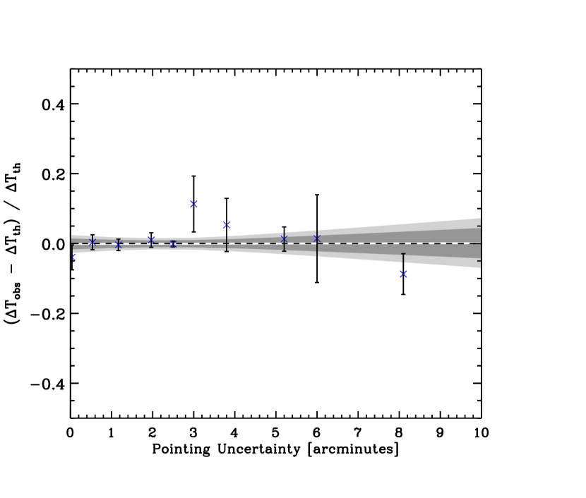
Figure 11: CMB data residuals plotted against pointing uncertainty. Six experiments do not quote pointing uncertainties so are omitted from this analysis. With the 6 experiments omitted, there are 170 degrees of freedom. The $\chi^{2}$ for the zero-line is 172.5 and the probability of finding a line that provides a better fit to the data is 57%. The $\chi^{2}$ for best-fitting line to the residual data is $172.5$ with a $\chi^{2}$ per degree of freedom of 1.01 for 170 degrees of freedom. The probability of finding a line that better fits the data is 57% so the best-fit line does not improve the fit beyond that of the zero-line. Thus, there is no evidence for a trend in this regression plot. Although, limiting the analysis to the 5 points with the largest uncertainties would indicate a trend, suggesting that the largest uncertainties may have been underestimated.

Testing for consistency with other CMB observations is another important way to identify possible systematic errors. When the areas of the sky observed overlap, this can be done by comparing CMB temperature maps (e.g. Ganga et al., 1994a; Lineweaver et al., 1995; Xu et al., 2001). When similar angular scales are being observed one can compare power spectra (e.g. Sievers et al., 2002, Figure 11). A prerequisite for the extraction of useful estimates for cosmological parameters from the combined CMB data set is the mutual consistency of the observational data points (Wang et al., 2002a); the best-fit must also be a good fit. Wang et al. (2002a) and Sievers et al. (2002) have recently explored the consistency of various CMB observations with respect to power spectrum models and concluded that the CMB fluctuation data is consistent with several minor exceptions.

Although individual observational groups vigorously test their data sets for systematic errors, the entire CMB observational data set has not yet been collectively tested. Here we check for consistency of the concordance model (Table 1) with respect to possible sources of systematic error. Under the assumption that the concordance model is the correct model (i.e. more correct than the best-fit to the CMB data alone), we explore residuals of the observational data with respect to this model to see if any patterns emerge. We attempt to identify systematic errors in the data that may have been ignored or only partially corrected for.

With only a few independent band power measurements the usefulness of such a strategy is compromised by low number statistics. However, we now have 203 measurements of band power on scales of $2<\ell<2000$ from over two dozen autonomous and semi-autonomous groups. There are enough CMB fluctuation detections from independent observations that subtle systematic effects could appear above the noise in regression plots of the data residuals. This is particularly the case when one has a better idea of the underlying model than provided by the CMB data alone.

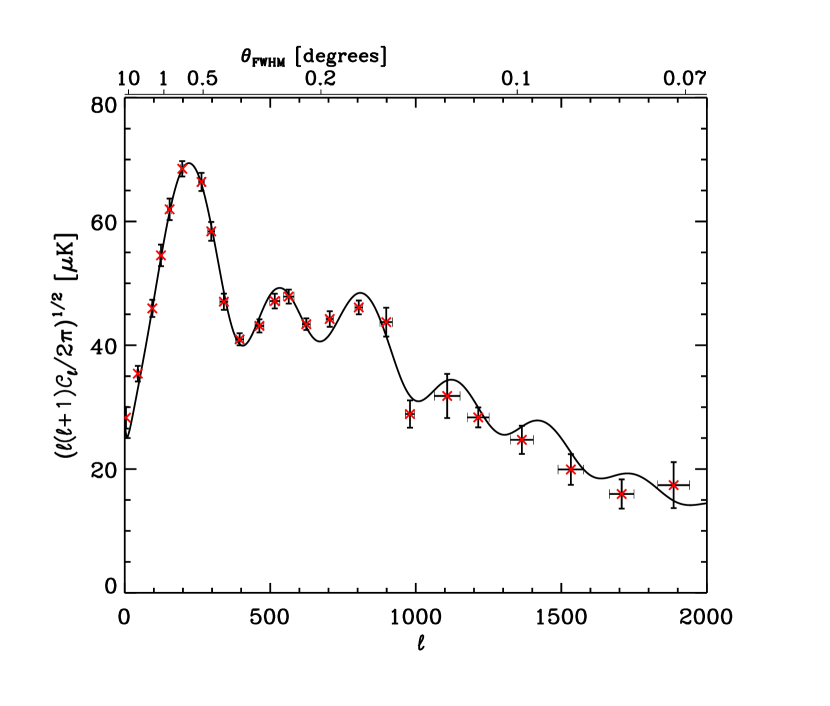
Figure 2: The concordance cosmology (Table 1) normalised to the full CMB data set is plotted with the binned observational data. The binning methodology is given in Appendix B. All statistical analyses detailed in this paper are performed on the raw, unbinned data given in Table B.

The history of the estimates of the position of the CMB dipole illustrates the idea. Once a relatively precise direction of the dipole was established, the positional scatter elongated in the direction of the galactic centre could be distinguished unambiguously from statistical scatter and more reliable corrections for galactic contamination could be made (Lineweaver, 1997, Figure 2). We aim to ascertain whether the use of the concordance model as a prior can help to separate statistical and systematic errors in the CMB anisotropy data. In §2 we discuss constraints on cosmological parameters, the current concordance model and how simultaneously analysing combinations of independent observational data sets can tighten cosmological constraints. Our analytical methodology is detailed in §3. In §4 possible sources of systematic uncertainty are discussed. In §5 and §6 our results are discussed and summarised.

2 THE CONCORDANCE COSMOLOGY

2.1 Observational concordance

The CMB has the potential to simultaneously constrain a number of cosmological parameters that are the ingredients of the hot big bang model. Unfortunately, particular parameter combinations can produce indistinguishable $C_{\ell}$ spectra (Efstathiou & Bond, 1999). For example, cosmological models with different matter content but the same geometry can have nearly identical anisotropies. Such model degeneracies limit parameter extraction from the CMB alone.

A number of recent analyses combine information from a range of independent observational data sets (e.g. Efstathiou et al., 2002; Lewis & Bridle, 2002; Sievers et al., 2002; Wang et al., 2002a, b), enabling certain degeneracies of the individual data sets to be resolved. As the observational data become more precise and diverse they form an increasingly tight network of parameter constraints. Analyses of a variety of astrophysical observations are beginning to refine an observationally concordant cosmological model.

Efstathiou et al. (2002) perform a combined likelihood analysis of the power spectra of the 2-degree Field Galaxy Redshift Survey (2dFGRS) and the CMB anisotropies under the assumptions that the galaxy power spectrum on large scales is directly proportional to the linear matter power spectrum and that the initial fluctuations were adiabatic, Gaussian and well described by power-laws with scalar and tensor indeces of $n_{s}$ and $n_{t}$. 11 cosmological parameter combinations are simultaneously considered; the curvature parameter $\Omega_{\kappa}$, the contribution to the overall energy density from the cosmological constant $\Omega_{\Lambda}$, $\omega_{b}=\Omega_{b}h^{2}$ (where $\Omega_{b}$ is the baryon energy density and $h$ the Hubble parameter), $\omega_{c}=\Omega_{c}h^{2}$ (where $\Omega_{c}$ is the energy density of CDM), the amplitude of scalar perturbations $A_{s}$, the ratio of tensor to scalar perturbations $A_{t}/A_{s}$, the spectral index of scalar perturbations $n_{s}$, that of tensor perturbations $n_{t}$, the reionisation optical depth $\tau$, the shape parameter that defines the turn-over of the matter power spectrum $\Gamma\simeq\Omega_{m}h$ (where $\Omega_{m}$ is the energy density of non-relativistic matter) and the bias parameter $b$. The big bang nucleosynthesis (BBN) constraint on the baryon content (Burles et al., 2001) is added to the analysis as a prior. The results for the CMB alone and combined analyses are given in Table 1.

Wang et al. (2002a) perform a similar analysis using the CMB data, the decorrelated linear power spectrum extracted from the PSC$z$ survey (Hamilton & Tegmark, 2002) and the Hubble Key Project (HKP) prior for $h$ (Freedman et al., 2001). Instead of assuming that the dark matter contribution to the energy density is entirely composed of cold dark matter, they explore the parameter combination $\omega_{d}=\Omega_{d}h^{2}$ and introduce a new parameter, $f_{\nu}=\Omega_{\nu}/\Omega_{d}$, that is the fraction of dark matter that is hot. Their constraints from the CMB alone and combined analyses are also given in Table 1.

Another recent analysis of the CMB data set is that of Sievers et al. (2002). They perform a likelihood analysis over 7 cosmological parameters ($\Omega_{\rm total}=1-\Omega_{\kappa}$, $\Omega_{\Lambda}$, $\omega_{b}$, $\omega_{c}$, $A_{s}$, $n_{s}$, $\tau$) applying a sequence of increasingly strong prior probabilities successively to the likelihood functions. These are a flat prior $\Omega_{\kappa}=0$ in accordance with the predictions of the simplest inflationary scenarios, a large scale structure prior that involves a constraint on the amplitude $\sigma_{8}^{2}$ and shape of the matter power spectrum, the HKP prior for $h$ and the $\Omega_{m}-\Omega_{\Lambda}$ priors from supernova type Ia (SNIa) observations (Riess et al., 1998; Perlmutter et al., 1999). Their results for the CMB alone and the CMB+priors likelihood analyses are also given in Table 1.

Lewis & Bridle (2002) implement a Markov chain Monte Carlo method to constrain 9 parameter flat models using a subsample of the CMB data set together with the BBN, HKP and SNIa priors. They also perform a combined analysis with the 2dFGRS. The most recent joint analysis of the CMB data set and the 2dFGRS is that of Wang et al. (2002b). The results of both these analysis are also given in Table 1.

Due to the degeneracies in the anisotropy power spectrum, the CMB alone is only able to provide weak constraints on particular cosmological parameters. Combining the CMB constraints with the results of independent observational data sets can tighten these constraints. The results of the joint likelihood analyses discussed in this section suggest the observationally concordant cosmology; $\Omega_{\kappa}\simeq 0$, $\Omega_{\Lambda}\simeq 0.7$ ($\Omega_{m}=\Omega_{b}+\Omega_{c}\simeq 0.3$), $\Omega_{b}h^{2}\simeq 0.02$, $n_{s}\simeq 1$ and $h\simeq 0.68$ with $A_{t}$, $\tau$ and $\Omega_{\nu}$ taken to be zero. With more precise and diverse cosmological observations, the ability of the standard $\Lambda$CDM cosmology to describe the observational universe will be extended and tested for inconsistencies.

2.2 Goodness of fit of the concordance cosmology to the CMB

We perform a simple $\chi^{2}$ calculation (see Appendix A) to determine the goodness-of-fit of this new standard $\Lambda$CDM cosmology to the CMB, employing the band power temperature measurements in Table B and their associated window functions. We limit our analysis to $2<\ell<2000$ because secondary anisotropy contributions, such as the Sunyaev-Zel’dovich (Sunyaev & Zel’dovich, 1970) effect, may dominate at $\ell>2000$ (e.g. Bond et al., 2002). The model radiation angular power spectrum is calculated using cmbfast (Seljak & Zaldarriaga, 1996). However, rather than adopting the cmbfast COBE-DMR normalisation, we implement the numerical approximation to marginalisation (see Appendix A) to find the optimal normalisation of the theoretical model to the full observational data set. We also similarly treat the beam uncertainties of BOOMERanG98 and MAXIMA1 as given by Lesgourgues & Liddle (2001) and the calibration uncertainties associated with the observations, treating them as free parameters with Gaussian distributions about their nominal values (see Eq. A7).

The minimised $\chi^{2}$ for the concordance model is 174.2. In order to determine how good a fit this model is to the observational data we need to know the number of degrees of freedom of the analysis. Although 203 degrees of freedom are provided by the number of observational data points (assuming they are uncorrelated), these are reduced by the number of concordance parameters that are constrained using the CMB data alone. The flatness of the concordance model ($\Omega_{\kappa}\simeq 0$) and the scale invariance of the primordial power spectrum of scalar perturbations ($n_{s}\simeq 1$) are extracted almost entirely from the CMB data. The remaining concordant parameters are more strongly constrained by non-CMB observations. We therefore estimate that 2 degrees of freedom should be subtracted from the original 203.

Within our analysis we marginalise over a number of nuisance parameters. We fit for 23 individual calibration constants, 2 beam uncertainties (those of BOOMERanG-98 and MAXIMA-1) and an overall normalisation. Thus a further 26 degrees of freedom must be subtracted leaving 175 degrees of freedom. The $\chi^{2}$ per degree of freedom is then 1.0, indicating that the concordance cosmology provides a good fit to the CMB data alone.

Data correlations other than the correlated beam and calibration uncertainties of individual experiments, that we take to have no inter-experiment dependence, are not considered in our analysis. Including such correlations would further reduce the number of degrees of freedom, increasing the $\chi^{2}$ per degree of freedom. However, our result is in agreement with the joint likelihood analyses that find that the cosmological model that best fits the CMB data is a better fit at the 1 or 2 $\sigma$ level than fit to the concordance model (Wang et al., 2002a).

We find the normalisation of the concordance model to the full CMB data set to be $Q_{10}=16.3\pm 0.1\,\mu$K, where $Q_{10}$ is defined through the relation (Linewaver & Barbosa, 1998),

$$10(10+1)C_{10}=\frac{24\pi}{5}\frac{Q_{10}^{2}}{T_{CMB}^{2}}\,.$$ (1)

The normalised concordance model is plotted with the calibrated and beam corrected observational data in Figure 1. It is difficult to distinguish the most important measurements because there are so many CMB data points on the plot and it is dominated by those with the largest error bars. Therefore, for clarity, we bin the data as described in Appendix B. The binned observations are plotted with the concordance cosmology in Figure 2. The linear $x$-axis emphasises the detail at small angular scales, clarifying measurements of the acoustic peaks.

3 EXAMINING THE RESIDUALS

Our analysis is based on the assumption that the combined cosmological observations used to determine the concordance model are giving us a more accurate estimate of cosmological parameters, and therefore of the true $C_{\ell}$ spectrum, than is given by the CMB data alone. Under this assumption, the residuals of the individual observed CMB band powers and the concordance $\Lambda$CDM model become tools to identify a variety of systematic errors. To this end, we create residuals, $R_{i}$, of the observed band power temperature anisotropies $\delta T_{i}^{\rm obs}\pm\sigma^{\rm obs}_{i}$ with respect to the concordant band powers $\delta T_{i}^{\rm th}$ such that,

$$R_{i}=\frac{\delta T_{i}^{\rm obs}-\delta T_{i}^{\rm th}}{\delta T_{i}^{\rm th}}\pm\frac{\sigma^{\rm obs}_{i}}{\delta T_{i}^{\rm th}}\,.$$ (2)

Systematic errors are part of the CMB band power estimates at some level. We examine our data residuals as functions of the instrument type, receivers, scan strategy and attitude control. Possible sources of systematic uncertainty are discussed in the following section and the instrumental and observational details that may be associated with systematic errors are listed in Table B. We look for any linear trends that may identify systematic effects that are correlated with these details of the experimental design. We quote the $\chi^{2}$ per degree of freedom of the best fitting line and the significance of the fit for each regression in Table 4. If the analysis determines that a linear trend can produce a significantly improved fit in comparison to that of a zero gradient line (zero-line) through the data, it may be indicative of an unidentified systematic source of uncertainty.

The zero-line through all the residual data gives a $\chi^{2}$ of 174.2. The analysis that determines the goodness-of-fit of the concordance model to the CMB data has 175 degrees of freedom. If the gradient and intercept were independent of the parameters varied to produce the concordance fit, the degrees of freedom would be further reduced by 2. However, the intercept of any line that fits the residual data will depend on the normalisation of the concordance model. We therefore subtract only one further degree of freedom, giving 174 degrees of freedom.

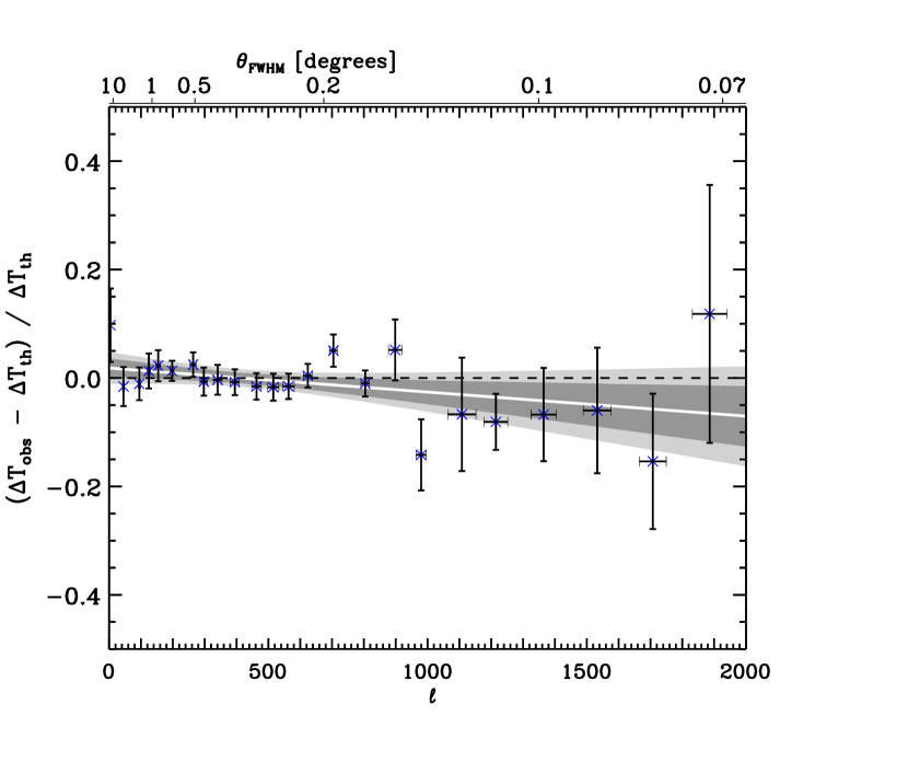
Figure 3: CMB data residuals plotted against $\ell$ (bottom $x$-axis) and angular scale (top $x$-axis). The fitting routine uses the $\ell$-range as an uncertainty in the $\ell$ value. The $\chi^{2}$ for the fit of the line to the data is 170.6 with a $\chi^{2}$ per degree of freedom of 0.98 for the 174 degrees of freedom. The probability of finding a line that better fits the data is 44% so the best-fit line is a better fit to the data than the zero-line. The zero-line is slightly outside the border of the 68% confidence region for the best-fit line so there is evidence for a trend in this regression plot at slightly greater than the 1-$\sigma$ level.

The best fitting zero-line fit to all the residual data has a $\chi^{2}$ per degree of freedom of 1.0 ($=174.2/174$). In order to determine the significance of a better fit provided by a linear trend, an understanding of the statistical effects of introducing the 2 parameters to the line-fitting analysis is required. For a 2-dimensional Gaussian distribution, the difference between the $\chi^{2}$ of the best-fit model and a model within the 68% confidence region of the best-fit model is less than 2.3 and for a model that is within the 95% confidence region of the best-fit model, this difference is less than 6.17 (Press et al., 1992). Our 68% and 95% contours in Figures 3 to 20 are so defined. The further the horizontal concordance zero-line is from the best fitting slope, the stronger the indication of a possible systematic error.

4 POSSIBLE SOURCES OF SYSTEMATIC UNCERTAINTY

4.1 Foregrounds

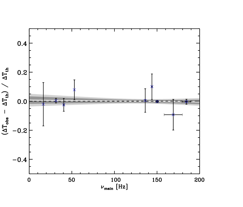
Figure 6: CMB data residuals plotted against the main frequency of individual instruments $\nu_{\rm main}$. The $\chi^{2}$ for the fit of the line to the data is $173.9$ with a $\chi^{2}$ per degree of freedom of 1.00 for the 174 degrees of freedom. The probability of finding a line that better fits the data is 51% so the best-fit line improves the fit beyond that of the zero-line only very slightly. Thus, there is no evidence for a trend in this regression plot.

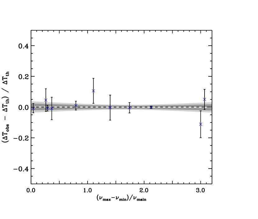
Figure 7: CMB data residuals plotted against the lever-arm in frequency $(\nu_{\rm max}-\nu_{\rm min})/\nu_{\rm main}$. The $\chi^{2}$ for the fit of the line to the data is $174.2$ with a $\chi^{2}$ per degree of freedom of 1.00 for the 174 degrees of freedom. The probability of finding a line that better fits the data is 52% so the best-fit line does not improve the fit beyond that of the zero-line. Thus, there is no evidence for a trend in this regression plot.

If foreground emission is present, it will raise the observed power. Galactic and extra-galactic signals from synchrotron, bremsstrahlung and dust emission have frequency dependencies that are different from that of the CMB (e.g. Tegmark & Efstathiou, 1996). If such contamination is present in the data, it may be revealed by a frequency dependence of the residuals (Figure 6). Multiple frequency observations provide various frequency lever-arms that allow individual groups to identify and correct for frequency dependent contamination. Experiments with broad frequency coverage may be better able to remove this contamination than those with narrow frequency coverage. We therefore examine the residuals as a function of the frequency lever-arm $(\nu_{\rm max}-\nu_{\rm min})/\nu_{\rm main}$ (Figure 7).

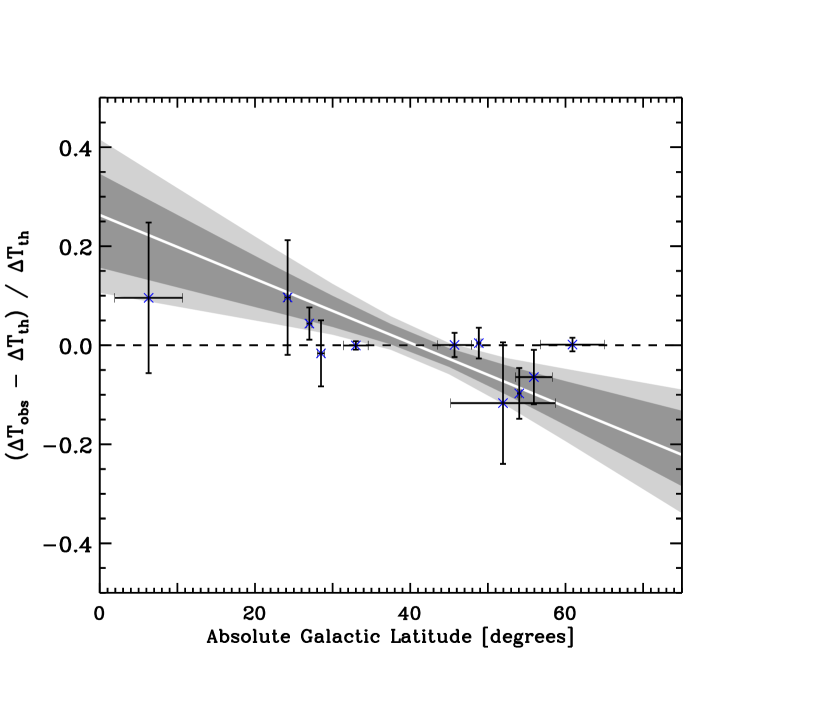
Figure 4: CMB data residuals plotted against absolute galactic latitude $|b|$. The fitting routine assumes that the uncertainty in $|b|$ extends to the limits of the $|b|$ range. The $\chi^{2}$ for the fit of the line to the data is 153.7 with a $\chi^{2}$ per degree of freedom of 0.88 for the 174 degrees of freedom. The probability of finding a line that better fits the data is 14% so the best-fit line is a much better fit to the data than the zero-line. The zero-line is outside the 95% confidence region for the best-fit line so there is a more than 2$\sigma$ trend in this regression plot that may be indicative of a systematic error associated with absolute galactic latitude.

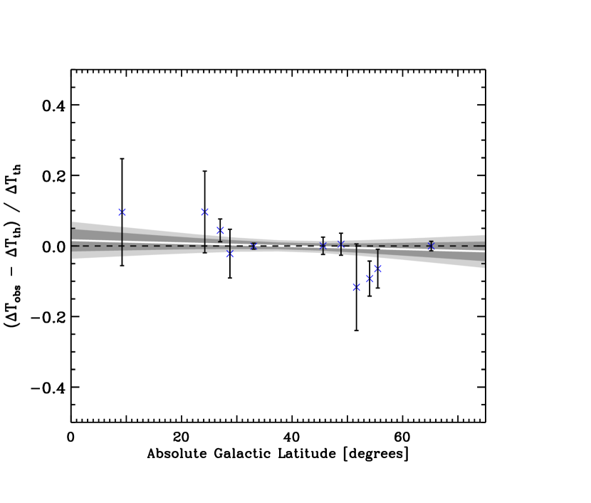
Figure 5: CMB data residuals plotted against the central absolute galactic latitude (i.e. the $x$-coordinate freedom has been removed from the fit). The $\chi^{2}$ for the fit of the line to the data is 173.5 with a $\chi^{2}$ per degree of freedom of 1.00 for the 174 degrees of freedom. The probability of finding a line that better fits the data is 50% so the best-fit line improves the fit beyond that of the zero-line only very slightly. Thus, we can conclude that there is no evidence for a trend in this regression plot.

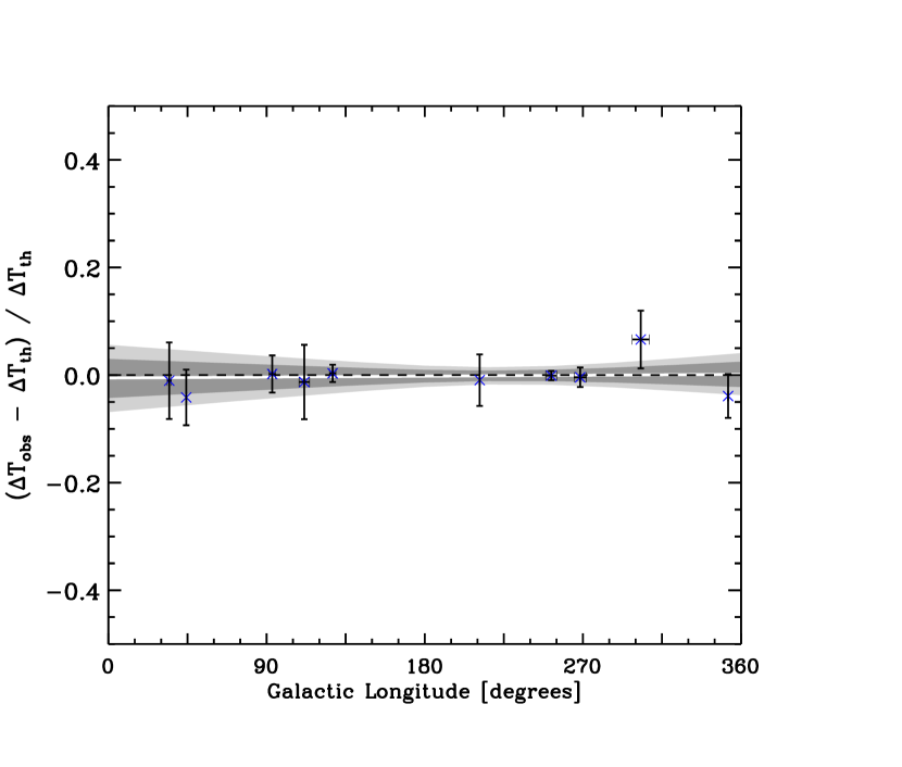
Figure 16: CMB data residuals plotted against galactic longitude. The VSA results quoted in the literature are the combined detections from 3 separate fields observed at various galactic longitudes. Information is not given in the literature to enable the contributions from the different fields to be separated, so the VSA experiment is omitted from this analysis. With the VSA experiment omitted, there are 159 degrees of freedom, the $\chi^{2}$ for the zero-line is 162.5 and the probability of finding a line that provides a better fit to the data is 59%. The $\chi^{2}$ for the fit of the line to the data is $162.4$ with a $\chi^{2}$ per degree of freedom of 0.98 for the 159 degrees of freedom. The probability of finding a line that better fits the data is 59% so the best-fit line does not improve the fit beyond that of the zero-line. Thus, there is no evidence for a trend in this regression plot.

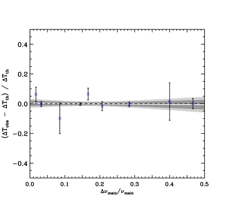
Figure 17: CMB data residuals plotted against bandwidth $\Delta\nu_{\rm main}/\nu_{\rm main}$. The $\chi^{2}$ for the fit of the line to the data is $174.1$ with a $\chi^{2}$ per degree of freedom of 1.00 for the 174 degrees of freedom. The probability of finding a line that better fits the data is 52% so the best-fit line does not improve the fit beyond that of the zero-line. Thus, there is no evidence for a trend in this regression plot.

Observations taken at lower absolute galactic latitudes, $|b|$, will be more prone to galactic contamination. In Figures 4, 16 and 5 we check for this effect by examining the residuals as a function of $|b|$ (Figures 4 and 5) and galactic longitude (Figure 16). Less likely would be a signal associated with the narrowness of the band pass of the main frequency channel $\Delta\nu_{\rm main}/\nu_{\rm main}$ (Figure 17).

4.2 Angular Scale-dependent effects

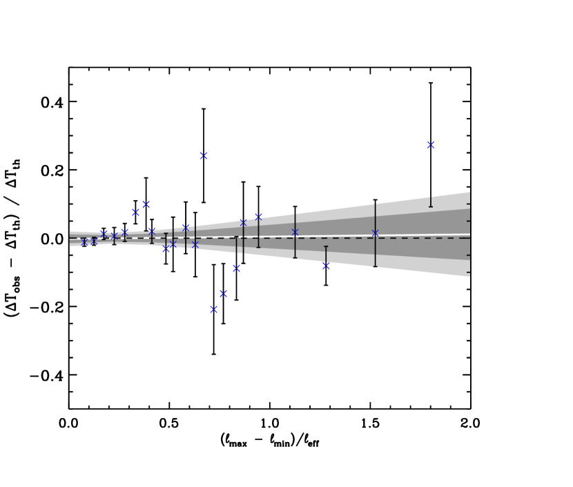
Figure 15: CMB data residuals plotted against width of $\ell$-space filter function $\Delta\ell/\ell$. The $\chi^{2}$ for the fit of the line to the data is $174.1$ with a $\chi^{2}$ per degree of freedom of 1.00 for the 174 degrees of freedom. The probability of finding a line that better fits the data is 52% so the best-fit line does not improve the fit beyond that of the zero-line. Thus, there is no evidence for a trend in this regression plot.

We examine scale-dependent uncertainties by plotting the residuals as a function of $\ell$ (Figure 3). The shape of the window function is most critical when the curvature of the power spectrum is large (at the extrema of the acoustic oscillations). We therefore explore the residuals as a function of the narrowness of the filter functions in $\ell$ space $\Delta\ell/\ell$ (Figure 15).

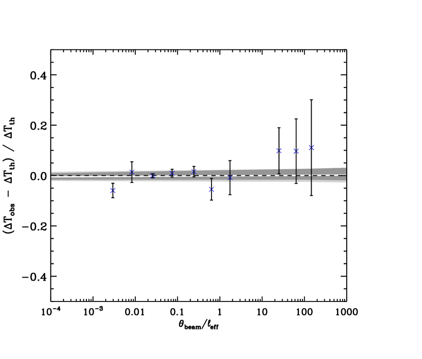
Figure 10: CMB data residuals plotted against $\theta_{beam}/\ell_{eff}$. The $x$-axis is logarithmic so as to best display the data and the residuals are examined for a linear trend with respect to the logarithmic resolution axis. The $\chi^{2}$ for the fit of the line to the data is $173.5$ with a $\chi^{2}$ per degree of freedom of 1.00 for the 174 degrees of freedom. The probability of finding a line that better fits the data is 50% so the best-fit line improves the fit beyond that of the zero-line only very slightly. Thus, there is no evidence for a trend in this regression plot.

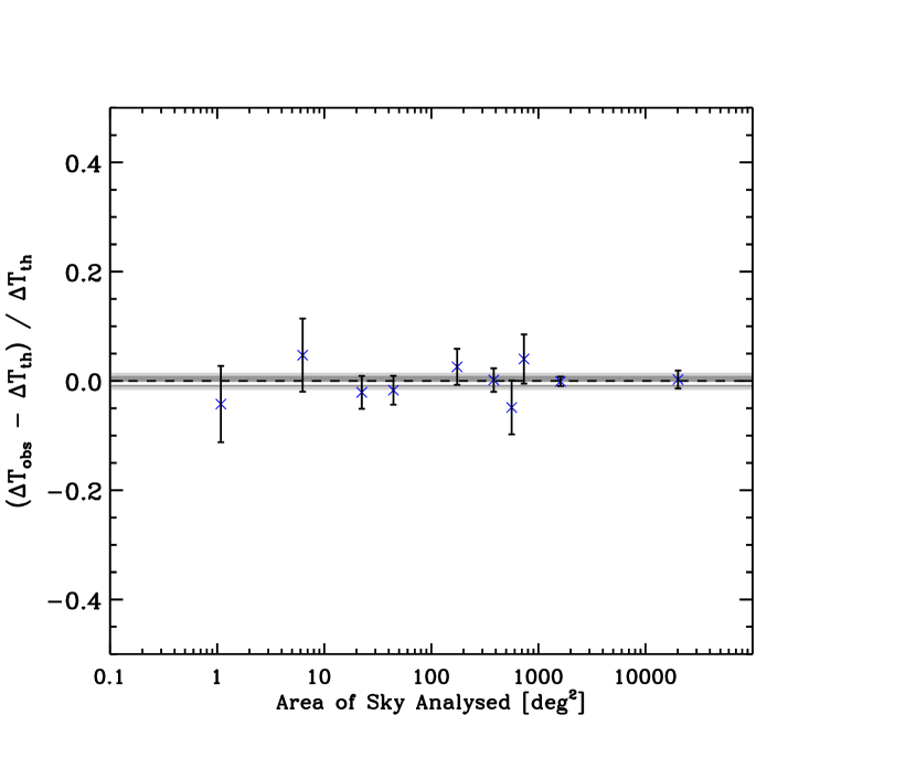
Figure 12: CMB data residuals plotted against area of sky. The area of sky axis is logarithmic so as to best display the data and the residuals are examined for a linear trend with respect to the logarithmic $x$-axis. The $\chi^{2}$ for the fit of the line to the data is $172.7$ with a $\chi^{2}$ per degree of freedom of 0.99 for the 174 degrees of freedom. The probability of finding a line that better fits the data is 49% so the best-fit line is a slightly better fit to the data than the zero-line. The zero-line is within the 68% confidence region for the best-fit line so there is no evidence for a significant trend in this regression plot.

The area of the sky observed determines the lowest $\ell$ probed while the beam size $\theta_{\rm beam}$ determines the highest $\ell$. The resolution of the instrument and the pointing uncertainty become increasingly important as fluctuations are measured at smaller angular scales. Small beams may be subject to unidentified smearing effects that may show up as a trend in the residual data with respect to $\theta_{beam}/\ell_{eff}$. Thus we examine the residuals as a function of the area of sky probed (Figure 12), $\theta_{beam}/\ell_{eff}$ (Figure 10) and pointing uncertainty (Figure 11) to look for hints of systematic errors associated with these factors.

4.3 Calibration

To analyse various experiments, knowledge of the calibration uncertainty of the measurements is necessary. Independent observations that calibrate off the same source will have calibration uncertainties that are correlated at some level and therefore a fraction of their freedom to shift upwards or downwards will be shared. For example, ACME-MAX, BOOMERanG97, CBI, MSAM, OVRO, TOCO and CBI all calibrate off Jupiter, so part of the quoted calibration uncertainties from these experiments will come from the brightness uncertainty of this source. The remainder will be due to detector noise and sample variance and should not have any such inter-experiment correlations. Wang et al. (2002a) perform a joint analysis of the CMB data making the approximation that the entire contribution to the calibration uncertainty from Jupiter’s brightness uncertainty is shared by the experiments that use this calibration source. The true correlation will be lower since the independent experiments observed Jupiter at different frequencies.

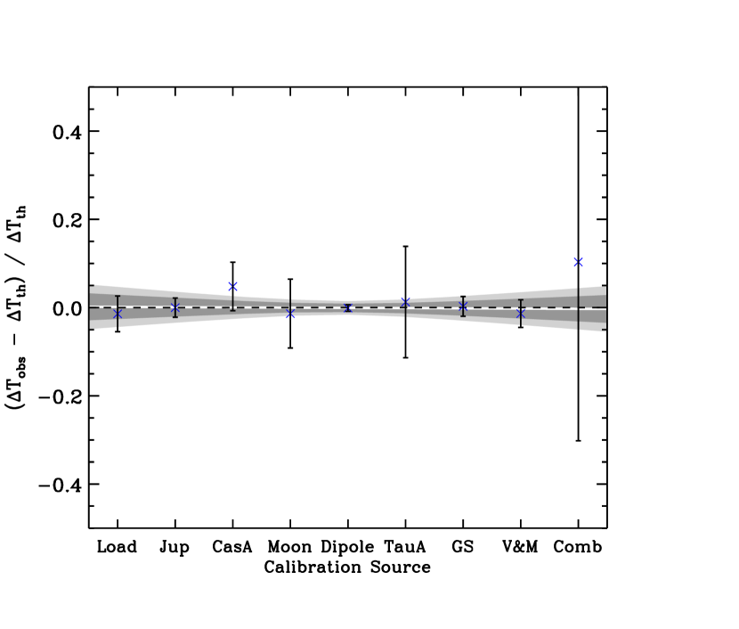
Figure 8: CMB data residuals plotted against calibration source. The $\chi^{2}$ for the fit of this line to the data is $174.2$ with a $\chi^{2}$ per degree of freedom of 1.00 for 174 degrees of freedom. The probability of finding a line that better fits the data is 52% so the best-fit line does not improve the fit beyond that of the zero-line. Thus, there is no evidence for a trend in this regression plot.

Inter-experiment correlations are not considered in our analysis, since we are unable to separate out the fraction of uncertainty that is shared by experiments. Instead we test for any calibration dependent systematics by examining the data residuals with respect to the calibration source (Figure 8). We note that including correlations between data points would reduce the number of degrees of freedom of our $\chi^{2}$ analysis.

4.4 Instrument type, platform and altitude

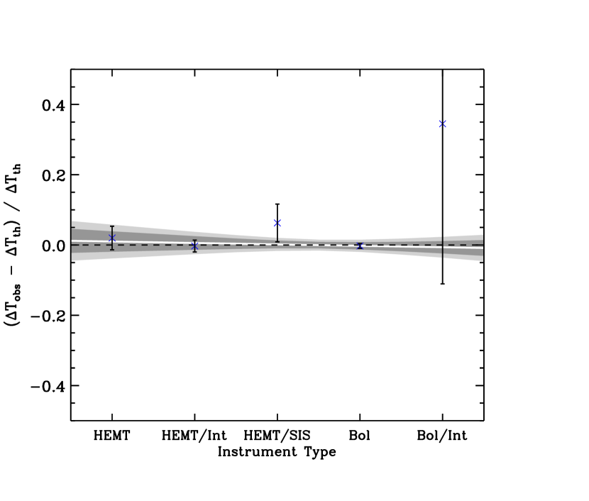
Figure 9: CMB data residuals plotted against instrument type. The $\chi^{2}$ for the fit of the line to the data is $173.9$ with a $\chi^{2}$ per degree of freedom of 1.00 for the 174 degrees of freedom. The probability of finding a line that better fits the data is 51% so the best-fit line improves the fit beyond that of the zero-line only very slightly. Thus, there is no evidence for a trend in this regression plot.

The experiments use combinations of 3 types of detector that operate over different frequency ranges. We classify the data with respect to their instrument type; HEMT interferometers (HEMT/Int), HEMT amplifier based non-interferometric instruments (HEMT), HEMT based amplifier and SIS based mixer combination instruments (HEMT/SIS), bolometric instruments and bolometric interferometers (Bol/Int). We check for receiver specific systematic effects by plotting the residuals as a function of instrument type (Figure 9).

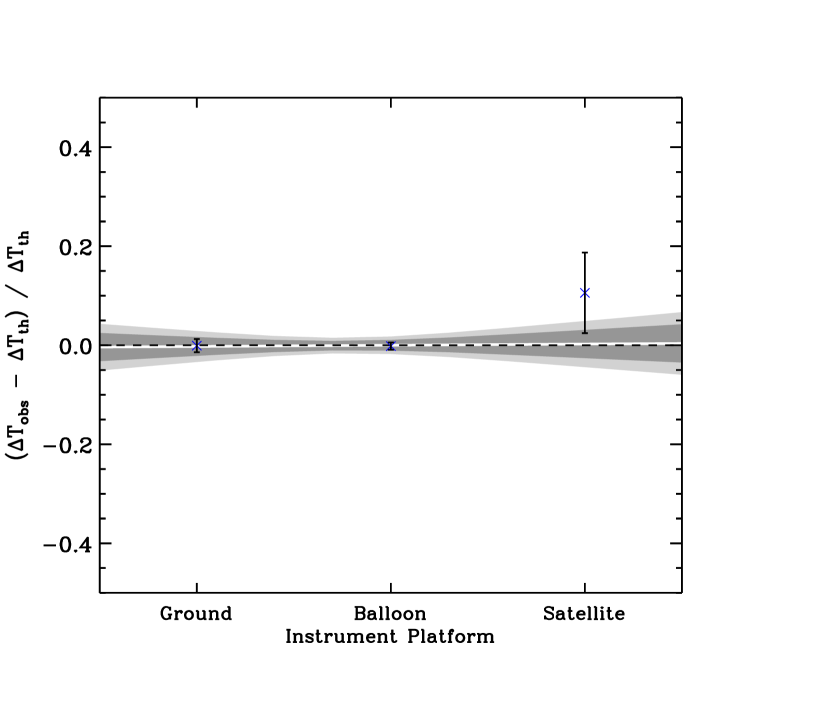
Figure 13: CMB data residuals plotted against instrument platform. The $\chi^{2}$ for the fit of the line to the data is $174.2$ with a $\chi^{2}$ per degree of freedom of 1.00 for the 174 degrees of freedom. The probability of finding a line that better fits the data is 52% so the best-fit line does not improve the fit beyond that of the zero-line. Thus, there is no evidence for a trend in this regression plot.

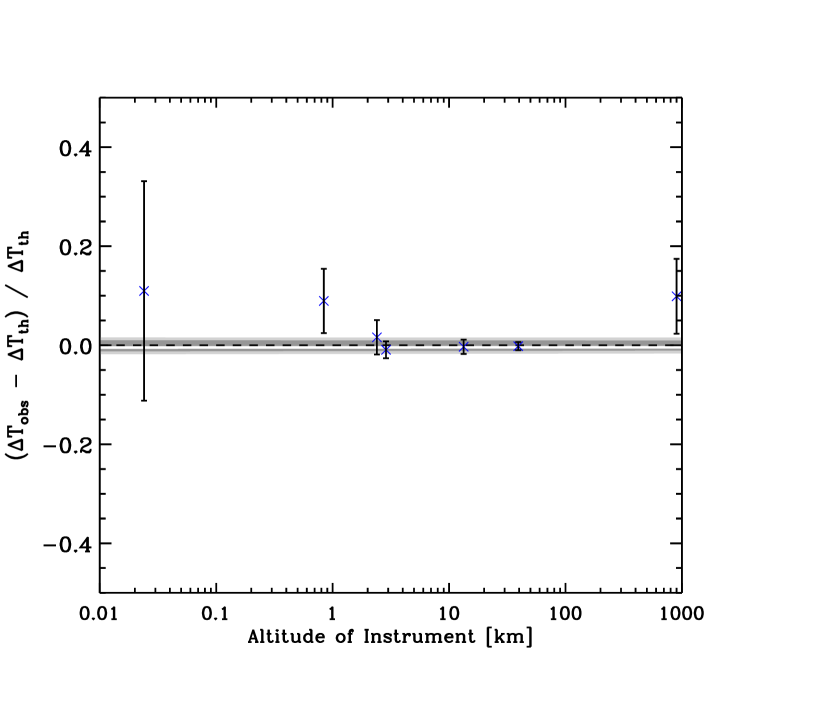
Figure 14: CMB data residuals plotted against instrument altitude. The $\chi^{2}$ for the fit of the line to the data is $172.6$ with a $\chi^{2}$ per degree of freedom of 0.99 for the 174 degrees of freedom. The probability of finding a line that better fits the data is 48% so the best-fit line is a slightly better fit to the data than the zero-line. The zero-line is within the 68% confidence region for the best-fit line so there is no evidence for a significant trend in this regression plot.

Water vapour in the atmosphere is a large source of contamination for ground based instruments. There may also be systematic errors associated with the temperature and stability of the thermal environment. We therefore explore instrument altitude (Figure 14) and platform (Figure 13) dependencies of the data residuals.

4.5 Random controls

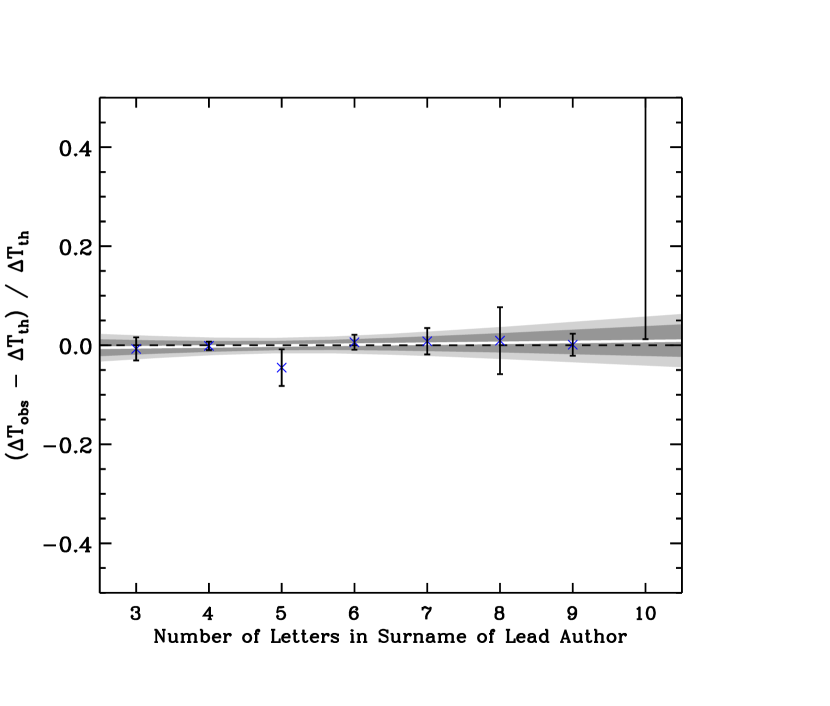
Figure 18: CMB data residuals plotted against the number of letters in the surname of the lead author of the published band-power estimates given in Table B. The $\chi^{2}$ for the fit of the line to the data is $174.0$ with a $\chi^{2}$ per degree of freedom of 1.00 for the 174 degrees of freedom. The probability of finding a line that better fits the data is 51% so the best-fit line improves the fit beyond that of the zero-line only very slightly. Therefore, as expected, there is no evidence of a significant trend in this plot.

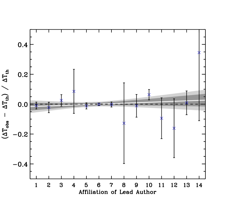
Figure 19: CMB data residuals plotted against the affiliation of the lead author of the published band-power estimates given in Table B (1:Berkeley, 2:CalTech, 3:Cambridge, 4:Carnegie Mellon, 5:Chicago, 6:Cleveland, 7:France, 8:Manchester, 9:Massachusetts, 10:Princeton, 11:Rome, 12:Santa Barbara, 13:Spain, 14:UBC). The $\chi^{2}$ for the fit of the line to the data is $173.2$ with a $\chi^{2}$ per degree of freedom of 1.00 for the 174 degrees of freedom. The probability of finding a line that better fits the data is 50% so the best-fit line improves the fit beyond that of the zero-line only very slightly. Therefore, as expected, there is no evidence of a significant trend in this plot.

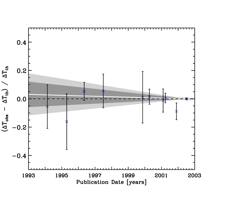
Figure 20: CMB data residuals plotted against the publication date of the band-power estimates given in Table B. The $\chi^{2}$ for the fit of the line to the data is $173.9$ with a $\chi^{2}$ per degree of freedom of 1.00 for the 174 degrees of freedom. The probability of finding a line that better fits the data is 51% so the best-fit line improves the fit beyond that of the zero-line only very slightly. Therefore, as expected, there is no evidence of a significant trend in this plot.

We use a number of control regressions to check that our analysis is working as expected. To this end, the residuals are examined with respect to the publication date of the band power data (Figure 20), the number of letters in the first author’s surname (Figure 18) and the affiliation of the last author (Figure 19). We expect the line fitted to these control regressions to be consistent with a zero-line through the residual data. Any significant improvement provided by a linear fit to these residuals may be indicative of a problem in the software or methodology.

5 RESULTS

For the regressions plotted, the residual data is binned as described in Appendix B so that any trends can be more effectively visualised. Since the data binning process may wash out any discrepancies between experiments, the linear fit analyses are performed on the unbinned data residuals. In Figures 3 to 20, the line that best-fits the data is plotted (solid white) and the 68% (dark grey) and 95% (light grey) confidence regions of the best-fit line are shaded. For each plot, we report the $\chi^{2}$ and the $\chi^{2}$ per degree of freedom for the best-fit line, the probability of finding a model that better fits the data and comment on the significance of the deviation of the zero-line (dashed black).

Our results are listed in Table 4 and imply that the most significant linear trend observable in the residuals is with respect to the absolute galactic latitude $|b|$ of the observations (see Figure 4). This trend is not eliminated by the removal of any one experiment and may be indicative of a source of galactic emission that has not been appropriately treated. The weighted average of points $|b|>40^{\circ}$ is $\sim-1\%$, while it is $\sim+1\%$ for $|b|<40^{\circ}$. If this is due to galactic contamination, then the normalisation Q₁₀ may have to be reduced to 16.1 $\mu$K.

For this regression, the errors in both the $y$ and $x$ direction are used in the fit. We have defined $|b|$ to be that of the centre of the observations and the uncertainties to extend to edges of the range. This allows the observations some freedom of the $x$-coordinate in the line-fitting analysis and may over-weight those detections that span small ranges in absolute galactic latitude. It is therefore also interesting to examine the residuals with respect to the central $|b|$ to determine the significance of the trend with the $x$-coordinate freedom removed (see Figure 5). The most plausible galactic latitude regression will be somewhere between the two plots.

Removing the $x$-coordinate freedom removes the significance of the trend. This result implies that experiments that observe over small ranges in galactic latitude are dominating the trend and we therefore can not simply correct for the systematic that is implied in (Figure 4). The comparison of rms levels in galactic dust (Finkbeiner et al., 1999) and synchrotron maps over the areas of CMB observations may help to clarify the interpretation of the trend. Such a technique has recently been applied to the MAXIMA1 data (Jaffe et al., 2003) but has yet to be performed on the full CMB data set.

Other plots also show some evidence for systematic errors. Figures 2 and 3 indicate that the 6 bins between $1000\leq\ell\leq 2000$ prefer a lower normalisation. This could be due to underestimates of beam sizes or pointing uncertainties or unidentified beam smearing effects at high $\ell$ for small beams. However, Figures 10 and 11 show no evidence for any trends, although limiting the pointing uncertainty analysis to the 5 points with the largest uncertainties would indicate a trend, suggesting that the largest pointing uncertainties may have been underestimated.

6 SUMMARY

Although individual observational groups vigorously test their data sets for systematic errors, the entire CMB observational data set has not yet been collectively tested. Under the assumption that the concordance model is the correct model, we have explored residuals of the observational data with respect to this model to see if any patterns emerge that may indicate a source of systematic error.

We have performed linear fits on the residual data with respect to many aspects of the observational techniques and, for the majority, we have found little or no evidence for any trends. However, there is significant evidence for an effect associated with $|b|$ that is not eliminated with the exclusion of any one data set. The data prefers a linear trend that is inconsistent at more than 95% confidence with a zero gradient line through the residuals. The best-fit line to the data suggests that CMB observations made closer to the galactic plane may be over-estimated by approximately 2%. A more detailed analysis of galactic dust and synchrotron maps may clarify the source of the indicated systematic uncertainty.

Appendix A $\chi^{2}$ MINIMISATION METHODOLOGY

For the observational power spectrum data quoted in the literature (Table B), individual $C_{\ell\,}$s are not estimated, rather band powers are given that average the power spectrum through a filter, or window function. Each theoretical model must therefore be re-expressed in the same form before a statistical comparison can be made.

The theoretical model can be re-expressed as $\delta T_{\ell_{\rm eff}}^{\rm th}$, using the method of Lineweaver et al. (1997). Boltzmann codes such as cmbfast (Seljak & Zaldarriaga, 1996) output theoretical power spectra in the form,

$$d_{1}({\ell})=\frac{\ell(\ell\,+\,1)}{2\pi}\,C_{\ell}^{\rm theory}\times{\rm normalisation}\,.$$ (A1)

Since the $C_{\ell}\,$s are adimensional, they are multiplied by $\bar{T}_{\rm CMB}^{2}\simeq(2.725\,{\rm K})^{2}$ (Mather et al., 1999) to express them in Kelvin,

$$d_{2}({\ell})\,=\,\bar{T}_{\rm CMB}^{2}\,d_{1}({\ell})\,.$$ (A2)

The sensitivity of each observation (denoted $i$) to a particular $\ell$ is incorporated using the observational window function $W_{\ell}$,

$$d_{3}(i,\,\ell)\,=\,d_{2}({\ell})\times\frac{(2\,\ell\,+1\,)\,W_{\ell}^{i}}{2\,\,\ell\,(\ell\,+\,1)}\,.$$ (A3)

The contribution from the model to the $i^{\rm th}$ observational band-power is determined and the influence of the window function removed,

$$D^{\rm th}_{i}\,=\,\frac{\sum_{\ell=2}^{\ell_{\rm max}}d_{3}(i,\,\ell)}{I(i)}\,,$$ (A4)

where $I$($i$) is the logarithmic integral of the window function,

$$I(i)\,=\sum_{\ell=2}^{\ell_{\rm max}}\frac{(2\,\ell\,+1\,)\,W_{\ell}^{i}}{2\,\,\ell\,(\ell\,+\,1)}\,.$$ (A5)

$\delta T_{\ell_{\rm eff}}^{\rm th}(i)$ is then,

$$\delta T_{\ell_{\rm eff}}^{\rm th}(i)=\sqrt{D^{\rm th}_{i}}\,,$$ (A6)

which can be statistically compared with the $i^{\rm th}$ observational band-power measurement $\delta T_{\ell_{\rm eff}}^{\rm obs}(i)\equiv\sqrt{D^{\rm obs}_{i}}$ given in Table B.

The assumption that the CMB signal is a Gaussian random variable enables analysis via a likelihood procedure. Due to the non-Gaussian distribution of the uncertainty in the band-power measurements, an accurate calculation of the likelihood function $L$ is non-trivial. However, approximations to the true likelihood have been derived (Bond et al., 2000; Bartlett et al., 2000). For example, the Bond et al. (2000) offset lognormal formalism is implemented in the publicly available radpack package. Unfortunately, the information necessary to implement this formalism has not yet been published by all observational groups. Therefore, in order to statistically analyse the complete CMB observational data set, we make the assumption that $L$ is Gaussian in $D_{i}$. Then,

$$\chi^{2}\equiv-2\ln{L}=\sum_{i}{\left(\frac{D^{\rm th}_{i}-D^{\rm obs}_{i}}{\sigma^{\rm obs}_{i}}\right)^{2}}.$$ (A7)

The normalisation of the primordial power spectrum is not predicted by inflationary scenarios and therefore the normalisation of the concordance model to the full CMB observational data set is a free parameter. Unless we are particularly interested in the amplitude of primordial fluctuations, we can treat the model normalisation $A$ as a nuisance parameter. Assuming a Gaussian likelihood, marginalisation can be approximated numerically for the power spectrum normalisation by computing the $\chi^{2}$ statistic of the concordance model for a number of discrete steps over the normalisation range. The normalisation that minimises the $\chi^{2}$ can thereby be determined for a particular theoretical model.

The CMB measurements have associated calibration uncertainties that allow data from the same instrument that is calibrated using the same source to shift collectively upwards or downwards. The calibration uncertainties $\sigma_{c}$ are given in Table B. The observational band-powers are multiplied by a calibration factor $C$ that can be treated as a nuisance parameter with a Gaussian distribution about 1. This introduces an additional $\chi^{2}$ term to Eq. A7 for each experiment that has an associated calibration uncertainty (see Eq. A8).

Additionally, the BOOMERanG98 and MAXIMA1 data sets have quantified beam and pointing uncertainties. The combined beam plus pointing uncertainty for each experiment introduces an additional term to Eq. A7 that is a function of $B$. $B$ can be treated as a nuisance parameter, with a Gaussian distribution in $B\sigma_{b,\,i}$ about 0 (see Eq. A8). Lesgourgues & Liddle (2001) give fitting functions for the combined beam plus pointing uncertainty in $D^{\rm obs}_{i}$ for each of these experiments; $\sigma_{b,\,\ell}=0.43\times 10^{-6}\ell^{2}$ for BOOMERanG98 and $\sigma_{b,\,\ell}=10^{-6}\ell^{1.7}$ for MAXIMA1.

The nuisance parameters are incorporated into Eq. A7 to give,

$$\chi^{2}=\sum_{i}{\left(\frac{A\,D^{\rm th}_{i}-\left(C_{k}+B_{k}\sigma_{b,\,i}\right)D^{\rm obs}_{i}}{\sigma_{i}}\right)^{2}}+\sum_{k}\left(\frac{C_{k}-1}{\sigma_{c,\,k}}\right)^{2}+\sum_{k}\left(B_{k}\right)^{2}\,,$$ (A8)

where the sum on $k$ is over the number of independent observational data sets. The numerical marginalisation approximation that takes discrete steps over nuisance parameters to find those that minimise the $\chi^{2}$ statistic is a computationally intensive technique. Each nuisance parameter introduced to the analysis increases the number of iterations of the $\chi^{2}$ minimisation process by a factor of the number of discrete steps taken over the nuisance parameter range. The assumption that the uncertainties in $D^{\rm obs}$ are Gaussian distributed enables an analytical approximation to be made that is computationally less time-consuming. However, since we are only interested in one cosmological model, the concordance $\Lambda$CDM model, we do not implement an analytical approximation here.

Appendix B OBSERVATIONAL DATA BINNING

The ever increasing number of CMB anisotropies has made data plots such as Figure 1 difficult to interpret. The solution is to compress the data in some way. Many of the more recent analyses have chosen to concentrate on the data from just one or two experiments, often the most recently released. However, this not only neglects potentially useful information, but can also unwittingly give more weight to particular observations that may suffer from associated systematic effects. We therefore choose to analyse all the available data.

One way to compress the data is to average them together into single band-power bins in $\ell$-space. Such an approach has been taken by a number of authors (e.g. Knox & Page, 2000; Jaffe et al., 2001; Wang et al., 2002a). Providing that the uncertainty in the data is Gaussian and correlations between detections are treated appropriately, narrow band power bins can be chosen that will retain all cosmological information.

Band-power measurements from independent observations that overlap in the sky will be correlated to some extent. Such correlations can only be treated by jointly analysing the combined overlapping maps to extract band power estimates that are uncorrelated or have explicitly defined correlation matrices. This process of data compression will wash out any systematics associated with a particular data set, so data consistency checks are vital before this stage. If the map data is unavailable, the crude assumption that independent observations are uncorrelated in space must be made. This assumption is made in likelihood analyses performed on the full power spectrum data set and, since inclusion of these correlations would reduce the degrees of freedom of an analysis, the goodness-of-fit of a particular model to the data is better than it should be.

Some observational groups publish matrices encoding the correlations of their individual band-power measurements. To some extent, the calibration uncertainties of experiments that calibrate using the same source are also correlated. Bond et al. (2000) describe a data binning technique that takes a lognormal noise distribution that is approximately Gaussian and incorporates the correlation weight matrices of individual experiments. Wang et al. (2002a) detail a method to treat partial correlations of calibration uncertainties. Both are useful to produce statistically meaningful data bins.

Data binning averages out any evidence for discrepancies between independent observations and, in practice, data uncertainties are rarely Gaussian and the information required to treat correlated data is not always available. So although data binning is useful for visualisation purposes, statistical analyses of the binned observations will generally give different results from those performed on the raw data.

The statistical analyses detailed in this paper are performed on the published CMB band power measurements given in Table B. Binned data plots are presented purely to aid the interpretation of results. Therefore each calibrated and, for BOOMERanG98 and MAXIMA1, beam corrected observational data point is binned assuming it to be entirely uncorrelated. Bin widths must be carefully chosen so that important features of the data are not smoothed out, especially in regions of extreme curvature. For example, in the case of the power spectrum, an unwisely chosen bin that spans an acoustic maximum will average out the power in the bin to produce a binned data point that misleadingly assigns less power to the peak.

The contribution from the $i$th observational measurement ($x_{i}\pm\sigma_{x,\,i}$, $y_{i}\pm\sigma_{y,\,i}$) to a binned point ($x_{b}\pm\sigma_{x,\,b}$, $y_{b}\pm\sigma_{y,\,b}$) is weighted by the square inverse of its variance,

$$x_{b}\,\pm\,\sigma_{x,\,b}\,=\,\frac{\sum_{i}x_{i}\,\sigma_{x,\,i}^{-2}}{\sum_{i}\sigma_{x,\,i}^{-2}}\,\pm\,\sqrt{\frac{1}{\sum_{i}\sigma_{x,\,i}^{-2}}}\,,$$ (B1)

$$y_{b}\,\pm\,\sigma_{y,\,b}\,=\,\frac{\sum_{i}y_{i}\,\sigma_{y,\,i}^{-2}}{\sum_{i}\sigma_{y,\,i}^{-2}}\,\pm\,\sqrt{\frac{1}{\sum_{i}\sigma_{y,\,i}^{-2}}}\,.$$ (B2)

If quoted error bars are uneven, a first guess for the binned data point is obtained by averaging the uncertainties. A more accurate estimate can then be converged upon by iterating over the binning routine, inserting the positive variance for measurements that are below the bin averaged point and negative variance for those that are above.

All the data from a particular experiment will be measured using the same instrument and therefore can be binned together for the purpose of visualising any trends in the data residuals with respect to the instrument design. When data from the same experiment is placed in the same bin, the variance of the resultant binned data point can be easily adjusted to account for any correlated calibration uncertainty associated with the observational data. A degree of freedom is reduced for each independent calibration uncertainty. This effectively tightens the constraints on the binned data.

For example, if $n$ calibrated data points in a bin have equal variance $\sigma_{y}$ and an entirely correlated calibration uncertainty, they share $n-1$ degrees of freedom and their contribution to the variance of the binned data point is then $\sigma_{y}/\sqrt{n-1}$. When each of the $n$ data points have different variances, their contribution to the uncertainty in the binned data point is given by,

$$\sigma_{y,\,b}\,=\,\frac{1}{\sqrt{\sum_{j}\sigma_{y,\,j}^{-2}-\left(n\,/\,\sum_{j}\sigma_{y,\,j}\right)^{2}}}\,.$$ (B3)

This method of binning is employed when appropriate to produce the plotted residual data bins.

Figure 1: The concordance cosmology (Table 1) normalised to the full CMB data set is plotted with the recalibrated and, for BOOMERanG98 and MAXIMA1, beam corrected CMB observational data given in Table B that spans the scales $2<\ell<2000$.

Table 1: 1-$\sigma$ cosmological parameter constraints from 5 independent analyses.

	Efstathiou et al. (2002)		Wang et al. (2002a)		Sievers et al. (2002)		Lewis & Bridle (2002)		Wang et al. (2002b)		$\Lambda$CDM concordance
	CMB alone	+2dFGRS+BBN	CMB alone	+PSC$z$+HKP	CMB alone	+priorsa	CMB+priorsb	+2dFGRS	CMB+flat prior	+2dFGRS
$\Omega_{k}$	$-0.04^{+.05}_{-.32}$	$-0.013^{+.027}_{-.019}$	$-0.05^{+.05}_{-.17}$	$0.02^{+.03}_{-.04}$	$-0.05\pm.05$	(0.00)	(0.00)	(0.00)	(0.00)	(0.00)	0.0
$\Omega_{\Lambda}$	$0.43^{+.23}$	$0.73\pm.04$	$0.57^{+.16}_{-.23}$	$0.65^{+.05}_{-.09}$	$0.54^{+.12}_{-.13}$	$0.70^{+.02}_{-.03}$	$0.72\pm 0.06$	$0.71\pm 0.04$	$0.71\pm 0.11$	$0.72\pm 0.09$	0.7
$\omega_{b}$	$0.020^{+.013}_{-.002}$	$0.020\pm.001$	$0.021^{+.005}_{-.003}$	$0.020^{+.005}_{-.002}$	$0.023\pm.003$	$0.024^{+.002}_{-.003}$	$0.022\pm.001$	$0.022\pm.001$	0.023$\pm$.003	0.024$\pm$.003	0.02
$\omega_{c}$	$0.13^{+.03}_{-.05}$	$0.10^{+.02}_{-.01}$	-	-	$0.13^{+.03}_{-.02}$	$0.12^{+.01}_{-.01}$	-	-	0.112$\pm$.014	0.115$\pm$.013	0.12
$\omega_{d}$	-	-	$0.10^{+.02}_{-.03}$	$0.12^{+.03}_{-.02}$	-	-	0.099$\pm$.014	0.106$\pm$.010	-	-	0.12
$f_{\nu}$	-	-	$0.08^{+0.30}$	$0.04^{+.08}$	-	-	$<0.10$	$<0.04$	-	-	0
$n_{s}$	$0.96^{+.27}_{-.04}$	$1.04^{+.06}_{-.05}$	$0.91^{+.08}_{-.05}$	$0.93^{+.06}_{-.05}$	$1.02^{+.06}_{-.07}$	$1.04^{+.05}_{-.06}$	1.02$\pm$.05	1.03$\pm$.05	0.99$\pm$.06	0.99$\pm$.04	1.0
$\tau$	$<0.25$	$<0.25$	$<0.09$	$<0.14$	$0.16^{+.18}_{-.13}$	$0.13^{+.13}_{-.10}$	-	-	$0.04^{+0.06}$	$0.06\pm.03$	0
$\Omega_{m}h$	-	$0.19\pm.02$	-	-	-	-	0.18$\pm$.03	0.19$\pm$.02	-	-	0.2
$h$	-	$0.66^{+.09}_{-.03}$	$0.42^{+.12}_{-.09}$	$0.71^{+.06}_{-.06}$	$0.55^{+.09}_{-.09}$	$0.69^{+.02}_{-.02}$	0.67$\pm$.05	0.66$\pm$.03	0.71$\pm$.13	0.73$\pm$.11	0.68

Table 2: The current compilation of CMB observational data from $\ell=2$ to $\ell=2000$.

Experiment	Ref.	$\ell_{{\rm eff}}$	$\ell_{{\rm min}}$	$\ell_{{\rm max}}$	$\delta T_{\ell_{\rm eff}}^{\rm obs}\pm\sigma^{\rm obs}$	$\sigma_{c}^{a}$	Publication Date
					$(\mu$K)	(%)	(yrs)
ACBAR	[1]	187.0	75.0	300.0	$82.3_{-8.5}^{+7.7}$	10.0	2002.9
ACBAR	[1]	389.0	307.0	459.0	$53.6_{-6.0}^{+5.4}$	10.0	2002.9
ACBAR	[1]	536.0	462.0	602.0	$52.1_{-5.0}^{+4.6}$	10.0	2002.9
ACBAR	[1]	678.0	615.0	744.0	$47.1_{-4.0}^{+3.7}$	10.0	2002.9
ACBAR	[1]	842.0	751.0	928.0	$48.0_{-3.9}^{+3.6}$	10.0	2002.9
ACBAR	[1]	986.0	921.0	1048.0	$28.2_{-2.9}^{+2.6}$	10.0	2002.9
ACBAR	[1]	1128.0	1040.0	1214.0	$36.1_{-3.0}^{+2.8}$	10.0	2002.9
ACBAR	[1]	1279.0	1207.0	1352.0	$24.1_{-2.9}^{+2.6}$	10.0	2002.9
ACBAR	[1]	1426.0	1338.0	1513.0	$25.1_{-2.8}^{+2.5}$	10.0	2002.9
ACBAR	[1]	1580.0	1510.0	1649.0	$18.7_{-3.2}^{+2.7}$	10.0	2002.9
ACBAR	[1]	1716.0	1648.0	1785.0	$15.7_{-3.5}^{+2.9}$	10.0	2002.9
ACBAR	[1]	1866.0	1782.0	1953.0	$19.0_{-3.9}^{+3.2}$	10.0	2002.9
ACME-MAX	[2]	139.0	72.0	247.0	$49.4_{-7.8}^{+7.8}$	-	1996.7
ACME-SP91	[3]	61.0	30.0	102.0	$30.3_{-8.9}^{+5.6}$	-	1995.3
ACME-SP94	[3]	61.0	30.0	102.0	$36.3_{-14.1}^{+6.9}$	-	1995.3
ARCHEOPS	[4]	18.5	15.0	22.0	$28.1_{-12.2}^{+8.3}$	7.0	2002.8
ARCHEOPS	[4]	28.5	22.0	35.0	$30.6_{-4.0}^{+3.6}$	7.0	2002.8
ARCHEOPS	[4]	40.0	35.0	45.0	$34.6_{-4.0}^{+3.6}$	7.0	2002.8
ARCHEOPS	[4]	52.5	45.0	60.0	$30.2_{-4.0}^{+3.5}$	7.0	2002.8
ARCHEOPS	[4]	70.0	60.0	80.0	$39.9_{-2.9}^{+2.7}$	7.0	2002.8
ARCHEOPS	[4]	87.5	80.0	95.0	$44.2_{-3.3}^{+3.1}$	7.0	2002.8
ARCHEOPS	[4]	102.5	95.0	110.0	$51.2_{-3.3}^{+3.1}$	7.0	2002.8
ARCHEOPS	[4]	117.5	110.0	125.0	$51.8_{-3.6}^{+3.4}$	7.0	2002.8
ARCHEOPS	[4]	135.0	125.0	145.0	$58.8_{-3.1}^{+3.0}$	7.0	2002.8
ARCHEOPS	[4]	155.0	145.0	165.0	$60.7_{-3.4}^{+3.2}$	7.0	2002.8
ARCHEOPS	[4]	175.0	165.0	185.0	$67.7_{-3.5}^{+3.3}$	7.0	2002.8
ARCHEOPS	[4]	197.5	185.0	210.0	$69.3_{-3.5}^{+3.3}$	7.0	2002.8
ARCHEOPS	[4]	225.0	210.0	240.0	$67.5_{-3.6}^{+3.4}$	7.0	2002.8
ARCHEOPS	[4]	257.5	240.0	275.0	$71.1_{-3.5}^{+3.4}$	7.0	2002.8
ARCHEOPS	[4]	292.5	275.0	310.0	$57.5_{-5.1}^{+4.7}$	7.0	2002.8
ARCHEOPS	[4]	330.0	310.0	350.0	$51.3_{-4.8}^{+4.4}$	7.0	2002.8
ARGO1	[5]	95.0	51.0	173.0	$39.1_{-8.7}^{+8.7}$	-	1994.1
ARGO2	[6]	95.0	51.0	173.0	$46.8_{-9.5}^{+12.1}$	-	1996.4
BAM	[7]	74.0	27.0	156.0	$55.6_{-31.6}^{+18.8}$	-	1997.2
BOOM97	[8]	58.0	25.0	75.0	$29.0_{-11.0}^{+13.0}$	8.0	2000.4
BOOM97	[8]	102.0	76.0	125.0	$49.0_{-9.0}^{+9.0}$	8.0	2000.4
BOOM97	[8]	153.0	126.0	175.0	$67.0_{-9.0}^{+10.0}$	8.0	2000.4
BOOM97	[8]	204.0	176.0	225.0	$72.0_{-10.0}^{+10.0}$	8.0	2000.4
BOOM97	[8]	255.0	226.0	275.0	$61.0_{-12.0}^{+11.0}$	8.0	2000.4
BOOM97	[8]	305.0	276.0	325.0	$55.0_{-15.0}^{+14.0}$	8.0	2000.4
BOOM97	[8]	403.0	326.0	475.0	$32.0_{-22.0}^{+13.0}$	8.0	2000.4
BOOM98	[9]	50.5	26.0	75.0	$37.7_{-4.4}^{+3.9}$	10.0	2002.9
BOOM98	[9]	100.5	76.0	125.0	$51.1_{-2.8}^{+2.7}$	10.0	2002.9
BOOM98	[9]	150.5	126.0	175.0	$69.4_{-2.8}^{+2.7}$	10.0	2002.9
BOOM98	[9]	200.5	176.0	225.0	$71.7_{-2.5}^{+2.4}$	10.0	2002.9
BOOM98	[9]	250.5	226.0	275.0	$73.2_{-2.2}^{+2.2}$	10.0	2002.9
BOOM98	[9]	300.5	276.0	325.0	$62.9_{-1.8}^{+1.7}$	10.0	2002.9
BOOM98	[9]	350.5	326.0	375.0	$49.4_{-1.4}^{+1.4}$	10.0	2002.9
BOOM98	[9]	400.5	376.0	425.0	$42.7_{-1.2}^{+1.2}$	10.0	2002.9
BOOM98	[9]	450.5	426.0	475.0	$45.7_{-1.3}^{+1.3}$	10.0	2002.9
BOOM98	[9]	500.5	476.0	525.0	$49.6_{-1.4}^{+1.3}$	10.0	2002.9
BOOM98	[9]	550.5	526.0	575.0	$49.4_{-1.4}^{+1.3}$	10.0	2002.9
BOOM98	[9]	600.5	576.0	625.0	$47.1_{-1.4}^{+1.4}$	10.0	2002.9
BOOM98	[9]	650.5	626.0	675.0	$44.7_{-1.5}^{+1.5}$	10.0	2002.9
BOOM98	[9]	700.5	676.0	725.0	$46.8_{-1.7}^{+1.6}$	10.0	2002.9
BOOM98	[9]	750.5	726.0	775.0	$44.8_{-2.0}^{+1.9}$	10.0	2002.9
BOOM98	[9]	800.5	776.0	825.0	$50.8_{-2.2}^{+2.1}$	10.0	2002.9
BOOM98	[9]	850.5	826.0	875.0	$47.2_{-2.7}^{+2.5}$	10.0	2002.9
BOOM98	[9]	900.5	876.0	925.0	$47.5_{-3.2}^{+3.0}$	10.0	2002.9
BOOM98	[9]	950.5	926.0	975.0	$34.0_{-5.3}^{+4.6}$	10.0	2002.9
BOOM98	[9]	1000.5	976.0	1025.0	$34.0_{-7.1}^{+5.8}$	10.0	2002.9
CAT1	[10]	397.0	322.0	481.0	$50.8_{-15.4}^{+15.4}$	10.0	1996.3
CAT1	[10]	615.0	543.0	717.0	$49.0_{-13.6}^{+19.1}$	10.0	1996.3
CAT2	[11]	397.0	322.0	481.0	$57.3_{-13.6}^{+10.9}$	10.0	1999.8
CAT2	[11]	615.0	543.0	717.0	$0.0_{-0.0}^{+54.6}$	10.0	1999.8
CBI-1a	[12]	603.0	437.0	783.0	$64.0_{-9.0}^{+11.0}$	5.0	2001.2
CBI-1a	[12]	1190.0	966.0	1451.0	$31.0_{-5.0}^{+7.0}$	5.0	2001.2
CBI-1b	[12]	603.0	437.0	783.0	$52.0_{-9.0}^{+11.0}$	5.0	2001.2
CBI-1b	[12]	1190.0	966.0	1451.0	$28.0_{-7.0}^{+10.0}$	5.0	2001.2
CBI-D8h	[13]	307.0	2.0	500.0	$80.8_{-31.5}^{+22.3}$	5.0	2002.4
CBI-D8h	[13]	640.0	500.0	880.0	$56.7_{-13.0}^{+10.5}$	5.0	2002.4
CBI-D8h	[13]	1133.0	880.0	1445.0	$32.3_{-6.7}^{+5.5}$	5.0	2002.4
CBI-D8h	[13]	1703.0	1445.0	2010.0	$21.2_{-7.7}^{+5.5}$	5.0	2002.4
CBI-D14h	[13]	307.0	2.0	500.0	$91.5_{-35.8}^{+25.3}$	5.0	2002.4
CBI-D14h	[13]	640.0	500.0	880.0	$30.2_{-30.2}^{+13.3}$	5.0	2002.4
CBI-D14h	[13]	1133.0	880.0	1445.0	$17.6_{-17.6}^{+10.2}$	5.0	2002.4
CBI-D14h	[13]	1703.0	1445.0	2010.0	$0.0_{-0.0}^{+10.0}$	5.0	2002.4
CBI-D20h	[13]	307.0	2.0	500.0	$82.6_{-25.3}^{+19.2}$	5.0	2002.4
CBI-D20h	[13]	640.0	500.0	880.0	$36.4_{-10.0}^{+7.8}$	5.0	2002.4
CBI-D20h	[13]	1133.0	880.0	1445.0	$26.0_{-5.7}^{+4.7}$	5.0	2002.4
CBI-D20h	[13]	1703.0	1445.0	2010.0	$24.0_{-6.1}^{+4.9}$	5.0	2002.4
CBI-M2h	[14]	304.0	0.0	400.0	$27.0_{-16.0}^{+9.0}$	5.0	2002.4
CBI-M2h	[14]	496.0	400.0	600.0	$48.0_{-8.0}^{+7.0}$	5.0	2002.4
CBI-M2h	[14]	696.0	600.0	800.0	$41.0_{-7.0}^{+6.0}$	5.0	2002.4
CBI-M2h	[14]	896.0	800.0	1000.0	$48.0_{-7.0}^{+6.0}$	5.0	2002.4
CBI-M2h	[14]	1100.0	1000.0	1200.0	$31.0_{-8.0}^{+6.0}$	5.0	2002.4
CBI-M2h	[14]	1300.0	1200.0	1400.0	$15.0_{-15.0}^{+10.0}$	5.0	2002.4
CBI-M2h	[14]	1502.0	1400.0	1600.0	$13.0_{-13.0}^{+12.0}$	5.0	2002.4
CBI-M2h	[14]	1702.0	1600.0	1800.0	$0.0_{-0.0}^{+22.0}$	5.0	2002.4
CBI-M2h	[14]	1899.0	1800.0	2000.0	$0.0_{-0.0}^{+17.0}$	5.0	2002.4
CBI-M14h	[14]	304.0	0.0	400.0	$65.0_{-15.0}^{+12.0}$	5.0	2002.4
CBI-M14h	[14]	496.0	400.0	600.0	$50.0_{-9.0}^{+7.0}$	5.0	2002.4
CBI-M14h	[14]	696.0	600.0	800.0	$51.0_{-7.0}^{+7.0}$	5.0	2002.4
CBI-M14h	[14]	896.0	800.0	1000.0	$41.0_{-7.0}^{+6.0}$	5.0	2002.4
CBI-M14h	[14]	1100.0	1000.0	1200.0	$27.0_{-8.0}^{+6.0}$	5.0	2002.4
CBI-M14h	[14]	1300.0	1200.0	1400.0	$30.0_{-8.0}^{+6.0}$	5.0	2002.4
CBI-M14h	[14]	1502.0	1400.0	1600.0	$34.0_{-9.0}^{+7.0}$	5.0	2002.4
CBI-M14h	[14]	1702.0	1600.0	1800.0	$0.0_{-0.0}^{+16.0}$	5.0	2002.4
CBI-M20h	[14]	304.0	0.0	400.0	$60.0_{-16.0}^{+13.0}$	5.0	2002.4
CBI-M20h	[14]	496.0	400.0	600.0	$49.0_{-5.0}^{+5.0}$	5.0	2002.4
CBI-M20h	[14]	696.0	600.0	800.0	$36.0_{-8.0}^{+6.0}$	5.0	2002.4
CBI-M20h	[14]	896.0	800.0	1000.0	$42.0_{-8.0}^{+7.0}$	5.0	2002.4
CBI-M20h	[14]	1100.0	1000.0	1200.0	$43.0_{-8.0}^{+7.0}$	5.0	2002.4
CBI-M20h	[14]	1300.0	1200.0	1400.0	$30.0_{-13.0}^{+9.0}$	5.0	2002.4
CBI-M20h	[14]	1502.0	1400.0	1600.0	$37.0_{-13.0}^{+9.0}$	5.0	2002.4
CBI-M20h	[14]	1702.0	1600.0	1800.0	$27.0_{-27.0}^{+11.0}$	5.0	2002.4
CBI-M20h	[14]	1899.0	1800.0	2000.0	$11.0_{-11.0}^{+18.0}$	5.0	2002.4
COBE-DMR	[15]	2.1	2.0	2.5	$8.5_{-8.5}^{+16.0}$	0.7	1996.0
COBE-DMR	[15]	3.1	2.5	3.7	$28.0_{-10.3}^{+7.5}$	0.7	1996.0
COBE-DMR	[15]	4.1	3.4	4.8	$34.0_{-7.2}^{+6.0}$	0.7	1996.0
COBE-DMR	[15]	5.6	4.7	6.6	$25.1_{-6.6}^{+5.3}$	0.7	1996.0
COBE-DMR	[15]	8.0	6.8	9.3	$29.4_{-4.1}^{+3.6}$	0.7	1996.0
COBE-DMR	[15]	10.9	9.7	12.2	$27.7_{-4.5}^{+3.9}$	0.7	1996.0
COBE-DMR	[15]	14.4	12.8	15.7	$26.1_{-5.2}^{+4.4}$	0.7	1996.0
COBE-DMR	[15]	19.4	16.6	22.1	$33.0_{-5.4}^{+4.6}$	0.7	1996.0
DASI	[16]	118.0	104.0	167.0	$61.4_{-7.1}^{+6.3}$	4.0	2002.2
DASI	[16]	203.0	173.0	255.0	$72.7_{-3.9}^{+3.7}$	4.0	2002.2
DASI	[16]	289.0	261.0	342.0	$60.5_{-2.9}^{+2.7}$	4.0	2002.2
DASI	[16]	377.0	342.0	418.0	$40.6_{-2.5}^{+2.4}$	4.0	2002.2
DASI	[16]	465.0	418.0	500.0	$43.5_{-2.6}^{+2.5}$	4.0	2002.2
DASI	[16]	553.0	506.0	594.0	$53.3_{-2.8}^{+2.7}$	4.0	2002.2
DASI	[16]	641.0	600.0	676.0	$40.9_{-3.4}^{+3.2}$	4.0	2002.2
DASI	[16]	725.0	676.0	757.0	$44.8_{-4.1}^{+3.7}$	4.0	2002.2
DASI	[16]	837.0	763.0	864.0	$48.2_{-4.9}^{+4.5}$	4.0	2002.2
FIRS	[17]	11.0	2.0	28.0	$29.4_{-7.8}^{+7.7}$	-	1994.7
IAB	[18]	120.0	65.0	221.0	$94.5_{-41.8}^{+41.8}$	-	1993.6
IACB94	[19]	33.0	17.0	59.0	$111.9_{-60.1}^{+65.4}$	14.0	1998.3
IACB94	[19]	53.0	34.0	79.0	$54.6_{-21.9}^{+27.2}$	14.0	1998.3
IACB96	[20]	39.0	15.0	77.0	$34.0_{-6.0}^{+8.0}$	10.0	2001.1
IACB96	[20]	61.0	39.0	89.0	$40.0_{-6.0}^{+7.0}$	10.0	2001.1
IACB96	[20]	81.0	61.0	108.0	$41.0_{-8.0}^{+8.0}$	10.0	2001.1
IACB96	[20]	99.0	81.0	123.0	$50.0_{-9.0}^{+10.0}$	10.0	2001.1
IACB96	[20]	116.0	102.0	139.0	$46.0_{-9.0}^{+10.0}$	10.0	2001.1
IACB96	[20]	134.0	122.0	154.0	$56.0_{-10.0}^{+11.0}$	10.0	2001.1
JBIAC	[21]	109.0	90.0	128.0	$43.0_{-13.3}^{+12.3}$	-	1999.8
MAXIMA1	[22]	77.0	36.0	110.0	$44.7_{-6.1}^{+7.0}$	4.0	2001.3
MAXIMA1	[22]	147.0	111.0	185.0	$54.4_{-5.4}^{+5.9}$	4.0	2001.3
MAXIMA1	[22]	222.0	186.0	260.0	$78.1_{-6.0}^{+6.5}$	4.0	2001.3
MAXIMA1	[22]	294.0	261.0	335.0	$61.9_{-4.9}^{+5.2}$	4.0	2001.3
MAXIMA1	[22]	381.0	336.0	410.0	$47.6_{-5.2}^{+5.6}$	4.0	2001.3
MAXIMA1	[22]	449.0	411.0	485.0	$38.3_{-4.5}^{+4.8}$	4.0	2001.3
MAXIMA1	[22]	523.0	486.0	560.0	$44.0_{-4.9}^{+5.1}$	4.0	2001.3
MAXIMA1	[22]	597.0	561.0	635.0	$42.6_{-5.5}^{+5.6}$	4.0	2001.3
MAXIMA1	[22]	671.0	636.0	710.0	$45.8_{-6.4}^{+6.4}$	4.0	2001.3
MAXIMA1	[22]	746.0	711.0	785.0	$46.8_{-7.9}^{+7.7}$	4.0	2001.3
MAXIMA1	[22]	856.0	786.0	935.0	$55.7_{-7.1}^{+6.8}$	4.0	2001.3
MAXIMA1	[22]	1004.0	936.0	1085.0	$32.9_{-32.9}^{+15.1}$	4.0	2001.3
MAXIMA1	[22]	1147.0	1086.0	1235.0	$14.9_{-14.9}^{+40.0}$	4.0	2001.3
MSAM	[23]	84.0	39.0	130.0	$35.0_{-11.0}^{+15.0}$	5.0	2000.2
MSAM	[23]	201.0	131.0	283.0	$49.0_{-8.0}^{+10.0}$	5.0	2000.2
MSAM	[23]	407.0	284.0	453.0	$47.0_{-6.0}^{+7.0}$	5.0	2000.2
OVRO	[24]	589.0	361.0	756.0	$59.0_{-8.6}^{+6.5}$	-	2000.2
PyI-III	[25]	87.0	49.0	105.0	$60.0_{-5.0}^{+9.0}$	20.0	1997.0
PyI-III	[25]	170.0	120.0	239.0	$66.0_{-9.0}^{+10.7}$	20.0	1997.0
PyV	[26]	50.0	21.0	94.0	$30.0_{-4.0}^{+4.0}$	15.0	2001.9
PyV	[26]	74.0	35.0	130.0	$29.0_{-5.0}^{+5.0}$	15.0	2001.9
PyV	[26]	108.0	67.0	157.0	$33.0_{-6.0}^{+6.0}$	15.0	2001.9
PyV	[26]	140.0	99.0	185.0	$35.0_{-10.0}^{+10.0}$	15.0	2001.9
PyV	[26]	172.0	132.0	215.0	$54.0_{-16.0}^{+15.0}$	15.0	2001.9
PyV	[26]	203.0	164.0	244.0	$90.0_{-23.0}^{+23.0}$	15.0	2001.9
PyV	[26]	233.0	195.0	273.0	$67.0_{-55.0}^{+33.0}$	15.0	2001.9
PyV	[26]	264.0	227.0	303.0	$0.0_{-0.0}^{+72.0}$	15.0	2001.9
QMAP	[27]	80.0	39.0	121.0	$48.3_{-7.5}^{+6.4}$	8.0	2002.4
QMAP	[27]	111.0	47.0	175.0	$54.6_{-5.3}^{+5.3}$	8.0	2002.4
QMAP	[27]	126.0	72.0	180.0	$60.9_{-7.5}^{+6.4}$	8.0	2002.4
SK	[27]	87.0	58.0	126.0	$50.2_{-5.2}^{+8.3}$	10.0	2002.4
SK	[27]	166.0	123.0	196.0	$70.5_{-6.2}^{+7.3}$	10.0	2002.4
SK	[27]	237.0	196.0	266.0	$86.8_{-8.3}^{+10.4}$	10.0	2002.4
SK	[27]	286.0	248.0	310.0	$87.9_{-10.4}^{+12.5}$	10.0	2002.4
SK	[27]	349.0	308.0	393.0	$70.4_{-29.1}^{+19.8}$	10.0	2002.4
Tenerife	[28]	20.0	12.0	30.0	$30.0_{-15.0}^{+11.0}$	-	2000.0
TOCO97	[27]	63.0	45.0	81.0	$35.1_{-6.4}^{+10.2}$	10.0	2002.4
TOCO97	[27]	86.0	64.0	102.0	$43.0_{-6.3}^{+6.9}$	10.0	2002.4
TOCO97	[27]	114.0	90.0	134.0	$67.3_{-5.8}^{+6.3}$	10.0	2002.4
TOCO97	[27]	158.0	135.0	180.0	$86.4_{-7.1}^{+7.2}$	10.0	2002.4
TOCO97	[27]	199.0	170.0	237.0	$82.9_{-7.6}^{+7.6}$	10.0	2002.4
TOCO98	[27]	128.0	95.0	154.0	$53.7_{-16.3}^{+18.1}$	8.0	2002.4
TOCO98	[27]	152.0	114.0	178.0	$80.6_{-10.8}^{+10.8}$	8.0	2002.4
TOCO98	[27]	226.0	170.0	263.0	$81.6_{-7.9}^{+6.9}$	8.0	2002.4
TOCO98	[27]	306.0	247.0	350.0	$68.8_{-10.8}^{+9.8}$	8.0	2002.4
TOCO98	[27]	409.0	344.0	451.0	$23.3_{-22.4}^{+22.4}$	8.0	2002.4
VIPER	[29]	108.0	30.0	228.0	$61.0_{-22.0}^{+31.0}$	8.0	2000.3
VIPER	[29]	173.0	73.0	288.0	$77.0_{-20.0}^{+26.0}$	8.0	2000.3
VIPER	[29]	237.0	126.0	336.0	$65.0_{-17.0}^{+24.0}$	8.0	2000.3
VIPER	[29]	263.0	150.0	448.0	$79.0_{-14.0}^{+18.0}$	8.0	2000.3
VIPER	[29]	422.0	291.0	604.0	$28.0_{-15.0}^{+15.0}$	8.0	2000.3
VIPER	[29]	589.0	448.0	796.0	$65.0_{-25.0}^{+25.0}$	8.0	2000.3
VSA	[30]	160.0	100.0	190.0	$62.2_{-10.0}^{+11.7}$	3.5	2002.9
VSA	[30]	220.0	190.0	250.0	$76.8_{-9.3}^{+10.0}$	3.5	2002.9
VSA	[30]	289.0	250.0	310.0	$73.4_{-7.8}^{+8.3}$	3.5	2002.9
VSA	[30]	349.0	310.0	370.0	$51.0_{-5.7}^{+5.5}$	3.5	2002.9
VSA	[30]	416.0	370.0	450.0	$41.8_{-4.4}^{+4.0}$	3.5	2002.9
VSA	[30]	479.0	450.0	500.0	$40.5_{-7.4}^{+7.3}$	3.5	2002.9
VSA	[30]	537.0	500.0	580.0	$53.5_{-5.4}^{+5.3}$	3.5	2002.9
VSA	[30]	605.0	580.0	640.0	$38.2_{-8.0}^{+7.7}$	3.5	2002.9
VSA	[30]	670.0	640.0	700.0	$47.3_{-6.8}^{+6.8}$	3.5	2002.9
VSA	[30]	726.0	700.0	750.0	$43.8_{-9.5}^{+8.3}$	3.5	2002.9
VSA	[30]	795.0	750.0	850.0	$59.9_{-5.6}^{+5.2}$	3.5	2002.9
VSA	[30]	888.0	850.0	950.0	$38.4_{-7.9}^{+7.6}$	3.5	2002.9
VSA	[30]	1002.0	950.0	1050.0	$0.0_{-0.0}^{+33.0}$	3.5	2002.9
VSA	[30]	1119.0	1050.0	1200.0	$33.5_{-11.6}^{+9.1}$	3.5	2002.9
VSA	[30]	1271.0	1200.0	1350.0	$0.0_{-0.0}^{+37.8}$	3.5	2002.9
VSA	[30]	1419.0	1350.0	1700.0	$36.2_{-31.5}^{+17.2}$	3.5	2002.9

References. — [1] Kuo et al. (2002), [2] Tanaka et al. (1996), Lineweaver (1998), [3] Benoît et al. (2002), [4] Gunderson et al. (1995), [5] de Bernardis et al. (1994), [6] Masi et al. (1996), [7] Tucker et al. (1997), [8] Mauskopf et al. (2000), [9] Ruhl et al. (2002), [10] Scott et al. (1996), [11] Baker et al. (1999), [12] Padin et al. (2001), [13] Mason et al. (2002), [14] Pearson et al. (2002), [15] Tegmark & Hamilton (1997), [16] Halverson et al. (2002), [17] Ganga et al. (1994a), [18] Piccirillo & Calisse (1993), [19] Femenia et al. (1998), [20] Romeo et al. (2001), [21] Dicker et al. (1999), [22] Lee et al. (2001), [23] Wilson et al. (2000), [24] Leitch et al. (2000), [25] Platt et al. (1997), [26] Coble et al. (2001), [27] Miller et al. (2002), [28] Gutierrez et al. (2000), [29] Peterson et al. (2000), [30] Grainge et al. (2002).

Table 3: Details of the CMB observational techniques.

Experiment	Ref.	$\nu_{\rm main}$	$\Delta\nu_{\rm main}$	$\nu$ Range	$\theta_{\rm beam}$ FWHM	Point. Uncert.a	Area of	Calibration	Instrument	Platform	Inst. Alt.	$|$Gal. Lat.$|$	Gal. Long.
		(GHz)	(GHz)	(GHz)	(arcmin)	(arcmin)	Sky (deg2)	Source	Type		(m)	Range (deg)	Range (deg)
ACBAR	[1]	150.0	15.0	150.0 - 280.0	4.5	0.30	24.8	Venus & Mars	Bolometer	Ground	2.9	36.7 - 57.0	250.3 - 276.5
ACME-MAX	[2]	180.0	7.0	105.0 - 420.0	30.0	1.00	18.8	Jupiter	Bolometer	Balloon	35.4	40.8 - 76.6	67.4 - 108.5
ACME-SP91	[3]	27.7	1.2	27.7 - 27.7	96.0	5.00	44.0	Taurus A	HEMT	Ground	2.8	45.0 - 55.0	275.0 - 305.0
ACME-SP94	[4]	35.0	1.2	27.7 - 41.5	83.0	7.20	20.0	H/C Load	HEMT	Ground	2.8	40.0 - 55.0	270.0 - 290.0
ARCHEOPS	[5]	190.0	31.0	143.0 - 545.0	8.0	1.50	5198.0	Dipole	Bolometer	Balloon	34.0	30.0 - 90.0	30.0 - 220.0
ARGO1	[6]	150.0	15.0	150.0 - 600.0	52.0	2.00	26.0	H/C Load	Bolometer	Balloon	40.0	22.0 - 35.0	64.0 - 79.0
ARGO2	[7]	150.0	15.0	150.0 - 600.0	52.0	2.00	10.0	H/C Load	Bolometer	Balloon	40.0	0.0 - 7.8	33.8 - 35.7
BAM	[8]	147.0	20.0	111.0 - 255.0	42.0	3.00	1.0	Jupiter	Bol/Int	Balloon	41.5	12.8 - 32.8	100.3 - 108.0
BOOM97	[9]	153.0	21.0	96.0 - 153.0	18.0	1.00	365.0	Jupiter	Bolometer	Balloon	38.5	11.0 - 83.0	17.0 - 178.0
BOOM98	[10]	150.0	11.0	90.0 - 410.0	11.1	2.50	1213.0	Dipole	Bolometer	Balloon	39.0	18.0 - 45.0	239.0 - 266.0
CAT1	[11]	16.5	0.2	13.5 - 16.5	117.6	-	4.0	Cas A	HEMT/Int	Ground	0.0	29.5 - 38.0	140.5 - 151.9
CAT2	[12]	16.5	0.2	13.5 - 16.5	117.6	-	4.0	Cas A	HEMT/Int	Ground	0.0	33.9 - 40.4	90.1 - 98.9
CBI-1a	[13]	31.0	0.5	26.5 - 35.5	3.0	0.03	1.1	Taurus A	HEMT/Int	Ground	5.1	23.3 - 25.0	229.7 - 230.9
CBI-1b	[13]	31.0	0.5	26.5 - 35.5	3.0	0.03	1.1	Taurus A	HEMT/Int	Ground	5.1	47.8 - 49.1	348.0 - 350.3
CBI-D8h	[14]	31.0	0.5	26.5 - 35.5	3.0	0.03	1.1	Jupiter	HEMT/Int	Ground	5.1	23.3 - 25.0	229.7 - 230.9
CBI-D14h	[14]	31.0	0.5	26.5 - 35.5	3.0	0.03	1.1	Jupiter	HEMT/Int	Ground	5.1	53.4 - 54.8	356.4 - 358.7
CBI-D20h	[14]	31.0	0.5	26.5 - 35.5	3.0	0.03	1.1	Jupiter	HEMT/Int	Ground	5.1	27.6 - 29.3	43.9 - 45.0
CBI-M2h	[15]	31.0	0.5	26.5 - 35.5	3.0	0.05	40.0	Jupiter	HEMT/Int	Ground	5.1	53.0 - 55.0	175.0 - 177.0
CBI-M14h	[15]	31.0	0.5	26.5 - 35.5	3.0	0.05	40.0	Jupiter	HEMT/Int	Ground	5.1	48.0 - 50.0	347.0 - 351.0
CBI-M20h	[15]	31.0	0.5	26.5 - 35.5	3.0	0.05	40.0	Jupiter	HEMT/Int	Ground	5.1	26.0 - 28.0	42.0 - 45.0
COBE-DMR	[16]	53.0	0.1	31.5 - 90.0	420.0	3.00	41253.0	H/C Load	HEMT	Satellite	900.0	20.0 - 90.0	0.0 - 360.0
DASI	[17]	31.0	0.5	26.5 - 35.5	20.0	2.00	400.0	Gal. Sources	HEMT/Int	Ground	2.8	26.9 - 67.3	254.7 - 324.4
FIRS	[18]	167.0	19.0	167.0 - 682.0	228.0	60.00	14000.0	Dipole	Bolometer	Balloon	36.3	0.0 - 80.0	45.0 - 200.0
IAB	[19]	136.0	1.5	136.0 - 136.0	50.0	2.00	6.0	H/C Load	Bolometer	Ground	3.3	22.2 - 32.1	297.4 - 308.4
IACB94	[20]	116.0	1.5	90.9 - 272.7	121.8	5.40	150.0	Moon	Bolometer	Ground	2.4	0.0 - 49.2	63.5 - 128.9
IACB96	[21]	142.9	1.5	96.8 - 272.7	81.0	5.40	1000.0	Moon	Bolometer	Ground	2.4	0.0 - 87.8	41.3 - 204.1
JBIAC	[22]	33.0	1.5	33.0 - 33.0	120.0	-	260.0	Moon	HEMT/Int	Ground	2.4	0.0 - 76.0	65.0 - 181.0
MAXIMA1	[23]	150.0	35.0	150.0 - 410.0	10.0	0.95	57.0	Dipole	Bolometer	Balloon	37.0	44.0 - 54.3	84.7 - 100.5
MSAM	[24]	170.0	22.5	170.0 - 680.0	30.0	2.50	10.0	Jupiter	Bolometer	Balloon	39.0	25.0 - 36.0	113.0 - 120.0
OVRO	[25]	31.7	3.0	14.5 - 31.7	7.4	2.00	6.0	Jupiter	HEMT	Ground	1.2	25.1 - 29.3	120.6 - 125.3
PyI-III	[26]	90.0	18.0	90.0 - 90.0	45.0	6.00	121.0	H/C Load	Bolometer	Ground	2.8	60.0 - 70.0	270.0 - 355.0
PyV	[27]	40.3	2.8	40.3 - 40.3	60.0	9.00	598.0	H/C Load	HEMT	Ground	2.8	30.0 - 70.0	270.0 - 355.0
QMAP	[28]	37.0	3.1	31.0 - 42.0	48.0	3.60	527.0	Cas A	HEMT	Balloon	30.0	8.0 - 46.0	102.0 - 132.0
SK	[29]	42.0	3.5	31.0 - 42.0	28.0	1.80	200.0	Cas A	HEMT	Ground	0.5	19.0 - 35.0	114.0 - 132.0
Tenerife	[30]	15.0	0.8	10.0 - 15.0	300.0	-	2000.0	Combination	HEMT	Ground	2.4	40.0 - 90.0	40.0 - 210.0
TOCO97	[31]	37.0	3.0	31.0 - 144.0	48.0	0.45	600.0	Jupiter	HEMT/SIS	Ground	5.2	0.0 - 55.0	270.0 - 335.0
TOCO98	[31]	144.0	1.7	31.0 - 144.0	12.0	0.45	600.0	Jupiter	HEMT/SIS	Ground	5.2	0.0 - 55.0	270.0 - 335.0
VIPER	[32]	40.0	3.0	40.0 - 40.0	15.6	4.00	4.0	H/C Load	HEMT	Ground	2.8	50.0 - 60.0	330.0 - 342.0
VSA	[33]	34.0	0.8	34.0 - 34.0	120.0	5.00	140.0	Jupiter	HEMT/Int	Ground	2.4	31.5 - 54.3	-b

References. — [1] Kuo et al. (2002), [2] Alsop et al. (1992), Lim et al. (1996), Tanaka et al. (1996), [3] Gunderson et al. (1995), [4] Benoît et al. (2002) [5] Ganga et al. (1994b), Gunderson et al. (1995), [6] de Bernardis et al. (1993), de Bernardis et al. (1994), [7] de Bernardis et al. (1993), de Bernardis et al. (1994), Masi et al. (1995), Masi et al. (1996), [8] Tucker et al. (1997), [9] Mauskopf et al. (2000), Piacentini et al. (2002), [10] Crill et al. (2002), Netterfield et al. (2002), Ruhl et al. (2002), [11] Scott et al. (1996), [12] Baker et al. (1999), [13] Padin et al. (2001), Padin et al. (2002), [14] Mason et al. (2002), [15] Mason et al. (2002), Pearson et al. (2002), [16] Kogut et al. (1992), Kogut et al. (1996), Tegmark & Hamilton (1997), [17] Halverson et al. (2002), Leitch et al. (2002), [18] Page et al. (1990), Meyer et al. (1991), Ganga et al. (1994a), [19] Piccirillo & Calisse (1993), [20] Femenia et al. (1998), [21] Femenia et al. (1998), Romeo et al. (2001), [22] Dicker et al. (1999), Melhuish et al. (1999), [23] Lee et al. (2001), Hanany et al. (2000), [24] Fixsen et al. (1996), Wilson et al. (2000), [25] Leitch et al. (2000), [26] Dragovan et al. (1994), Ruhl et al. (1995), Platt et al. (1997), [27] Coble et al. (1999), Coble et al. (2001), [28] de Oliveira-Costa et al. (1998), Devlin et al. (1998), Herbig et al. (1998), Miller et al. (2002), [29] Netterfield et al. (1997), Miller et al. (2002), [30] Davies et al. (1996), Gutierrez et al. (2000), [31] Miller et al. (2002), [32] Peterson et al. (2000), [33] Grainge et al. (2002), Scott et al. (2002), Taylor et al. (2002), Watson et al. (2002).

Table 4: Results of the residual analyses.

	$\ell_{\rm eff}$	$\begin{array}[]{c}|b|\\ {\rm range}^{a}\end{array}$	$\begin{array}[]{c}\rm central\\ |b|^{b}\end{array}$	$\nu_{\rm main}$	$\frac{(\nu_{\rm max}-\nu_{\rm min})}{\nu_{\rm main}}$	$\begin{array}[]{c}\rm cal.\\ \rm source\end{array}$	$\begin{array}[]{c}\rm inst.\\ \rm type\end{array}$	$\frac{\theta_{\rm beam}}{\ell_{\rm eff}}$	$\begin{array}[]{c}\rm point.\\ \rm uncert\end{array}$	$\begin{array}[]{c}\rm area\\ \rm ofsky\end{array}$	$\begin{array}[]{c}\rm inst.\\ \rm platform\end{array}$	$\begin{array}[]{c}\rm inst.\\ \rm alt.\end{array}$	$\frac{\Delta\ell}{ell_{eff}}$	$\begin{array}[]{c}\rm gal.\\ \rm long.\end{array}$	$\frac{\Delta\nu_{\rm main}}{\nu_{\rm main}}$
$\chi^{2}$ per dof	0.98	0.88	1.00	1.00	1.00	1.00	1.00	1.00	1.01	0.99	1.00	0.99	1.00	0.98	1.00
significancec	$>1\sigma$	$>2\sigma$	$<\frac{1}{2}\sigma$	$<\frac{1}{2}\sigma$	$<\frac{1}{2}\sigma$	$<\frac{1}{2}\sigma$	$<\frac{1}{2}\sigma$	$<\frac{1}{2}\sigma$	$<\frac{1}{2}\sigma$	$<\frac{1}{2}\sigma$	$<\frac{1}{2}\sigma$	$<\frac{1}{2}\sigma$	$<\frac{1}{2}\sigma$	$<\frac{1}{2}\sigma$	$<\frac{1}{2}\sigma$

References

- Alsop et al. (1992) Alsop, D.C. et al., 1992, Astrophys. J., 395, 317
- Baker et al. (1999) Baker, J.C. et al., 1999, Mon. Not. R. Astron. Soc., 308, 1173
- Bartlett et al. (2000) Bartlett, J. G., Douspis, M., Blanchard, A. & Le Dour, M., 2000, Astron. & Astrophys. Sup., 146, 507
- Benoît et al. (2002) Benoît, A. et al., 2002, astro-ph/0210305
- Bond et al. (2000) Bond, J.R., Jaffe, A.H. & Knox L., 2000, Astrophys. J., 533, 19
- Bond et al. (2002) Bond, J.R. et al., 2002, Astrophys. J., submitted, astro-ph/0205386
- Burles et al. (2001) Burles, S., Nollett, K.M. & Turner, M.S., 2001, Astrophys. J. Lett. 552, L1
- Coble et al. (1999) Coble, K. et al., 1999, Astrophys. J. Lett., 519, L5
- Coble et al. (2001) Coble, K. et al., 2001, Astrophys. J., submitted, astro-ph/0112506
- Crill et al. (2002) Crill, B.P. et al., 2002, astro-ph/0206254
- Davies et al. (1996) Davies, R.D. et al., 1996, Mon. Not. R. Astron. Soc., 278, 883
- de Bernardis et al. (1993) de Bernardis, P. et al., 1993, Astron. & Astrophys., 271, 683
- de Bernardis et al. (1994) de Bernardis, P. et al., 1994, Astrophys. J. Lett., 422, L33
- de Oliveira-Costa et al. (1998) de Oliveira-Costa, A., Devlin, M.J., Herbig, T., Miller, A.D., Netterfield, C.B., Page, L.A. & Tegmark, M., 1998, Astrophys. J. Lett., 509, L77
- Devlin et al. (1998) Devlin, M.J., de Oliveira-Costa, A., Herbig, T., Miller, A.D., Netterfield, C.B., Page, L.A. & Tegmark, M., 1998, Astrophys. J. Lett., 509, L69
- Dicker et al. (1999) Dicker, S.R. et al., 1999, Mon. Not. R. Astron. Soc., 309, 750
- Dragovan et al. (1994) Dragovan, M., Ruhl, J.E., Novak, G., Platt, S.R., Pernic, R. & Peterson, J.R., 1994, Astrophys. J. Lett., 427, L67
- Efstathiou & Bond (1999) Efstathiou, G. & Bond, J.R., 1999, Mon. Not. R. Astron. Soc., 304, 75
- Efstathiou et al. (2002) Efstathiou, G. et al., 2002, Mon. Not. R. Astron. Soc., 330, L29
- Femenia et al. (1998) Femenia, B., Rebolo, R., Gutierrez, C.M., Limon, M. & Piccirillo, L., 1998, Astrophys. J., 498, 117
- Finkbeiner et al. (1999) Finkbeiner, D.P., Davis, M. & Schlegel, D.J., 1999, Astrophys. J., 524, 867
- Fixsen et al. (1996) Fixsen, D.J. et al., 1996, Astrophys. J., 470, 63
- Freedman et al. (2001) Freedman, W.L. et al., 2001, Astrophys. J., 553, 47
- Ganga et al. (1994a) Ganga K., Page L., Cheng E. & Meyer S., 1994a, Astrophys. J. Lett., 432, L15
- Ganga et al. (1994b) Ganga, K., Ratra, B., Gundersen, J.O. & Sugiyama, N., 1994b, Astrophys. J., 484, 7
- Grainge et al. (2002) Grainge K., 2002, astro-ph/0212495
- Gunderson et al. (1995) Gunderson, J.O. et al., 1995, Astrophys. J. Lett., 443, L57
- Gutierrez et al. (2000) Gutierrez, C.M., Rebolo, R., Watson, R.A., Davies, R.D., Jones, A.W. & Lasenby, A.N., 2000, Astrophys. J., 529, 47
- Halverson et al. (2002) Halverson, N.W. et al., 2002, Astrophys. J., 568, 38
- Hamilton & Tegmark (2002) Hamilton, A.J.S. & Tegmark, M., 2002, Mon. Not. R. Astron. Soc., 330, 506
- Hanany et al. (2000) Hanany, S. et al., 2000, Astrophys. J. Lett., 545, L5
- Herbig et al. (1998) Herbig, T., de Oliveira-Costa, A., Devlin, M.J., Miller, A.D., Page, L.A. & Tegmark, M., , 1998, Astrophys. J. Lett., 509, L73
- Jaffe et al. (2001) Jaffe, A. et al., 2001, Phys. Rev. Lett., 86, 3475
- Jaffe et al. (2003) Jaffe, A. et al., 2003, Astrophys. J., submitted, astro-ph/0301077
- Knox & Page (2000) Knox, L. & Page, L., 2000, Phys. Rev. Lett., 85, 1366
- Kogut et al. (1992) Kogut, A. et al., 1992, Astrophys. J., 401, 1
- Kogut et al. (1996) Kogut, A. et al., 1996, Astrophys.J., 470, 653
- Kuo et al. (2002) Kuo, C.L. et al., 2002, astro-ph/0212289
- Lee et al. (2001) Lee, A.T. et al., 2001, Astrophys. J. Lett., 561, L1
- Leitch et al. (2000) Leitch, E.M. et al., 2000, Astrophys. J., 532, 37
- Leitch et al. (2002) Leitch, E. M. et al., 2002, Astrophys. J., 568, 28
- Lesgourgues & Liddle (2001) Lesgourgues, J. & Liddle, A.R., 2001, Mon. Not. R. Astron. Soc., 327, 1307
- Lewis & Bridle (2002) Lewis, A. & Bridle, S., 2002, preprint, astro-ph/0205436
- Lim et al. (1996) Lim, M.A. et al., 1996, Astrophys. J. Lett., 469, L69
- Lineweaver (1997) Lineweaver, C.H., 1997, in Microwave Background Anisotropies, Proceedings of the XVIth Moriond Astrophysics Meeting, edt F.R. Bouchet, R. Gispert, B.Guiderdoni, J. Tran Thanh Van, Editions Frontieres Gif-sur-Yvette, 69
- Lineweaver (1998) Lineweaver, C.H., 1998, Astrophys. J. Lett., 505, L69
- Lineweaver et al. (1995) Lineweaver, C.H. et al., 1995, Astophys. J., 448, 482
- Linewaver & Barbosa (1998) Lineweaver, C.H. & Barbosa, D., 1998, Astrophys. J., bf 496, 624
- Lineweaver et al. (1997) Lineweaver, C. H., Barbosa, D., Blanchard, A. & Bartlett, J. G., 1997, Astron. & Astrophys., 322, 365
- Masi et al. (1995) Masi, S. et al., 1995, Astrophys. J., 452, 253
- Masi et al. (1996) Masi, S. et al., 1996, Astrophys. J. Lett., 463, L47
- Mason et al. (2002) Mason, B.S. et al., 2002, Astrophys. J., submitted, astro-ph/0205384
- Mather et al. (1999) Mather, J.C., Fixsen, D.J., Shafer, R.A., Mosier, C. & Wilkinson, D. T., 1999, Astrophys. J., 512, 511
- Mauskopf et al. (2000) Mauskopf, P.D. et al., 2000, Astrophys. J. Lett., 536, L59
- Melhuish et al. (1999) Melhuish, S.J. et al., 1999, Mon. Not. R. Astron. Soc., 305, 399
- Meyer et al. (1991) Meyer, S.S., Cheng, E. & Page, L.A., 1991, Astrophys. J. Lett., 371, L7
- Miller et al. (2002) Miller, A. et al., 2002, Astrophys. J., 140, 115
- Netterfield et al. (1997) Netterfield, C.B., Devlin, M.J., Jarosik, N., Page, L. & Wollack, E.J., 1997, Astrophys. J., 474, 47
- Netterfield et al. (2002) Netterfield, C.B. et al., 2002, Astrophys. J., 571, 604
- Ostriker & Vishniac (1986) Ostriker, J.P. & Vishniac, E.T., 1986, Astrophys. J. Lett., 306, L51
- Padin et al. (2001) Padin, S. et al., 2001, Astrophys. J. Lett., 549, L1
- Padin et al. (2002) Padin, S. et al., 2002, Pub. Astron. Soc. Pac., 114, 83
- Page (2001) Page, L., 2001, in New Trends in Theoretical and Observational Cosmology, Universal Academy Press, astro-ph/0202145
- Page et al. (1990) Page, L.A., Cheng, E. & Meyer, S.S., 1990, Astrophys. J. Lett., 355, L1
- Pearson et al. (2002) Pearson, T.J. et al., 2002, Astrophys. J., submitted, astro-ph/0205388
- Perlmutter et al. (1999) Perlmutter, S. et al., 1999, Astrophys. J., 517, 565
- Peterson et al. (2000) Peterson, J.B. et al., 2000, Astrophys. J. Lett., 532, L83
- Piacentini et al. (2002) Piacentini, F. et al., 2002, Astrophys. J., 138, 315
- Piccirillo & Calisse (1993) Piccirillo, L. & Calisse, P., 1993, Astrophys. J., 411, 529
- Platt et al. (1997) Platt, S.R., Kovac, J., Dragovan, M., Peterson, J.B. & Ruhl, J.E., 1997, Astrophys. J. Lett., 475, L1
- Press et al. (1992) Press, W.H., Teukolsky, S.A., Vetterling, W.T. & Flannery, B.P., 1992, Numerical Recipes in Fortran 77: The Art of Scientific Computing, Second Edition, p692
- Riess et al. (1998) Riess, A.G. et al., 1998, Astron. J., 116, 1009
- Romeo et al. (2001) Romeo, G., Ali, S., Femenia, B., Limon, M., Piccirillo, L., Rebelo, R. & Schaefer, R., 2001, Astrophys. J. Lett., 548, L1
- Ruhl et al. (1995) Ruhl, J.E., Dragovan, M., Platt, S.R., Kovac, J. & Novak, G., 1995, Astrophys. J. Lett., 453, L1
- Ruhl et al. (2002) Ruhl, J.E. et al., 2002, astro-ph/0212229
- Scott et al. (1996) Scott, P.F. et al., 1996, Astrophys. J. Lett., 461, L1
- Scott et al. (2002) Scott, P.F. et al., 2002, Mon. Not. R. Astron. Soc., submitted, astro-ph/0205380
- Seljak & Zaldarriaga (1996) Seljak, U. & Zaldarriaga, M., 1996a, Astrophys. J., 469, 437
- Sievers et al. (2002) Sievers, J.L. et al., 2002, Astrophys. J., submitted, 0205387
- Sunyaev & Zel’dovich (1970) Sunyaev, R.A. & Zel’dovich, Ya.B., 1970, Astrophys. Sp. Sci., 7, 3
- Tanaka et al. (1996) Tanaka, S.T. et al., 1996, Astrophys. J. Lett., 468, L81
- Taylor et al. (2002) Taylor, A.C. et al., 2002, Mon. Not. R. Astron. Soc., submitted, astro-ph/0205381
- Tegmark & Efstathiou (1996) Tegmark, M. & Efstathiou, G.,1996, Mon. Not. R. Astron. Soc., 281, 1297
- Tegmark & Hamilton (1997) Tegmark, M. & Hamilton, A.J.S., 1997, proceedings, astro-ph/9702019
- Tucker et al. (1997) Tucker, G.S., Gush, H.P., Halpern, M., Shinkoda, I. & Towlson, W., 1997, Astrophys. J. Lett., 475, L73
- Vishniac (1987) Vishniac, E.T., 1987, Astrophys. J., 322, 597
- Wang et al. (2002a) Wang, X., Tegmark, M. & Zaldarriaga, M., 2002, Phys. Rev. D, 651, 123001
- Wang et al. (2002b) Wang, X., Tegmark, M., Jain, B. & Zaldarriaga, M., 2003, astro-ph/0212417
- Watson et al. (2002) Watson, R.A. et al., 2002, Mon. Not. R. Astron. Soc., submitted, astro-ph/0205378
- Wilson et al. (2000) Wilson, G.W. et al., 2000, Astrophys. J., 532, 57
- Xu et al. (2001) Xu, Y. et al., 2001, Phys. Rev. D, 63