Archetypal analysis of galaxy spectra

Abstract

Archetypal analysis represents each individual member of a set of data vectors as a mixture (a constrained linear combination) of the pure types or archetypes of the data set. The archetypes are themselves required to be mixtures of the data vectors. Archetypal analysis may be particularly useful in analysing data sets comprising galaxy spectra, since each spectrum is, presumably, a superposition of the emission from the various stellar populations, nebular emissions and nuclear activity making up that galaxy, and each of these emission sources corresponds to a potential archetype of the entire data set. We demonstrate archetypal analysis using sets of composite synthetic galaxy spectra, showing that the method promises to be an effective and efficient way to classify spectra. We show that archetypal analysis is robust in the presence of various types of noise.

1 Introduction

Archetypal analysis is a statistical data representation technique developed by ? to characterise multivariate data sets of the form $\{{\bf x}_{i},i=1,2,....n\}$, where each $\{{\bf x}_{i}\}$ is an $m$-vector with $m$ variables, i.e. ${\bf x}_{i}=(x_{i1},x_{i2},....x_{im})$. The algorithm represents every member of the set $\{{\bf x}_{i}\}$ as a mixture (a constrained linear combination) of basis vectors that are pure types or archetypes of the data set. The archetypes are themselves mixtures of the data vectors. Our exploratory study of archetypal analysis of galaxy spectra is justified by noting that the spectra of many galaxies appear to be a superposition of emissions from various populations or mechanisms. Identification of different archetypes with the spectral signature of these different populations or mechanisms promises to provide a natural representation of galaxy spectra.

Data representation techniques previously applied to galaxy spectra include principal component analysis (PCA) (Ronen et al. 1999, and references therein), multiple optimised parameter estimation and data compression (MOPED) (?; ?) and the information bottleneck method (IB) (?). An objective of these representation techniques has been to identify the physical relationships between different emission signatures, and to attempt to uncover parameterizations describing these physical relationships. Additionally, data representation techniques frequently produce a more compact representation of the data set and thereby compress the computation and data storage load. A critical review of both aspects of PCA, MOPED and IB is given by ?.

The eigenvectors determined by principal components analysis and its relatives generally do not resemble any member of the data and may be difficult to interpret. To overcome this, Cutler & Breiman required that the basis vectors in archetypal analysis (the archetypes) be mixtures of the actual data points. In particular, archetypes are extreme members of the data set chosen in the following sense. Consider the $m$-dimensional polytope (a region of $m$-dimensional space enclosed by a set of hyperplanes) corresponding to the convex hull (the hypersurface defined by the minimum number of extreme data points) of the $n$ data points (hereinafter called the data convex hull). The vertices of this polytope are by definition data points, and as proven by ? any point on the polytope can be represented as a mixture of the data points. Archetypes are chosen from the data mixtures lying on the data convex hull. Since the typical number of archetypes used is smaller (generally much smaller) that the number of vertices of the data convex hull, the $m$-dimensional polytope corresponding to the convex hull of the archetypes (hereinafter the archetype convex hull) encompasses a smaller hypervolume than the data convex hull. Data points lying inside the archetype convex hull are exact mixtures of the archetypes, while data points lying outside the archetype convex hull are only approximated. The difference reflects a loss of information arising from the use of a reduced representation, and is similar to the loss arising from truncating the number of eigenvectors used in PCA.

In Section 2 of the paper we present a more extensive description of archetypal analysis. In Section 3 we demonstrate the application of archetypal analysis to extract the star formation history from model galaxy spectra and also the effects on archetypal analysis in the presence of various types of noise. Finally, a discussion of future work is presented in Section 4.

2 Archetypal analysis

Here we contextualise the mathematical basis of archetypal analysis using galaxy spectra, based on the development in ?. From a starting point of principal components analysis, we first present the mathematical methodology of archetypal analysis, and then use a schematic example to illustrate the differences between PCA and archetypal analysis.

Suppose that we are given a set of $n$ galaxy spectra $\{{\bf x}_{i},i=1,...,n\}$, each consisting of a measurement (e.g. of flux density) in $m$ wavelength bins, i.e. ${\bf x}_{i}=(x_{i1},...,x_{im})$. For any given set of $p$ $m$-vectors $\{{\bf z}_{k},k=1,...,p\}$ (hereinafter the basis vectors), the linear combination $\sum_{k=1}^{p}\alpha_{ik}{\bf z}_{k}$ that best approximates any given galaxy spectrum in the data set ${\bf x}_{i}$ may be defined through the coefficients ${{\alpha_{k}}}$ that minimize the error

$$\parallel{\bf x}_{i}-\sum_{k=1}^{p}\alpha_{ik}{\bf z}_{k}\parallel^{2}.$$

The ${{\alpha_{k}}}$ minimize the squared distance between the data point ${\bf x}_{i}$ and the represented point $\sum_{k=1}^{p}\alpha_{ik}{\bf z}_{k}$ in $m$-dimensional hyperspace. The optimal set of basis vectors $\{{\bf z}_{k}\}$ to represent the entire data set may then be determined as the minimizer of the sum of all squared distances over the entire data set,

$$\sum_{i=1}^{n}\parallel{\bf x}_{i}-\sum_{k=1}^{p}\alpha_{ik}{\bf z}_{k}\parallel^{2}.$$ (1)

Suppose that the set of basis vectors $\{{\bf z}_{k}\}$ is chosen to be an orthonormal set of axes. Then expression 1 minimizes the sum of the distances from the data points to the axes. This is equivalent to maximizing the sum of the projections onto the axes (cf. fig. 2.3, Murtagh & Heck 1987) given by,

$$\sum_{k=1}^{p}{{\bf z}^{t}}_{k}{\bf\sf S}{\bf z}_{k},$$ (2)

where S is the variance-covariance matrix of the data set,

$${\bf\sf S}_{ij}=\frac{1}{n}\sum_{l=1}^{n}(x_{li}-\bar{x}_{i})(x_{lj}-\bar{x}_{j}).$$

The minimizers of expression 2 are the eigenvectors of S corresponding to the $p$ largest eigenvalues. When the data are centred on the mean ($\bar{x}_{j}=\frac{1}{n}\sum_{i=1}^{n}x_{ij}$), this corresponds to the principal component decomposition of principal component analysis (PCA).

A basis vector derived by such principal component decomposition does not necessarily correspond to, or even resemble, any member or combination of members of the original data set. Furthermore, it is not required that each data point is approximated as a mixture of the basis vectors, only that the representation globally minimizes the residual sum of squares. These features may make the physical interpretation of the principal components difficult. For instance, in applying PCA to a set of galaxy spectra, the principal components (eigenspectra) may not resemble the spectrum of any observed galaxy, and may contain points that are negative, or which vary rapidly and unphysically with wavelength. Furthermore, the representations of individual data points may contain negative or wildly varying weightings of the basis vectors.

As noted by ?, these problems can be overcome to some extent. These authors applied PCA to a set of galaxy spectra obtained in the 2dF galaxy redshift survey (?) and then formulated physically significant parameterizations from linear combinations of the first two eigenspectra. As they stated: “In effect what we are doing when we utilise these linear combinations is rotating the axes defined by the PCA to make the interpretation of the components more straightforward”. The axes defined by PCA potentially require rotation because PCA itself determines orthogonal (linearly independent) eigenspectra, while the physical effects that dominate changes in the appearance of galaxy spectra are not necessarily independent in this way.

In contrast to PCA, archetypal analysis was designed with two distinct features that address the question of physical interpretation more directly: (1) the basis vectors are themselves required to be members or mixtures of members of the input data set, making an interpretation of the origin of the basis vectors more straightforward, and (2) the basis vectors are extreme data points lying on the data convex hull, allowing each member of the data set to be represented either exactly or approximately as a mixture of the basis vectors. These properties are achieved by introducing two additional sets of constraints to the general formalism of PCA. Begin by selecting a set of basis vectors $\{{\bf z}_{k},k=1,...,p\}$ that are “linear combinations” of the data values,

$${\bf z}_{k}=\sum_{j=1}^{n}\beta_{kj}{\bf x}_{j};\hskip 20.00003ptk=1,...,p.$$

with $\beta_{kj}\geq 0$ so the basis vectors “resemble” the data, and $\sum_{j}\beta_{kj}=1$ so that they are a “mixture” of the data. Then determine coefficients $\{\alpha_{ik}\}$ that allow the set of data points to be “well represented” by the basis vectors via minimizing

$$\parallel{\bf x}_{i}-\sum_{k=1}^{p}\alpha_{ik}{\bf z}_{k}\parallel^{2}.$$

Finally, use the constraints $\alpha_{ik}\geq 0$ so that each data point is a “physically meaningful” combination of basis vectors, and $\sum_{k}\alpha_{ik}=1$ so that data points are “mixtures” of basis vectors. The set of basis vectors $\{{\bf z}_{k}\}$ that optimally describes the data set are then minimizers of the residual sum of squares,

$$\sum_{i=1}^{n}\parallel{\bf x}_{i}-\sum_{k=1}^{p}\alpha_{ik}{\bf z}_{k}\parallel^{2},$$

or

$$\sum_{i=1}^{n}\parallel{\bf x}_{i}-\sum_{k=1}^{p}\alpha_{ik}\sum_{j=1}^{n}\beta_{kj}{\bf x}_{j}\parallel^{2}.$$ (3)

The basis vectors determined by these sets of constraints are called archetypes. An archetypal representation involves the determination of the two sets of coefficients ${\alpha_{ik}}$ and ${\beta_{kj}}$. Cutler & Breiman prove that archetypes lie on the data convex hull, and show how the coefficients can be determined iteratively using an alternating constrained least-square algorithm. As they note, unlike PCA, archetypal analysis does not nest, nor are archetypes orthonormal, so that existing archetypes change to capture in progressively better ways (subject to the advent of noise) the shape of the data set as a larger set of archetypes is determined.

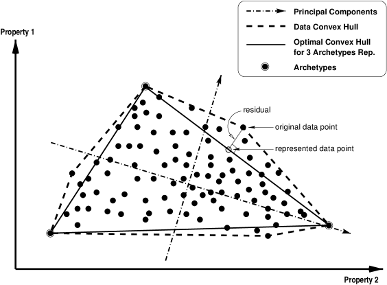
Figure 1: Diagrammatic comparison of archetypal analysis and PCA. The two dot-dashed axes illustrates the principal components of PCA. The dashed hexagon is the data convex hull, and the solid triangle shows the archetype convex hull for the case of three archetypes. Points lying within the archetype convex hull are represented exactly, while points lying outside are approximated by the nearest point on the archetype convex hull, as illustrated.

2.1 An exemplar

It is instructive to visualise the difference between archetypal analysis and PCA using an artificial two-dimensional (i.e. $m=2$) data set. Such a data set is exhibited as the points in Fig. 1. Using PCA, the data are represented by their projections (coordinates) referenced to principal components pointing in the two orthogonal directions of maximum data variance, illustrated as the dot-dashed axes. Because there are only two independent variables, two principal components will provide an exact reconstruction of every data point.

Archetypal analysis is a representation using basis vectors lying on the data convex hull. In Fig. 1 the dashed hexagon traces the data convex hull, like a rubber band stretched around the data set. The archetypal algorithm locates archetypes on this data convex hull that form (for the given number of archetypes) an optimal model of the convex hull. For example, if we represent the artificial data set with three archetypes, the archetypal algorithm determines 3 points on the data convex hull that outline a triangle, which is the archetype convex hull. Every data point within the triangle is exactly described (zero residual) by mixtures of the archetypes. Data points lying outside the triangle are represented as the nearest point on the triangle, as illustrated in Fig. 1. The distance between the original (external) data point and the represented data point is the residual. The sum of these residuals is minimized (expression 3) in the search for the optimal set of archetypes. For this particular data set, the data convex hull is a hexagon and six archetypes would provide an exact reconstruction of every data point.

There are three generic issues associated with archetypal analysis that are addressed in the following sections:

1. The quality of an archetypal representation of multi-dimensional data depends on the number of archetypes adopted. We demonstrate the outcome of using different numbers of archetypes.

2. Archetypes are located on the data convex hull and archetypal analysis is potentially sensitive to outliers. We investigate the effects of noise-generated outliers on archetypal analysis.

3. The input data set sometimes needs to be standardised before archetypal analysis. We discuss our experience in this respect.

3 Application to synthetic spectra

We apply archetypal analysis to study evolving star formation in model galaxies. We construct a set of spectra of model galaxies by assuming that each galaxy has experienced episodes of star formation with quasi-random amplitudes at past epochs. Motivated by the analysis of Reichardt et al. (2001), we model the galaxies as superpositions of stellar populations formed instantaneously, and now observed at ages of 0.007, 0.045, 0.3, 2 and 14 Gyr. The fiducial spectra at these ages are derived using the Pégase-II code of ?, adopting a ? initial mass function in the range [0.1,120] ${\rm M_{\odot}}$ and the stellar library of ?. Spectra were synthesised over the optical wavelength range 365 – 711 nm, with 2 nm spectral bins (174 bins). Since the shapes of the nebular emission lines are not predicted by Pégase-II we simulate them using Gaussians with a FWHM $\sim$ 5 nm. This treatment is not required for archetypal analysis, but allows convenient visual presentation.

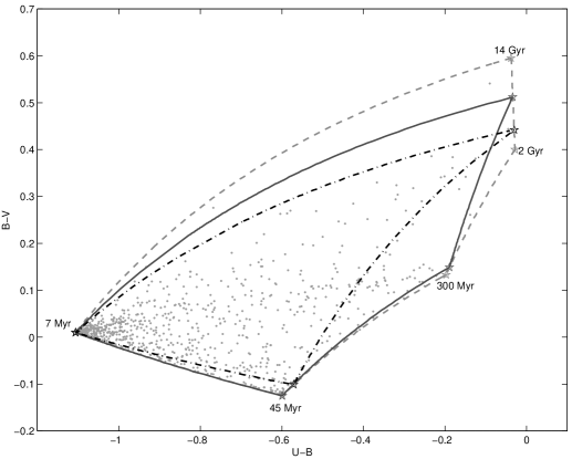
Figure 2: The projection of the data convex hull and the data themselves of a set of 900 noise free, composite spectra onto the two-colour $(B-V,U-B)$ plane. The dashed line outlines the data convex hull, the solid line shows the archetype convex hull for four archetypes, and the dot-dashed line shows the archetype convex hull for three archetypes.

To generate a model composite spectrum, the five fiducial spectra are first normalised to the same integrated flux. A composite spectrum is then generated via the superposition of fiducial spectra using a set of five quasi-random weighting factors. To satisfy the constraint that the sum of the five weighting factors be unity whist having quasi-uniform distribution, we generate the weighting factors according to the relationship $w_{i}={\rm U}[0,1](1-\sum_{n=1}^{i-1}w_{n})$, where ${\rm U}[0,1]$ denotes an uniformly distributed random number in [0,1]. Up to 5 random numbers are generated this way, or they are set to zero when $\sum_{n=1}^{i-1}w_{n}\geq 1$. These pseudo-random values are then randomly assigned as the five weighting factors. Since one of the five random values is never scaled, it retains an uniform distribution within [0,1] while the sum is constrained to be unity.

The sample of model galaxies is generated by repeating the process with different random numbers for each galaxy. In addition to determining the spectrum for each model galaxy, we also calculate the standard photometric colours. The distribution of the model galaxies in the two-colour $(B-V,U-B)$ plane is shown in Fig. 2. The fiducial spectra themselves are displayed in the first 5 panels across the top row of Fig. 3. The sixth panel exhibits an example of a composite spectrum, composed from ratios of 0.14, 0.66, 0.00, 0.13, and 0.08 of the fiducial spectra.

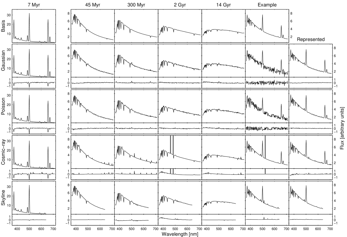
Figure 3: Top row: Fiducial spectra (columns 1-5), with a sample composite spectrum (column 6). Rows 2-4: Illustrating respectively the effects of model Gaussian (S/N=10), Poisson (S/N=10) and cosmic ray noise (5% random spikes), and night sky residual (with 5% amplitude) when five archetypes are used. In each row, columns 1-5 are the recovered archetypes, column 6 is the composite spectrum with its error, and column 7 is the represented composite spectrum. The small panels below rows 2-4 illustrate the differences between the spectrum immediately above, and the noise free counterpart in row 1.

 

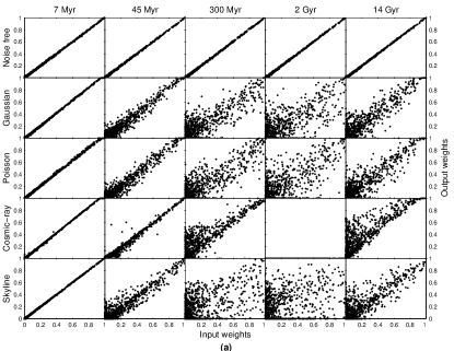
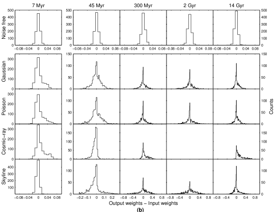
Figure 4: Correlations (a) and distributions (b) between the weights of the fiducial spectra in the 900 model spectra and the corresponding weights of the data represented by 5 archetypes. In both figures the five columns correspond to the five fiducial spectra (star formation episodes). Row 1: Noise free case; row 2: Gaussian noise added (S/N=10); row 3: Poisson noise added (S/N=10); row 4: cosmic ray added (5%); row 5: Skyline profile added ($\pm$5%).

Having generated sets of composite spectra we then apply archetypal analysis. Sample sizes of 50, 100 and 900 composite spectra have been explored. They show comparable results, and we present only the analysis of 900 composite spectra.

3.1 The number of archetypes

We first explore the use of different numbers of archetypes. To illustrate the key results, Fig. 2 shows a cloud of data points corresponding to 900 composite spectra projected onto the $(B-V,U-B)$ two-colour plane.

The corresponding projections of the five fiducial spectra are also shown. These are identical, to machine precision, to the projections of the archetypes when five archetypes are used. The projection of the archetype convex hull on the two-colour plane can be determined by noting that each edge of this polytope is a mixture of the archetypes lying at either end, with no contribution from the other three archetypes. The dashed line traces this projection of the 5-archetype convex hull. Its curvature arises from the non-linear relationship between spectral energy distribution and colour.

When four archetypes are used to represent the data, two of the archetypes remained essentially unchanged (7 Myr and 45 Myr) while the other two are mixtures of the three remaining fiducial spectra in the forms 81% 300 Myr + 19% 2 Gyr and 14% 2 Gyr + 85% 14 Gyr. When three archetypes are used, the 7 Myr fiducial spectrum is recovered, while the other two are the intermediate representations 80% 45 Myr + 20% 300 Myr and 44% 2 Gyr + 56% 14 Gyr. The four archetype and three archetype representations produce the archetype convex hulls shown as projections in Fig. 2.

In summary, the use of 5 archetypes recovers exactly the 5 fiducial spectra. When fewer archetypes are used, one or more of them represents the “younger” fiducial spectra with high purity, while the other archetypes appear as intermediate representations of the older fiducial spectra. This result is due primarily to the presence of prominent spectral features (especially emission lines) in the younger spectra, and the absence of marked differences between the older fiducial spectra.

3.2 Data representation in the presence of noise

Archetypal analysis is designed to focus attention on the outliers of the data set (?). This emphasis on outliers raises the question of sensitivity to noise, which potentially makes a larger contribution in the outliers of the data set. We examine this question in this section, showing that archetypal analysis is robust in the presence of the types of noise characterising astronomical spectroscopy.

We explore the effects of noise by adding four distinct kinds of contamination to the sample of 900 synthetic spectra described above. They are (i) random noise with Gaussian statistics, (ii) random noise with Poisson statistics, (iii) narrow, strong contamination dubbed “cosmic rays” and (iv) a pervasive fixed pattern dubbed “sky subtraction residual”.

The amplitude of the random noise models was selected to provide data with a characteristic signal-to-noise (S/N) ratio of 10. In particular, for Poisson random noise, the mean noise amplitude added to a any wavelength bin is determined from the flux of that wavelength bin. Here we have ignored sky spectrum contributions.

We simulated a 5% cosmic ray contamination rate, assuming Poisson statistics for the number of contaminating events per synthetic spectra. In this way, 44/900 spectra suffered single-pixel events, represented as a spike of three times the amplitude of the peak flux density in the corresponding spectrum. In one spectrum (1/900) two spikes were added. The wavelength of each spike was chosen at random.

Sky subtraction residuals were simulated using the sky spectral profile published by ?. In the analysis of real spectra, sky lines would be quasi-randomly redshifted relative to the galaxy lines, an effect we model by randomly blueshifting the sky-line spectrum with the range $0\leq z\leq 0.1$. The shifted sky spectra were rebinned in wavelength and scaled to represent random sky subtraction errors with relative amplitudes of $\pm 5\%$ (uniform distribution), and added to the synthetic spectra. The combination of random redshifts and wavelength rebinning reduces the wavelength span from 174 to 139 spectral bins.

Fig. 3 and Fig. 4 illustrate respectively the effects of noise on (a) the archetypes themselves, and (b) the coefficients that represent the data in terms of the archetypes. In Fig. 3, the first five panels of the top row display the fiducial spectra, which are essentially identical to the five archetypes found in the absence of noise. Beneath this row, each column shows the corresponding archetype derived from the contaminated data set, as well as a difference spectrum with respect to fiducial spectrum.

With the exception of the “2 Gyr, cosmic rays” case which is discussed below, there is an evident correlation between the “input” and “derived” weights, but there is also substantial scatter. Some of this scatter reflects the propagation of error into the archetypes themselves, although the recovered archetypes are generally quite similar to those derived in the absence of contamination. Most of the scatter arise from the propagation of error in fitting each spectrum as a mixture of archetypes. The appearance of large scatter for the “older” spectral components reflects the fact that the three “older” archetypes are similar to one another.

The rightmost panel in the top row of Fig. 3 illustrates one of the 900 synthetic spectra. In the column below, the corresponding contaminated synthetic spectra are exhibited, as well as the difference from the uncontaminated spectrum. The chosen spectrum is one that suffers a single cosmic ray event, in that form of contamination. To the right of these panels are the corresponding spectra obtained as the weighted sum of the archetypes. In all cases, the archetypal representation preserves spectral detail while reducing the amplitude of the contamination in the original spectrum. This result confirms the potential efficacy of archetypal analysis for compacting the size of a data set.

The results of archetypal analysis on the inferred statistical properties of the entire sample of 900 spectra is illustrated in Fig. 4. In part 4(a), each small panel is a scatter plot of points whose abscissa are the weights applied to the fiducial spectra in forming synthetic spectra, and whose ordinates are the derived weights of the corresponding archetypal representation. Deviations from perfect correlation reflect the propagation of errors due to contamination of the spectra into the inferred star formation history of each model galaxy. In Fig. 4(b), the corresponding distribution functions of the difference between the “input” and “derived” weight are exhibited.

The results illustrated in Fig. 4 reveal both the strengths and weaknesses of archetypal analysis. The tight correlations revealed in the top row reflect the essentially perfect correspondence between the fiducial spectra and the archetypes when uncontaminated data are analysed using five archetypes. The relatively tight correlations in the first two columns show that even in the presence of significant contamination, the spectral trace of “younger” populations can be measured with high precision. The distribution of points in the 300 Myr to 14 Gyr columns reflects the difficulty of extracting accurately the spectral trace of single, old star formation events in data having relatively poor S/N ratio. This problem is well understood, and the results are unlikely to be inferior to those that might derived from other methods.

It is illuminating to interpret these results in terms of the topology of the data and archetype convex hulls. The data can be regarded as 900 points (the number of spectra) in 174- (or 139-) dimensional (the number of wavelengths) space. When weak or moderate levels of Gaussian or Poisson noise are present, or a weak sky spectrum suffering random wavelength shifts are present, the data points including the vertices of the data convex hull are displaced by distances that are relatively small compared with their median distance from the origin. Consequently, the archetype convex hull differs only mildly from the corresponding archetype convex hull in the absence of contamination. The archetypes resemble those of the uncontaminated data, and because the number of archetypes is far smaller than the number of wavelengths, data representations are significantly smoothed.

The “2 Gyr, cosmic rays” panels in Fig. 3 and Fig. 4 are different from all other panels. In this case, archetypal analysis has derived as one of the archetypes a spectrum with two cosmic ray events in it. Because no other spectrum in the sample contains this pattern, the archetype does not contribute significantly to any of the data representations. The analysis thus yields results that closely approximate those that would be found were four archetypes used. This case illustrates the sensitivity of archetypal analysis to outliers with strong and unusual noise characteristics. However, it also shows that the method is robust even in the presence of such noise, and of course reveals a way to identify and excise noisy data in a systematic manner.

4 Prospects

In view of its emphasis on representing data sets as mixtures of pure types, archetypal analysis offers considerable promise in analysing galaxy spectra that are, presumably, superpositions of the spectra from different emission processes (AGN, nebulae, stars) and stellar populations of different ages. It provides near-perfect accuracy and precision in extracting star formation histories from noise-free synthetic data. The presence of noise, particularly with strongly non-Gaussian statistics, compromises this high accuracy but our studies suggest that the technique can be applied with success to galaxy spectral data with typical noise properties.

There are extensions to archetypal analysis that we have explored in a limited way. For example, the results of archetypal analysis depend to some extent on the pre-conditioning or standardisation of the input data. We found that with cosmic ray contamination, the best results are obtained when the data are standardised, while this seems unnecessary with Gaussian or Poisson random noise and for the sky subtraction residual set. We have shown that cosmic ray events may be effectively identified through their obvious presence in some archetypes. This invites exploration of an iterative approach to data conditioning in which non-physical components of the archetypes are progressively edited from the data set, providing a potentially powerful new methodology for peeling away contaminating components in the data. Archetypal analysis was designed to seek a representation using members of the data set. However, in some cases there are preferred models for the data. We have confirmed that Archetype Analysis is still applicable in this case, with the models replacing the archetypes. Used in this way, Archetypal Analysis shares many of the features of MOPED.

We are currently using archetypal analysis to analyse real galaxy spectra from the ? sample and the 2dFGRS survey (?).

References

- [Colless et al.¡2001¿] Colless M., et al. (the 2dFGRS team), 2001, MNRAS, 328, 1039.
- [Cutler & Breiman¡1994¿] Cutler A., Breiman L., 1994, Technometrics, 36, 338.
- [Fioc & Rocca-Volmerange¡1999¿] Fioc M., Rocca-Volmerange B., 1999, preprint (astro-ph/9912179).
- [Heavens, Jimenez & Lahav¡2000¿] Heavens A., Jimenez R., Lahav O., 2000, MNRAS, 317, 965.
- [Kennicutt¡1992¿] Kennicutt C.J., 1992, ApJSS, 79, 255.
- [Lahav¡2001¿] Lahav O., 2001, in Banday A.J., Zaroubi S., Bartelmann M., eds, Proc. MPA/ESO/MPE conference at Garching, Germany, 2000. Mining the Sky. Heidelberg: Springer-Verlag, p.33. Preprint (astro-ph/0012407).
- [Lejeune, Cuisinier & Buser¡1997; 1998¿] Lejeune T., Cuisinier F., Buser R., 1997, A&AS, 125, 229.
- [Lejeune, Cuisinier & Buser¡1997; 1998¿] Lejeune T., Cuisinier F., Buser R., 1998, A&AS, 130, 65.
- [Madgwick & Lahav¡2001¿] Madgwick D.S., Lahav O., 2001, in Treyer, Tresse, eds, Where’s the Matter? Tracing Dark and Bright Matter with the New Generation of Large Scale Surveys. Frontier Group. Preprint (astro-ph/0110220).
- [Murtagh & Heck¡1987¿] Murtagh F., Heck A., 1987, in Boyd R.L.F. et al., eds, Astrophysics and Space Science Library, Multivariate data analysis. D. Reidel Pub., Dordrecht, Holland, p.19.
- [Reichardt, Jimenez & Heavens¡2001¿] Reichardt C., Jimenez R., Heavens A, 2001, MNRAS, 327, 849.
- [Ronen et al.¡1999¿] Ronen S., Aragón-Salamanca A., Lahav O., 1999, MNRAS, 303, 284.
- [Salpeter¡1955¿] Salpeter E., 1955, ApJ, 121, 161.
- [Slonim et al.¡2001¿] Slonim N., Somerville R., Tishby N., Lahav O., 2001, MNRAS, 323, 270.