The Origin of the Heavy Elements: Recent Progress in
the Understanding of the $r$-Process

Abstract

There has been significant progress in the understanding of the $r$-process over the last ten years. The conditions required for this process have been examined in terms of the parameters for adiabatic expansion from high temperature and density. There have been many developments regarding core-collapse supernova and neutron star merger models of the $r$-process. Meteoritic data and observations of metal-poor stars have demonstrated the diversity of $r$-process sources. Stellar observations have also found some regularity in $r$-process abundance patterns and large dispersions in $r$-process abundances at low metallicities. This review summarizes the recent results from parametric studies, astrophysical models, and observational studies of the $r$-process. The interplay between nuclear physics and astrophysics is emphasized. Some suggestions for future theoretical, experimental, and observational studies of the $r$-process are given.

1 Introduction

The basic framework for understanding the origin of the elements was summarized in the classic works by Burbidge et al. [1] and Cameron [2] in 1957 (see [3] for a more up-to-date review). The crucial observational basis for developing this framework was the abundance distribution of stable and long-lived nuclei in the solar system. The slow ($s$) and the rapid ($r$) neutron-capture processes were proposed as the dominant mechanisms for producing the elements heavier than Fe. The nuclear systematics of these two processes provides a simple and beautiful explanation for the peaks at mass numbers $A=80$, 88, 130, 138, 195, and 208, respectively, in the solar abundance distribution (see Fig. 1). The work by Seeger et al. [5] in 1965 gave a comprehensive discussion of the $s$-process and the $r$-process based on the underlying nuclear physics. More recent reviews of the $s$-process can be found in [6]–[8]. This review focuses on the progress in the understanding of the $r$-process since the last major review by Cowan et al. [9] in 1991. After a basic introduction, the astrophysical conditions for a successful $r$-process are discussed in Sec. 2. Recent developments regarding core-collapse supernova and neutron star merger models of the $r$-process are reviewed in Sec. 3. Data from studies of meteorites and metal-poor stars and their implications for the $r$-process are discussed in Sec. 4. Some suggestions for future theoretical, experimental, and observational studies of the $r$-process are given in Sec. 5. For those readers who are interested in some particular aspects of the rich physics and astrophysics associated with the $r$-process, a good place to start is Sec. 5, where a brief summary is also provided. Together with the table of contents, this summary may serve as a guide in finding the topics of special interest that are covered here.

Figure 1: The logarithm of the solar abundances (normalized so that the elemental solar abundance of Si is $10^{6}$) as a function of mass number $A$. For clarity, only the abundances of the nuclei with even proton and neutron numbers are shown. When there are two or more stable nuclei with the same mass number, the abundance of the dominant isobar is shown. See [4] for the full set of abundances. The peaks at $A=80$, 88, 130, 138, 195, and 208 discussed in the text can be clearly seen (the abundance of ¹⁹⁵Pt, which defines the peak at $A=195$, is essentially the same as the abundance shown for $A=194$). It is interesting to note that the abundances of ¹¹⁸Sn and ¹²⁰Sn (with the magic proton number $Z=50$) are comparable to those in the peak at $A=130$.

1.1 The $s$-process

In the $s$-process, neutron capture is slow compared with $\beta$ decay so that an unstable nucleus produced by neutron capture $\beta$-decays to its stable daughter before it captures another neutron. Consequently, the $s$-process proceeds close to the $\beta$-stability line. The number of the stable nuclei with mass number $A$ produced in an $s$-process event, i.e., the yield $Y_{s}(A)$, is governed by

$$\dot{Y}_{s}(A)=\phi_{n}[\sigma_{n,\gamma}(A-1)Y_{s}(A-1)-\sigma_{n,\gamma}(A)Y_{s}(A)],$$ (1)

where $\dot{Y}_{s}(A)$ is the rate of change in $Y_{s}(A)$, $\phi_{n}$ is the neutron flux, and $\sigma_{n,\gamma}(A)$ is the neutron-capture cross section (appropriate for the conditions in the $s$-process environment) for the stable nucleus with mass number $A$. When an equilibrium is reached,

$$\sigma_{n,\gamma}(A-1)Y_{s}(A-1)=\sigma_{n,\gamma}(A)Y_{s}(A),$$ (2)

which means that the $s$-process yield of a stable nucleus is inversely proportional to its neutron-capture cross section. As the stable nuclei ⁸⁸Sr, ¹³⁸Ba, and ²⁰⁸Pb with the magic neutron numbers $N=50$, 82, and 126, respectively, have extremely small neutron-capture cross sections, the $s$-process produces abundance peaks at these nuclei, which are observed in the solar abundance distribution (see Fig. 1).

The $s$-process encounters the magic neutron numbers $N=50$, 82, and 126 at the stable nuclei with proton numbers $Z=38$, 56, and 82, respectively. As neutron capture is rapid compared with $\beta$ decay during the $r$-process, this process proceeds on the neutron-rich side of the $\beta$-stability line and encounters the same magic neutron numbers $N=50$, 82, and 126 at unstable neutron-rich progenitor nuclei with smaller proton numbers $Z\sim 30$, 48, and 69 corresponding to $A\sim 80$, 130, and 195, respectively. The production of these progenitor nuclei is favored by the $r$-process due to their relative stability associated with the magic neutron numbers. The successive $\beta$ decay of these nuclei following the cessation of rapid neutron capture then gives rise to the peaks at ⁸⁰Se, ¹³⁰Te, and ¹⁹⁵Pt observed in the solar abundance distribution (see Fig. 1).

It is useful to decompose the solar abundances into the separate contributions from the $s$-process and the $r$-process, respectively. This decomposition is trivial for the nuclei that can only be produced by the $s$-process or the $r$-process (i.e., the $s$-only or $r$-only nuclei). For example, the stable nucleus ¹³⁶Ba has a more neutron-rich stable isobar ¹³⁶Xe. The successive $\beta$ decay of the $r$-process progenitor nucleus with $A=136$ stops at ¹³⁶Xe and does not contribute to the abundance of ¹³⁶Ba. Thus, ¹³⁶Ba is an $s$-only nucleus. On the other hand, the unstable nucleus ¹²⁷Te is sandwiched by its two stable isotopes ¹²⁶Te and ¹²⁸Te. The $s$-process follows the $\beta$ decay of ¹²⁷Te and bypasses ¹²⁸Te. Thus, ¹²⁸Te is an $r$-only nucleus. In addition, as the region immediately beyond the heaviest stable nucleus ²⁰⁹Bi is populated by very short-lived nuclei, the long-lived nuclei beyond ²⁰⁹Bi such as ²³²Th, ²³⁵U, and ²³⁸U cannot be produced by the $s$-process and must be attributed to the $r$-process. Except for the $s$-only and $r$-only nuclei, a heavy nucleus generally receives contributions from both the $s$-process and the $r$-process. The decomposition of the solar abundances into the solar $s$-process and $r$-process abundances, respectively, can be accomplished by a phenomenological approach that is based on mostly nuclear physics and observational data or by a full approach that is based on nuclear physics, stellar physics, and Galactic chemical evolution. In both approaches, the goal is to calculate the solar $s$-process abundances directly from theory and then to obtain the solar $r$-process abundances by subtracting the $s$-process contributions from the total solar abundances.

The main nuclear physical input for the $s$-process is the neutron-capture cross sections. The astrophysical input is the intensity and the duration of the neutron flux in individual $s$-process events, which can be determined from stellar physics and Galactic chemical evolution in the full approach. In the phenomenological approach, the astrophysical input is parameterized as a distribution of the integrated exposure to the neutron flux. A given neutron-exposure distribution specifies a function

$$f_{s}(A)=\sigma_{n,\gamma}(A)N_{s}(A),$$ (3)

where $N_{s}(A)$ is the $s$-process abundance of the stable nucleus with mass number $A$ that is produced by this neutron-exposure distribution. The neutron-capture cross sections and the solar abundances of the $s$-only nuclei in different mass regions can be used to select the neutron-exposure distribution that gives the function $f_{\odot,s}(A)$ as defined in Eq. (3) but for the solar $s$-process abundance $N_{\odot,s}(A)$. The solar $r$-process abundance $N_{\odot,r}(A)$ can then be obtained as

$$N_{\odot,r}(A)=N_{\odot}(A)-N_{\odot,s}(A)=N_{\odot}(A)-[f_{\odot,s}(A)/\sigma_{n,\gamma}(A)],$$ (4)

where $N_{\odot}(A)$ is the total solar abundance of the stable nucleus with mass number $A$. Figure 2a shows the solar $r$-process abundances calculated from this phenomenological approach by Arlandini et al. [10].

Figure 2: The logarithm of the solar $r$-process abundances (normalized so that the elemental solar abundance of Si is $10^{6}$) as a function of mass number $A$. These abundances are obtained by subtracting the $s$-process contributions calculated from (a) the phenomenological approach and (b) models of two AGB stars. See [10] for details.

Clearly, the solar $r$-process abundances obtained above are subject to possibly large uncertainties when the solar $s$-process fraction $\beta_{\odot,s}(A)=N_{\odot,s}(A)/N_{\odot}(A)$ is close to unity. For example, the phenomenological approach gives $\beta_{\odot,s}(^{139}{\rm La})=0.83$ while stellar-model calculations (see below) give $\beta_{\odot,s}(^{139}{\rm La})=0.62$ [10]. This difference indicates that the uncertainty in the solar $r$-process abundance of ¹³⁹La may be as large as a factor of 2.2. An important issue is then the accuracy of the solar $s$-process abundances as calculated from the phenomenological approach. The systematic error of this approach can only be assessed by the full approach that calculates and incorporates the $s$-process yields in different astrophysical environments over the Galactic history prior to the formation of the solar system. The phenomenological approach has identified a weak $s$-process, which produces the nuclei up to ⁸⁸Sr, and a main $s$-process, which produces the nuclei ⁸⁸Sr and above. The weak $s$-process occurs in massive stars while the main $s$-process occurs in low-mass asymptotic giant branch (AGB) stars (e.g., [6]). Arlandini et al. [10] calculated the $s$-process yields of two AGB stars with a metallicity of half the solar value but with masses of $1.5\,M_{\odot}$ and $3\,M_{\odot}$ ($M_{\odot}$ being the mass of the sun), respectively. It is encouraging that the main component of the solar $s$-process abundances as calculated from the phenomenological approach can be essentially reproduced by averaging the $s$-process yields of these two stars (see Fig. 2b). However, this should be viewed only as a significant step towards checking and correcting the phenomenological results by the full approach. In using the solar $r$-process abundances obtained by subtracting the $s$-process contributions as calculated from the phenomenological approach or a few sample stellar models, it is important to recognize that these results are generally reliable when $\beta_{\odot,s}(A)$ is small, but may have substantial uncertainties when $\beta_{\odot,s}(A)$ is close to unity. In addition, the solar $r$-process abundances at $A=206$–209 shown in Fig. 2 may have to be significantly revised due to important contributions from low-metallicity AGB stars [11].

Another potential problem with the solar $r$-process abundances obtained by subtracting the $s$-process contributions is that some nuclei may be produced by processes other than the $s$-process and the $r$-process. The small contributions from the so-called “$p$-process” were considered in [6]. However, it is rather difficult to estimate the contributions to the solar abundances of the nuclei above the Fe group but with $A\>\lower 1.72218pt\hbox{$\stackrel{{\scriptstyle\scriptstyle<}}{{\scriptstyle\sim}}$}\>90$ that may come from the $\alpha$-process to be discussed in Sec. 2.3. In view of this difficulty, the solar “$r$-process” abundances at $A<88$ with a peak at $A=80$ (possibly corresponding to the progenitor nuclei with $N=50$) will not be discussed here.

1.2 The $r$-process

The pattern of the solar $r$-process abundances (the solar $r$-pattern) obtained in connection with the $s$-process studies has played an essential role in the understanding of the $r$-process. As mentioned in Sec. 1.1, the peaks at $A=130$ and 195 in this pattern can be accounted for by the nuclear properties associated with the magic neutron numbers $N=82$ and 126, respectively. It is convenient to consider the nuclear physical aspects of the $r$-process separately from the astrophysical aspects that treat the conditions in the $r$-process environment. Provided that an $r$-process occurs, the resulting yield pattern is mostly determined by the nuclear systematics of the interplay between neutron capture, photo-disintegration, $\beta$ decay, and possibly fission. For the nuclei with proton numbers $Z<80$, fission may be ignored. Then the number of the nuclei $(Z,A)$ with proton number $Z$ and mass number $A$ produced in an $r$-process event, i.e., the yield $Y(Z,A)$, is governed by

$$\dot{Y}(Z,A) = n_{n}\langle v\sigma_{n,\gamma}(Z,A-1)\rangle Y(Z,A-1)+\lambda_{\gamma,n}(Z,A+1)Y(Z,A+1)+\lambda_{\beta 0}(Z-1,A)Y(Z-1,A)$$ (5)

$$+\lambda_{\beta 1}(Z-1,A+1)Y(Z-1,A+1)+\lambda_{\beta 2}(Z-1,A+2)Y(Z-1,A+2)$$

$$+\lambda_{\beta 3}(Z-1,A+3)Y(Z-1,A+3)-n_{n}\langle v\sigma_{n,\gamma}(Z,A)\rangle Y(Z,A)-\lambda_{\gamma,n}(Z,A)Y(Z,A)$$

$$-[\lambda_{\beta 0}(Z,A)+\lambda_{\beta 1}(Z,A)+\lambda_{\beta 2}(Z,A)+\lambda_{\beta 3}(Z,A)]Y(Z,A),$$

where $n_{n}$ is the neutron number density, $n_{n}\langle v\sigma_{n,\gamma}(Z,A)\rangle$ is the thermally averaged neutron-capture rate, $\lambda_{\gamma,n}(Z,A)$ is the photo-disintegration rate, and $\lambda_{\beta 0}(Z,A)$, $\lambda_{\beta 1}(Z,A)$, $\lambda_{\beta 2}(Z,A)$, and $\lambda_{\beta 3}(Z,A)$ are the rates for $\beta$ decay followed by emission of 0, 1, 2, and 3 neutrons, respectively. Equation (5) and the like form an $r$-process reaction network. Some approximations that are either helpful in understanding the results from full network calculations or used in place of such calculations are discussed below.

1.2.1 $(n,\gamma)\rightleftharpoons(\gamma,n)$ equilibrium

When both neutron capture and photo-disintegration occur much faster than $\beta$ decay, a statistical $(n,\gamma)\rightleftharpoons(\gamma,n)$ equilibrium is achieved and the yields $Y(Z,A)$ and $Y(Z,A+1)$ of two neighboring isotopes satisfy

$${Y(Z,A+1)\over Y(Z,A)}={n_{n}\langle v\sigma_{n,\gamma}(Z,A)\rangle\over\lambda_{\gamma,n}(Z,A+1)}=n_{n}\left({2\pi\hbar^{2}\over m_{u}kT}\right)^{3/2}\left({A+1\over A}\right)^{3/2}{G(Z,A+1)\over 2G(Z,A)}\exp\left[{S_{n}(Z,A+1)\over kT}\right],$$ (6)

where $T$ is the temperature, $\hbar$ is the Planck constant, $k$ is the Boltzmann constant, $m_{u}$ is the atomic mass unit, $G(Z,A)$ is the nuclear partition function, and $S_{n}(Z,A+1)$ is the neutron separation energy. The most abundant isotope in the isotopic chain of $Z$ has a neutron separation energy of

$$S_{n}^{0} \approx kT\ln\left[{2\over n_{n}}\left({m_{u}kT\over 2\pi\hbar^{2}}\right)^{3/2}\right]$$ (7)

$$= \left({T\over 10^{9}\ {\rm K}}\right)\left\{2.79+0.198\left[\log\left({10^{20}\ {\rm cm}^{-3}\over n_{n}}\right)+{3\over 2}\log\left({T\over 10^{9}\ {\rm K}}\right)\right]\right\}\ {\rm MeV},$$

which can be seen from Eq. (6) by setting $Y(Z,A+1)\approx Y(Z,A)$ and neglecting the relatively small differences in the nuclear partition function and the mass number. As $S_{n}^{0}$ only depends on $n_{n}$ and $T$, the most abundant isotopes in different isotopic chains have approximately the same neutron separation energy, which is $\sim 2$–3 MeV for typical conditions during the $r$-process. Due to the odd-even effect caused by pairing, the most abundant isotope always has an even $N$. For this reason, it may be more appropriate to characterize the most abundant isotope in the isotopic chain of $Z$ by a two-neutron separation energy $S_{2n}(Z,A+2)=S_{n}(Z,A+2)+S_{n}(Z,A+1)\approx 2S_{n}^{0}$ [12].

The conditions for $(n,\gamma)\rightleftharpoons(\gamma,n)$ equilibrium were first examined in [13] based on steady-flow calculations (see Sec. 1.2.2) and were found to be $T\>\lower 1.72218pt\hbox{$\stackrel{{\scriptstyle\scriptstyle>}}{{\scriptstyle\sim}}$}\>2\times 10^{9}$ K and $n_{n}\>\lower 1.72218pt\hbox{$\stackrel{{\scriptstyle\scriptstyle>}}{{\scriptstyle\sim}}$}\>10^{20}$ cm^-3. Later studies [14, 15] emphasized the effects of the nuclear physical input, such as the masses of neutron-rich nuclei far from stability, on the conditions for $(n,\gamma)\rightleftharpoons(\gamma,n)$ equilibrium. Essentially all of the nuclear physical input for the $r$-process is calculated from theory (see [9] for a review) and different calculations sometimes give very different results (e.g., [12, 14, 15]). The uncertainties in the theoretical results can be reduced by making use of the existing but limited experimental knowledge on neutron-rich nuclei far from stability (e.g., [16]). Based on full network calculations with two different sets of nuclear physical input, it was found that $(n,\gamma)\rightleftharpoons(\gamma,n)$ equilibrium is obtained for $n_{n}\>\lower 1.72218pt\hbox{$\stackrel{{\scriptstyle\scriptstyle>}}{{\scriptstyle\sim}}$}\>10^{20}$ cm^-3 at $T=2\times 10^{9}$ K and for $n_{n}\>\lower 1.72218pt\hbox{$\stackrel{{\scriptstyle\scriptstyle>}}{{\scriptstyle\sim}}$}\>10^{28}$ cm^-3 at $T=10^{9}$ K [15]. In general, the higher the temperature and the neutron number density are, the better $(n,\gamma)\rightleftharpoons(\gamma,n)$ equilibrium holds.

1.2.2 steady flow and steady $\beta$-flow

In a steady flow, $\dot{Y}(Z,A)=0$ for all the nuclei in the reaction network and the yields of these nuclei are determined by a system of linear algebraic equations. Sample steady-flow $r$-process calculations can be found in [17]. The steady-flow solution also satisfies

$$\lambda_{\beta}(Z-1)Y(Z-1)=\lambda_{\beta}(Z)Y(Z),$$ (8)

where $Y(Z)=\sum_{A}Y(Z,A)$ and $\lambda_{\beta}(Z)=\sum_{A}\lambda_{\beta}(Z,A)Y(Z,A)/Y(Z)$ with $\lambda_{\beta}(Z,A)$ being the total $\beta$-decay rate of the nucleus $(Z,A)$. A special case of the steady flow arises when the $r$-process is also in $(n,\gamma)\rightleftharpoons(\gamma,n)$ equilibrium. In this case, essentially all the abundance in an isotopic chain is carried by one or two isotopes with $S_{2n}\sim 2S_{n}^{0}$ (see Sec. 1.2.1). Such isotopes are called the waiting-point nuclei as the $r$-process must wait for their $\beta$ decay in order to produce the nuclei in the next isotopic chain. The above special case of the steady flow is called the steady $\beta$-flow. As can be seen from Eq. (8), the yield of a waiting-point nucleus in a steady $\beta$-flow is inversely proportional to its $\beta$-decay rate.

A true steady flow requires that nuclei be fed into the reaction network from below for a sufficiently long time. The results from a steady-flow calculation are valid only for certain regions of the network where this condition is met. It was found that a steady $\beta$-flow may be obtained for the waiting-point nuclei between two magic neutron numbers, e.g., those with $50<N\leq 82$ [18]. If steady $\beta$-flows are realized in the $r$-process, then the peaks at $A=130$ and 195 in the solar $r$-pattern can be attributed to the extremely small $\beta$-decay rates of the waiting-point nuclei with the magic neutron numbers $N=82$ and 126, respectively.

1.2.3 fission cycling

If the $r$-process involves progenitor nuclei with $Z\geq 80$, then fission should be included in the reaction network. This may lead to fission cycling, a scenario where the heaviest nucleus produced by the $r$-process fissions and a cyclic flow occurs between this nucleus and its fission fragments in the presence of a large neutron abundance. Consider a simple example where $(n,\gamma)\rightleftharpoons(\gamma,n)$ equilibrium holds and fission occurs upon the $\beta$ decay of the heaviest waiting-point nucleus with proton number $Z_{f}$, which produces two fragments with fixed proton numbers $Z_{1}$ and $Z_{2}$ ($Z_{2}>Z_{1}$), respectively. A sufficiently long time after the onset of the $r$-process, the nuclei with $Z<Z_{1}$ are depleted to negligible abundances by neutron capture and $\beta$ decay. Then the yields of the waiting-point nuclei involved in fission cycling are governed by

$$\dot{Y}(Z)=\lambda_{\beta}(Z-1)Y(Z-1)-\lambda_{\beta}(Z)Y(Z)$$ (9)

for $Z_{1}<Z<Z_{2}$ and $Z_{2}<Z\leq Z_{f}$, and

$$\dot{Y}(Z_{1}) = \lambda_{\beta}(Z_{f})Y(Z_{f})-\lambda_{\beta}(Z_{1})Y(Z_{1}),$$ (10)

$$\dot{Y}(Z_{2}) = \lambda_{\beta}(Z_{f})Y(Z_{f})+\lambda_{\beta}(Z_{2}-1)Y(Z_{2}-1)-\lambda_{\beta}(Z_{2})Y(Z_{2}).$$ (11)

With feeding of the nuclear flow at the lower proton numbers $Z_{1}$ and $Z_{2}$ by fission, a steady state can be obtained after a few fission cycles. This results in a rather robust yield pattern with peaks at $A\sim 130$ and 195 [5].

1.2.4 freeze-out

In an $r$-process event, the neutron number density and the temperature decrease with time. Neutron capture ceases to be efficient and the $r$-process freezes out when

$$n_{n}\langle v\sigma_{n,\gamma}\rangle\tau\sim 1,$$ (12)

where $\tau$ is the timescale over which $n_{n}$ decreases significantly. The freeze-out may involve several stages during which the approximations discussed above are most likely to break down. Here full network calculations are especially important. After the freeze-out, the progenitor nuclei successively $\beta$-decay towards stability. In particular, the progenitor nuclei with magic neutron numbers, which are in the peaks of the $r$-process yield pattern at the freeze-out, $\beta$-decay to the stable nuclei with approximately the same mass numbers but with smaller nonmagic neutron numbers. The freeze-out pattern may differ significantly from the final yield pattern due to modifications by processes such as $\beta$-delayed neutron emission after the freeze-out.

2 Astrophysical Conditions for the $r$-Process

The photo-disintegration rate $\lambda_{\gamma,n}(Z,A+1)$ is related to the neutron-capture rate $n_{n}\langle v\sigma_{n,\gamma}(Z,A)\rangle$ through detailed balance, which leads to Eq. (6) for $(n,\gamma)\rightleftharpoons(\gamma,n)$ equilibrium. The specification of the rates for neutron capture and photo-disintegration in the $r$-process network requires the neutron number density $n_{n}$ and the temperature $T$. In traditional calculations (e.g., [12, 14, 15, 18]), a seed nucleus, usually ⁵⁶Fe, is irradiated with neutrons at constant values of $n_{n}$ and $T$ for a time $t_{\rm irr}$. The final yield pattern is then obtained by assuming an instantaneous freeze-out and taking into account the modifications of the freeze-out pattern due to $\beta$-delayed neutron emission. Such calculations showed that the solar $r$-pattern must be accounted for by a superposition of the yield patterns resulting from distinct sets of $n_{n}$, $T$, and $t_{\rm irr}$. These sets of parameters with typical values of $n_{n}>10^{20}$ cm^-3, $T\sim 10^{9}$ K, and $t_{\rm irr}\>\lower 1.72218pt\hbox{$\stackrel{{\scriptstyle\scriptstyle>}}{{\scriptstyle\sim}}$}\>1$ s were considered to represent the astrophysical conditions in the $r$-process events that occurred over the Galactic history prior to the formation of the solar system.

In a realistic $r$-process event, $n_{n}$ and $T$ decrease with time. The new feature of an $r$-process calculation taking this into account can be illustrated by considering the phase during which $(n,\gamma)\rightleftharpoons(\gamma,n)$ equilibrium holds. Due to the evolution of $n_{n}$ and $T$, the waiting-point nucleus with mass number $A_{\rm WP}$ in the isotopic chain of $Z$ changes with time $t$, which introduces a time dependence into the effective $\beta$-decay rate $\lambda_{\beta}(Z,t)=\sum_{A}\lambda_{\beta}(Z,A)Y(Z,A)/Y(Z)\approx\lambda_{\beta}[Z,A_{\rm WP}(t)]$. As $\lambda_{\beta}[Z,A_{\rm WP}(t)]$ tends to be very large at early times when high values of $n_{n}$ favor the waiting-point nuclei close to the neutron-drip line, the duration of an $r$-process can be greatly reduced. By contrast, the waiting-point nuclei and the effective $\beta$-decay rates do not change in the traditional $r$-process calculations when $(n,\gamma)\rightleftharpoons(\gamma,n)$ equilibrium is assumed. Thus, the neutron irradiation time $t_{\rm irr}$ used in the traditional calculations to obtain the solar $r$-pattern may be much longer than the actual timescale for an $r$-process. It is also clear that the decrease of $n_{n}$ and $T$ in an $r$-process event causes $(n,\gamma)\rightleftharpoons(\gamma,n)$ equilibrium to break down eventually and makes the freeze-out more like a multi-stage process rather than a sudden one.

The evolution of $n_{n}$ in an $r$-process event can be described in terms of the neutron-to-seed ratio

$$R_{n/s}(t)=Y_{n}(t)/Y_{s}(t_{0}),$$ (13)

where $Y_{n}(t)$ is the neutron abundance at time $t$ and $Y_{s}(t_{0})$ is the initial abundance of seed nuclei. If fission can be ignored, conservation of mass and the total number of nuclei gives

$$Y_{n}(t)+\sum_{(Z,A)}AY(Z,A) = Y_{n}(t_{0})+A_{s}Y_{s}(t_{0}),$$ (14)

$$\sum_{(Z,A)}Y(Z,A) = Y_{s}(t_{0}),$$ (15)

where $A_{s}$ is the mass number of the seed nucleus and the sums extend over all the nuclei with $A\geq A_{s}$. Equations (14) and (15) can be rewritten as

$$\bar{A}(t)+R_{n/s}(t)=A_{s}+R_{n/s}(t_{0}),$$ (16)

where $\bar{A}(t)=\sum_{(Z,A)}AY(Z,A)/\sum_{(Z,A)}Y(Z,A)$ is the average mass number of the nuclei with $A\geq A_{s}$ that are in the $r$-process network at time $t$. In general, when the $r$-process freezes out at $t=t_{\rm FO}$, $R_{n/s}(t_{\rm FO})\>\lower 1.72218pt\hbox{$\stackrel{{\scriptstyle\scriptstyle<}}{{\scriptstyle\sim}}$}\>1$ and $\bar{A}(t_{\rm FO})\approx A_{s}+R_{n/s}(t_{0})$. Thus, the outcome of an $r$-process event can be simply estimated from the initial neutron-to-seed ratio and the mass number of the seed nucleus.

The initial neutron-to-seed ratio $R_{n/s}(t_{0})$ not only provides a convenient means to characterize an $r$-process event but also highlights two important issues: where do the seed nuclei come from and how is $R_{n/s}(t_{0})$ determined? Observations of metal-poor stars to be discussed in Sec. 4 showed that the $r$-process already occurred in the early history of the Galaxy. This suggests that an $r$-process event cannot rely on some previous astrophysical events to provide the seed nuclei and must produce the seed nuclei within the event itself. The production of the seed nuclei and the determination of $R_{n/s}(t_{0})$ in an $r$-process event can be illustrated by considering a rather generic scenario in which neutron-rich material adiabatically expands from high temperature and density. The parameters characterizing the expansion that results in a successful $r$-process can be taken as a new measure of the astrophysical conditions for the $r$-process.

2.1 Adiabatic expansion from high temperature and density

The astrophysical input for a nucleosynthesis calculation includes the initial state and the time evolution of temperature and density. For electrically-neutral matter expanding from $T\>\lower 1.72218pt\hbox{$\stackrel{{\scriptstyle\scriptstyle>}}{{\scriptstyle\sim}}$}\>10^{10}$ K, the initial nuclear composition is

$$Y_{p}(0) = Y_{e},$$ (17)

$$Y_{n}(0) = 1-Y_{e},$$ (18)

where $Y_{e}$ is the net electron number per baryon, or the electron fraction. Neutron-rich matter has $Y_{e}<0.5$. For adiabatic expansion, the thermodynamic evolution of the matter is governed by

$$TdS+\sum_{(Z,A)}\mu(Z,A)dY(Z,A)=0,$$ (19)

where $S$ is the total entropy per baryon for all the particles in the matter (nucleons, nuclei, $e^{-}$, $e^{+}$, and photons) and $\mu(Z,A)$ is the chemical potential (including the rest mass) of the nucleus $(Z,A)$. At $T\>\lower 1.72218pt\hbox{$\stackrel{{\scriptstyle\scriptstyle>}}{{\scriptstyle\sim}}$}\>6\times 10^{9}$ K (usually also corresponding to high density), the forward strong and electromagnetic reactions are balanced by their reverse reactions. This results in nuclear statistical equilibrium (NSE), for which the second term on the left-hand side of Eq. (19) vanishes and the adiabatic condition reduces to $S$ being constant. After NSE breaks down, some entropy is generated by out-of-equilibrium reactions. However, this has little effect on considerations of the $r$-process [19]. So $S$ may be taken as constant during adiabatic expansion.

If photons are much more abundant than nucleons and nuclei (radiation dominance, $S\gg 10$ in units of $k$ per baryon),

$$S\approx{11\pi^{2}\over 45}\left({kT\over\hbar c}\right)^{3}{m_{u}\over\rho}=3.34\left({T\over 10^{9}\ {\rm K}}\right)^{3}\left({10^{5}\ {\rm g\ cm}^{-3}\over\rho}\right)$$ (20)

for $T\>\lower 1.72218pt\hbox{$\stackrel{{\scriptstyle\scriptstyle>}}{{\scriptstyle\sim}}$}\>5\times 10^{9}$ K when $e^{-}$ and $e^{+}$ are also abundant. In Eq. (20), $\rho$ is the matter density. The coefficient 3.34 in Eq. (20) should be replaced by smaller values for $T<5\times 10^{9}$ K due to the annihilation of $e^{-}$ and $e^{+}$ (e.g., the proper coefficient is 1.21 for $T\>\lower 1.72218pt\hbox{$\stackrel{{\scriptstyle\scriptstyle<}}{{\scriptstyle\sim}}$}\>10^{9}$ K). On the other hand, if nucleons and nuclei are much more abundant than photons (matter dominance, $S\>\lower 1.72218pt\hbox{$\stackrel{{\scriptstyle\scriptstyle<}}{{\scriptstyle\sim}}$}\>10$), $S$ depends on $T$ and $\rho$ as $\ln(T^{3/2}/\rho)$. In general, $S$ provides a relation between $T$ and $\rho$ during adiabatic expansion. So only the time evolution of $T$ or $\rho$ needs to be specified explicitly for a nucleosynthesis calculation. One of the parametrizations used in the literature ([20], but see [19, 21] for different choices) is

$$T(t)=T(0)\exp\left(-{t/\tau_{\rm dyn}}\right),$$ (21)

where $\tau_{\rm dyn}$ is the dynamic timescale of the expansion. Thus, a nucleosynthesis calculation can be done for matter adiabatically expanding from e.g., $T\sim 10^{10}$ K once the parameters $Y_{e}$, $S$, and $\tau_{\rm dyn}$ are given.

2.2 Statistical equilibrium and nucleosynthesis

In NSE, the abundance of the nucleus $(Z,A)$ can be obtained from $\mu(Z,A)=Z\mu_{p}+(A-Z)\mu_{n}$ as

$$Y(Z,A)={G(Z,A)A^{3/2}\over 2^{A}}\left({2\pi\hbar^{2}\over m_{u}kT}\right)^{3(A-1)/2}\left({\rho\over m_{u}}\right)^{A-1}Y_{n}^{A-Z}Y_{p}^{Z}\exp\left[{B(Z,A)\over kT}\right],$$ (22)

where $B(Z,A)$ is the nuclear binding energy of the nucleus $(Z,A)$. The nuclear composition in NSE does not depend on the reaction rates and is completely specified by $Y_{e}$, $T$, and $\rho$ together with the constraints of charge and mass conservation:

$$Y_{e} = Y_{p}+\sum_{(Z,A)}ZY(Z,A),$$ (23)

$$1 = Y_{n}+Y_{p}+\sum_{(Z,A)}AY(Z,A),$$ (24)

where the sums over nuclei exclude the nucleons. After NSE breaks down at $T\sim 6\times 10^{9}$ K, the nuclear composition is governed by the development of quasi-equilibrium (QSE) clusters. The total abundance in each QSE cluster is specified by the rates for the nuclear flows into and out of the cluster, but the relative abundances of the nuclei within the cluster are the same as given by Eq. (22) and again do not depend on the reaction rates [22, 23]. A familiar example of QSE is $(n,\gamma)\rightleftharpoons(\gamma,n)$ equilibrium, for which each isotopic chain is a QSE cluster. The total abundance $Y(Z)$ in the isotopic chain of $Z$ is determined by the $\beta$ decay of the nuclei in the isotopic chains of $Z-1$ and $Z$, but the abundance ratio $Y(Z,A+1)/Y(Z,A)$ as given in Eq. (6) can be simply obtained from Eq. (22).

At $6\times 10^{9}\ {\rm K}\>\lower 1.72218pt\hbox{$\stackrel{{\scriptstyle\scriptstyle>}}{{\scriptstyle\sim}}$}\>T\>\lower 1.72218pt\hbox{$\stackrel{{\scriptstyle\scriptstyle>}}{{\scriptstyle\sim}}$}\>4\times 10^{9}\ {\rm K}$, there are two major QSE clusters: the light one involving neutrons, protons, and $\alpha$-particles, and the heavy one involving ¹²C and heavier nuclei [23]. The abundance of $\alpha$-particles in the light cluster is given by Eq. (22) while the relative abundances of the nuclei within the heavy cluster can be estimated by using the same equation. The total abundance in the heavy cluster is governed by the net flow out of the light one, which crucially depends on the reactions $3\alpha\to{{}^{12}{\rm C}}+\gamma$, $\alpha+\alpha+n\to{{}^{9}{\rm Be}}+\gamma$ followed by $\alpha+{{}^{9}{\rm Be}}\to{{}^{12}{\rm C}}+n$, and all the reverse reactions. The nuclear composition of the heavy cluster freezes out at $T\sim 4\times 10^{9}$ K. This composition is slightly modified by capture of neutrons and $\alpha$-particles down to $T\sim 2\times 10^{9}$ K, at which temperature essentially all charged-particle reactions freeze out due to the Coulomb barrier. If there is a sufficiently high neutron abundance at this point, $(n,\gamma)\rightleftharpoons(\gamma,n)$ equilibrium takes over and an $r$-process starts.

2.3 Determination of the initial neutron-to-seed ratio

As neutron-rich matter with $Y_{p}(0)=Y_{e}<0.5$ and $Y_{n}(0)=1-Y_{e}$ adiabatically expands from $T\sim 10^{10}$ K, its nuclear composition evolves as follows based on the discussion in Sec. 2.2. The first phase of evolution is in NSE, during which essentially all the protons are assembled into $\alpha$-particles. When NSE breaks down at $T\sim 6\times 10^{9}$ K, the nuclear composition is dominated by neutrons and $\alpha$-particles. During the subsequent phase of evolution in QSE, heavy nuclei are produced subject to the influence of the bottle-neck imposed by the three-body reactions $3\alpha\to{{}^{12}{\rm C}}+\gamma$ and $\alpha+\alpha+n\to{{}^{9}{\rm Be}}+\gamma$ that connect the light QSE cluster and the heavy one. The overall neutron excess $\eta=1-2Y_{e}$ is crucial to the composition of the heavy QSE cluster. For $0<\eta<0.05$ that is similar to the neutron excess $\eta(Z,A)=1-(2Z/A)$ of the individual nuclei in the Fe group, these nuclei are the heavy nuclei favored by QSE as they have the largest nuclear binding energy per nucleon $B(Z,A)/A$. By contrast, QSE favors the heavy nuclei with $Z\sim 35$–40 and $A\sim 90$ (close to the magic neutron number $N=50$) for $\eta>0.05$. These nuclei have much larger values of $\eta(Z,A)$ but similar values of $B(Z,A)/A$ compared with the Fe group nuclei. The overall $\eta$ required for producing the heavy nuclei with $Z\sim 35$–40 and $A\sim 90$ can be significantly smaller than the values of $\eta(Z,A)\sim 0.1$–0.2 for these nuclei if the abundance $Y_{\alpha}$ of $\alpha$-particles is large. This is because $\eta\approx X_{n}+\sum_{(Z,A)}\eta(Z,A)X(Z,A)$ with $X_{n}$ and $X(Z,A)$ being the mass fractions of neutrons and nuclei, respectively. The $\alpha$-particles have no neutron excess and their presence allows $\eta$ to be small by reducing the mass fraction of the heavy nuclei that have significant neutron excess. The composition of the heavy nuclei freezes out of QSE at $T\sim 4\times 10^{9}$ K and is modified somewhat by capture of neutrons and $\alpha$-particles down to $T\sim 2\times 10^{9}$ K. Thereafter, an $r$-process occurs as the heavy nuclei with $Z\sim 35$–40 and $A\sim 90$ become the seed nuclei to capture the remaining neutrons. The production of heavy nuclei in the presence of significant neutron and $\alpha$-particle abundances was first proposed as the precursor to the $r$-process by Woosley and Hoffman [24], who referred to this as the “$\alpha$-process.” A thermodynamic approach to understand this process was given in [23].

For clarity in discussing adiabatic expansion of neutron-rich matter, the beginning of the expansion is denoted as $t=0$, that of the $\alpha$-process is denoted as $t_{\alpha}$, and that of the $r$-process is denoted as $t_{0}$. The initial neutron-to-seed ratio $R_{n/s}(t_{0})$ for the $r$-process is determined by the abundances of neutrons and heavy nuclei at the end of the $\alpha$-process, which in turn depend on the net flow into the heavy QSE cluster from the light one during the $\alpha$-process. As discussed in Sec. 2.2, this flow starts with the reactions building ¹²C. The physics involved in the determination of $R_{n/s}(t_{0})$ is reflected by the dependence of $R_{n/s}(t_{0})$ on $Y_{e}$, $S$, and $\tau_{\rm dyn}$, and can be illustrated by focusing on the reactions $\alpha+\alpha+n\to{{}^{9}{\rm Be}}+\gamma$ and $\alpha+{{}^{9}{\rm Be}}\to{{}^{12}{\rm C}}+n$. For the most part of the $\alpha$-process, the abundance $Y_{9}$ of ⁹Be is approximately given by Eq. (22). As $Y_{p}$ is small during the $\alpha$-process, it is more convenient to use $Y_{\alpha}$ [also given by Eq. (22)] to estimate $Y_{9}$ as:

$$Y_{9}\approx 8.66\times 10^{-11}Y_{\alpha}^{2}Y_{n}\left({\rho\over 10^{5}\ {\rm g\ cm}^{-3}}\right)^{2}\left({10^{9}\ {\rm K}\over T}\right)^{3}\exp\left({1.826\times 10^{10}\ {\rm K}\over T}\right).$$ (25)

The validity of Eq. (25) can be understood from the fragility of ⁹Be. It only requires a photon of energy 1.573 MeV for $\gamma+{{}^{9}{\rm Be}}\to\alpha+\alpha+n$ to occur. Over the temperature range of the $\alpha$-process, there are always some photons on the high-energy tail of the Bose-Einstein distribution that are able to maintain the equilibrium between disintegration and formation of ⁹Be. Similarly, the net flow into the heavy QSE cluster is quite small early in the $\alpha$-process when the temperature is sufficiently high for many endothermic reverse reactions such as $n+{{}^{12}{\rm C}}\to{{}^{9}{\rm Be}}+\alpha$ to occur at significant rates. The impediment of the flow to the heavy nuclei is more severe for higher values of $S$ corresponding to more photons per baryon.

The effect of $S$ on the $\alpha$-process becomes even more obvious after the assemblage of neutrons and $\alpha$-particles into heavy nuclei begins in earnest. The rate of assemblage is controlled by the rate for the reaction $\alpha+{{}^{9}{\rm Be}}\to{{}^{12}{\rm C}}+n$, which is $Y_{9}Y_{\alpha}(\rho/m_{u})\langle v\sigma_{\alpha,n}({{}^{9}{\rm Be}})\rangle\propto\rho^{3}$ [see Eq. (25)]. For radiation-dominated expansion over a given temperature range, this rate is proportional to $S^{-3}$ [see Eq. (20)]. The integrated assemblage over the duration of the $\alpha$-process is then proportional to $\tau_{\rm dyn}/S^{3}$. Thus, smaller values of $\tau_{\rm dyn}$ or higher values of $S$ lead to less consumption of neutrons and less production of seed nuclei, both of which tend to increase $R_{n/s}(t_{0})$. The main dependence of $R_{n/s}(t_{0})$ on $Y_{e}$ is through the specification of $Y_{n}(t_{\alpha})$ at the beginning of the $\alpha$-process. The nuclear composition at $t_{\alpha}$ is dominated by neutrons and $\alpha$-particles with $Y_{\alpha}(t_{\alpha})\sim Y_{e}/2$ and $Y_{n}(t_{\alpha})\sim 1-2Y_{e}$. Clearly, lower values of $Y_{e}$ give higher values of $Y_{n}(t_{\alpha})$, which means more neutrons at the end of the $\alpha$-process, and hence, higher values of $R_{n/s}(t_{0})$.

The combinations of $Y_{e}$, $S$, and $\tau_{\rm dyn}$ that give rise to $R_{n/s}(t_{0})\approx 100$ in matter adiabatically expanding from $T\sim 10^{10}$ K were calculated in [20] and are shown in Fig. 3. For some sets of $S$ and $\tau_{\rm dyn}$, there are two possible values of $Y_{e}$ with one being close to 0.5. This can be explained by the effects of $Y_{e}$ on the neutron abundance and on the rate for building heavy nuclei during the $\alpha$-process. A low neutron abundance for $Y_{e}\sim 0.5$ gives a low rate for building heavy nuclei due to the low abundance of ⁹Be [see Eq. (25)]. This results in a low abundance of the seed nuclei that can compensate for the low neutron abundance at the end of the $\alpha$-process to give $R_{n/s}(t_{0})\approx 100$. For a fixed $Y_{e}$, the required values of $S$ and $\tau_{\rm dyn}$ to give $R_{n/s}(t_{0})\approx 100$ approximately follow the scaling $S\propto\tau_{\rm dyn}^{1/3}$. This is because the integrated assemblage of seed nuclei during the $\alpha$-process depends on $\tau_{\rm dyn}/S^{3}$. Consequently, for the smallest value of $\tau_{\rm dyn}=0.0039$ s shown in Fig. 3, $R_{n/s}(t_{0})\approx 100$ can be obtained over a relatively broad range of $Y_{e}$ for $S\>\lower 1.72218pt\hbox{$\stackrel{{\scriptstyle\scriptstyle<}}{{\scriptstyle\sim}}$}\>100$. The curves for the three very different values of $\tau_{\rm dyn}$ shown in Fig. 3 appear to converge in the region of $S\>\lower 1.72218pt\hbox{$\stackrel{{\scriptstyle\scriptstyle<}}{{\scriptstyle\sim}}$}\>10$ and $Y_{e}<0.2$. This is because for such small values of $S$ corresponding to high $\rho$, the bottle-neck imposed by the three-body reactions in the production of the seed nuclei is no longer important [see Eq. (25)]. The two major candidate astrophysical environments for the $r$-process to be discussed in Sec. 3 are characterized by $S\sim 100$ (neutrino-driven wind from core-collapse supernovae) and $S\>\lower 1.72218pt\hbox{$\stackrel{{\scriptstyle\scriptstyle<}}{{\scriptstyle\sim}}$}\>10$ (ejecta from neutron star mergers), respectively.

The combinations of $Y_{e}$, $S$, and $\tau_{\rm dyn}$ shown in Fig. 3 are considered to represent the conditions for an $r$-process that can produce the nuclei with $A\sim 195$ from the seed nuclei with $A_{s}\sim 90$. Similar results were also obtained in [19, 21, 25]. The combinations of $Y_{e}$ and $S$ required to produce the nuclei with $A\sim 130$ would lie to the left of the curves shown in Fig. 3 for fixed values of $\tau_{\rm dyn}$. Illustrative $r$-process calculations with different combinations of $Y_{e}$, $S$, and $\tau_{\rm dyn}$ were carried out in [19, 21] and [26]–[28].

Figure 3: Combinations of $Y_{e}$, $S$, and $\tau_{\rm dyn}$ giving rise to an initial neutron-to-seed ratio of $R_{n/s}(t_{0})\approx 100$ for the $r$-process in adiabatically expanding matter. Production of nuclei with $A\sim 195$ is expected. See [20] for details.

2.4 Comments on parametric studies

Both the traditional calculations with constant $n_{n}$ and $T$ and the more recent calculations based on adiabatic expansion of neutron-rich matter from high temperature and density are parametric studies of the astrophysical conditions for the $r$-process. These studies are largely independent of specific models and are useful in assessing the potential of any astrophysical environment to be an $r$-process site. An important difference between the traditional calculations and the calculations based on adiabatic expansion lies in the production of the nuclei with $A\>\lower 1.72218pt\hbox{$\stackrel{{\scriptstyle\scriptstyle<}}{{\scriptstyle\sim}}$}\>90$–110. These nuclei are produced from the seed nucleus ⁵⁶Fe by the $r$-process in the traditional calculations. However, the seed nuclei for the calculations based on adiabatic expansion are produced by the $\alpha$-process prior to the $r$-process and usually already have $A\sim 90$ (see Sec. 2.3). In fact, significant production by the $\alpha$-process extends to the nuclei with $A\sim 110$ [24]. Thus, $r$-process production truly occurs for $A>110$ in the calculations based on adiabatic expansion. These calculations also shed some new light on the results from the traditional calculations. As discussed earlier, the waiting-point nucleus in a given isotopic chain changes due to the decrease of $n_{n}$ and $T$ during the $r$-process, which means that the parameter $t_{\rm irr}$ used in the traditional calculations does not represent the actual timescale for an $r$-process. On the other hand, adiabatic expansion that can produce the peaks at $A=130$ and 195 in the solar $r$-pattern was shown to result in steady $\beta$-flow at the freeze-out of the $r$-process with values of $n_{n}$ and $T$ similar to those obtained from the traditional calculations [21]. Sample time evolution of $n_{n}$ for adiabatic expansion with fixed $Y_{e}$ and $\tau_{\rm dyn}$ but different values of $S$ [21] is shown in Fig. 4.

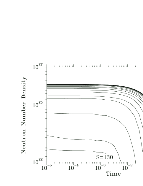
Figure 4: Neutron number density $n_{n}$ as a function of time $t$ for adiabatic expansion with $Y_{e}=0.45$, $\tau_{\rm dyn}\sim 0.05$ s, and $S=130$–350. A superposition of these conditions with approximately equal weights can account for the solar $r$-pattern from the peak at $A=130$ up to the peak at $A=195$. Note that the dynamic timescale $\tau_{\rm dyn}$ used here corresponds to a parametrization of $T(t)$ that is different from Eq. (21). See [21] for details.

Some comments on the use of the solar $r$-pattern in parametric studies are in order. The traditional calculations require that a suitable superposition of the yield patterns resulting from different combinations of $n_{n}$, $T$, and $t_{\rm irr}$ match the solar $r$-pattern shown in Fig. 2 plus a peak at $A=80$. There are several potential problems with this requirement. First, the solar “$r$-process” abundances of the nuclei above the Fe group but with $A\>\lower 1.72218pt\hbox{$\stackrel{{\scriptstyle\scriptstyle<}}{{\scriptstyle\sim}}$}\>90$–110 were derived by subtracting the calculated $s$-process contributions from the total solar abundances [6] and may contain substantial contributions from the $\alpha$-process, which can produce many of these nuclei [24]. Therefore, the results based on fitting the solar “$r$-pattern” associated with the peak at $A=80$ and possibly up to the nuclei with $A\sim 110$ must be viewed with caution. Furthermore, as will be discussed in Sec. 4, the basic templates underlying the overall solar $r$-pattern may be more complicated than those employed in the traditional calculations. The $r$-process yield pattern also depends on the nuclear physical input, almost all of which are calculated from theory with little experimental guidance. In view of the above issues, parametric studies may be of more general use if they are based on the simple criterion that an $r$-process must have an initial neutron-to-seed ratio $R_{n/s}(t_{0})=\langle A\rangle-A_{s}$ in order to produce nuclei with an average mass number $\langle A\rangle$ from the seed nuclei with mass number $A_{s}$. In contrast to the case of the $r$-process, the essential nuclear physical input is known for the $\alpha$-process that determines $R_{n/s}(t_{0})$ and $A_{s}$.

Parametric studies of the $r$-process have the advantage that no specific astrophysical models are required. This also leads to some serious flaws. For example, the parametric studies based on adiabatic expansion cannot give the absolute amount of material that has a specific combination of $Y_{e}$, $S$, and $\tau_{\rm dyn}$. Furthermore, a real $r$-process environment may be improperly characterized by some parametric studies. This flaw has already been demonstrated by the traditional calculations with constant $n_{n}$ and $T$. In addition to the problem with the parameter $t_{\rm irr}$, the freeze-out of the $r$-process is treated as instantaneous in such calculations. However, the actual freeze-out is a multi-stage process during which the $r$-process yield pattern may be smoothed independent of $\beta$-delayed neutron emission (e.g., [21, 27]). It was also proposed [29] that effects during the freeze-out could be responsible for the small peak in the rare earth region ($A\sim 160$) of the solar $r$-pattern (see Fig. 2). Such details of the freeze-out are revealed only when the time evolution of $n_{n}$ and $T$ in the $r$-process event is taken into account. In many respects, the calculations based on adiabatic expansion are more realistic. However, it is quite possible that they still miss some important ingredient. For example, additional parameters characterizing the neutrino fluxes may be required if the $r$-process occurs in core-collapse supernovae (see Sec. 3.1.1).

3 Astrophysical Models of the $r$-Process

A neutron-rich environment is required for an $r$-process. It is interesting to survey the possibilities to obtain such environments during the evolution of the universe. After the big bang, the universe goes through some phase transitions, which might produce density inhomogeneities of such large sizes that only neutrons but not protons can diffuse to uniformity prior to the onset of big bang nucleosynthesis. This segregation of neutrons and protons could result in neutron-rich regions where a primordial $r$-process might occur (e.g., [30, 31]). The details of such a scenario will not be discussed here as its prediction of a minimum $r$-process enrichment lacks observational support. The major outcome of big bang nucleosynthesis is an overall proton-rich nuclear composition with $\approx 76\%$ of H and $\approx 24\%$ of ⁴He by mass. This composition has hardly changed over the history of the universe. Subsequent to big bang nucleosynthesis, neutron excess can be produced locally by processes of weak interaction inside stars. Indeed, the small neutron excess generated by $\beta^{+}$ decay during evolution of stars with masses of $M>10\,M_{\odot}$ is crucial to the production of the solar abundance pattern for the nuclei from ²³Na to the Fe group (e.g., [32]). Weak interaction also participates in the reaction sequence of $p+{{}^{12}{\rm C}}\to{{}^{13}{\rm N}}+\gamma$, ${{}^{13}{\rm N}}\to{{}^{13}{\rm C}}+e^{+}+\nu_{e}$, and $\alpha+{{}^{13}{\rm C}}\to{{}^{16}{\rm O}}+n$, which is the main neutron source for the $s$-process in AGB stars (e.g., [11]). The most dramatic production of neutron excess occurs during the deleptonization of a protoneutron star that is produced by the gravitational collapse of a stellar core. Over a period of $\sim 10$ s, the protoneutron star loses nearly all of its initial electrons and protons through the neutronization reaction $e^{-}+p\to n+\nu_{e}$. Concurrently with the deleptonization, the protoneutron star also releases its enormous gravitational binding energy through emission of $\nu_{e}$, $\bar{\nu}_{e}$, $\nu_{\mu}$, $\bar{\nu}_{\mu}$, $\nu_{\tau}$, and $\bar{\nu}_{\tau}$. The interaction between the neutrinos and the material above the protoneutron star drives a supernova explosion on a timescale of $<1$ s (e.g., [33]) and ejects a small amount of material in a wind that lasts for a period of $\sim 10$ s (e.g., [34]). The neutron-richness of the wind material is set by the competition between the reactions $\nu_{e}+n\to p+e^{-}$ and $\bar{\nu}_{e}+p\to n+e^{+}$ (e.g., [35, 36]). The high neutron number density of $>10^{20}$ cm^-3 required for the $r$-process (see Sec. 2 and Fig. 4) may be obtained in the neutrino-driven wind associated with protoneutron star formation in core-collapse supernovae. Material with such neutron number density may also be ejected when an old neutron star is disrupted during its merging with another neutron star or a black hole. The core-collapse supernova and neutron star merger models of the $r$-process are discussed in detail below.

3.1 Core-collapse supernova models of the $r$-process

The evolution, explosion, and nucleosynthesis of massive stars are a rich subject (see [37] for a recent review). Only a simple sketch of the evolution and explosion of such stars is given here to provide some general astrophysical context for the discussion of the $r$-process. Through various stages of hydrostatic burning, massive stars with $M>10\,M_{\odot}$ develop an onion-skin structure with an Fe core surrounded by shells of successively lighter elements from Si to H. As no more nuclear binding energy can be released by burning Fe, the Fe core undergoes gravitational collapse. When the inner core reaches nuclear density, it becomes a protoneutron star and bounces. This launches a shock, which fails to exit the outer core mainly due to energy loss from dissociation of Fe. Although a successful mechanism remains to be demonstrated (see [38] for a review), it is considered that the shock is revived by the neutrinos emitted from the protoneutron star and proceeds to make a Type II supernova (SN II). Massive stars with $8\,M_{\odot}\>\lower 1.72218pt\hbox{$\stackrel{{\scriptstyle\scriptstyle<}}{{\scriptstyle\sim}}$}\>M\>\lower 1.72218pt\hbox{$\stackrel{{\scriptstyle\scriptstyle<}}{{\scriptstyle\sim}}$}\>10\,M_{\odot}$ develop a degenerate O-Ne-Mg core with insignificant shells [39]. The core collapse in this case is triggered by electron capture [40] and again leads to protoneutron star formation and an SN II [41, 42]. A bare white dwarf in a binary may also collapse into a protoneutron star due to mass accretion from its binary companion [43]. The supernovae resulting from accretion-induced collapse of white dwarfs are sometimes referred to as the “silent supernovae” due to the lack of prominent optical display.

Whether formed by Fe core collapse, O-Ne-Mg core collapse, or accretion-induced collapse (AIC) of a white dwarf, the protoneutron star releases its gravitational binding energy through neutrino emission, the characteristics of which have been modeled by numerical transport calculations (e.g., [44]–[49]). The gravitational binding energy of a protoneutron star with a mass of $M_{\rm NS}\sim 1.4\,M_{\odot}$ and a radius of $R_{\rm NS}\sim 10$ km is $\sim(3/5)GM_{\rm NS}^{2}/R_{\rm NS}\sim 3\times 10^{53}$ erg, where $G$ is the gravitational constant. This energy is emitted approximately equally in each neutrino species over the neutrino diffusion timescale. All neutrino species have neutral-current scattering on nucleons and diffuse out of the protoneutron star on a timescale of $\sim 10$ s. The neutrino luminosities satisfy

$$L_{\nu_{e}}\sim L_{\bar{\nu}_{e}}\sim L_{\nu_{\mu}}\approx L_{\bar{\nu}_{\mu}}\approx L_{\nu_{\tau}}\approx L_{\bar{\nu}_{\tau}}$$ (26)

and have a typical value of $\sim 10^{51}$ erg s^-1 for each species. During diffusion, different neutrino species stop exchanging energy with matter in different decoupling regions, the temperatures of which characterize the neutrino energy spectra emergent from the protoneutron star. Energy exchange with matter occurs mainly through neutral-current scattering on electrons for $\nu_{\mu}$, $\bar{\nu}_{\mu}$, $\nu_{\tau}$, and $\bar{\nu}_{\tau}$, but mainly through the charged-current reactions $\nu_{e}+n\to p+e^{-}$ and $\bar{\nu}_{e}+p\to n+e^{+}$ with higher efficiency for $\nu_{e}$ and $\bar{\nu}_{e}$. In fact, energy exchange is more efficient through $\nu_{e}+n\to p+e^{-}$ than through $\bar{\nu}_{e}+p\to n+e^{+}$ as there are more neutrons than protons inside the protoneutron star. Consequently, the decoupling from local thermodynamic equilibrium with matter occurs first for $\nu_{\mu}$, $\bar{\nu}_{\mu}$, $\nu_{\tau}$, and $\bar{\nu}_{\tau}$, next for $\bar{\nu}_{e}$, and last for $\nu_{e}$. Thus, the average energies corresponding to the emergent neutrino spectra satisfy

$$\langle E_{\nu_{\mu}}\rangle\approx\langle E_{\bar{\nu}_{\mu}}\rangle\approx\langle E_{\nu_{\tau}}\rangle\approx\langle E_{\bar{\nu}_{\tau}}\rangle>\langle E_{\bar{\nu}_{e}}\rangle>\langle E_{\nu_{e}}\rangle$$ (27)

with typical values of $\langle E_{\nu_{e}}\rangle\approx 11$ MeV, $\langle E_{\bar{\nu}_{e}}\rangle\approx 16$ MeV, and $\langle E_{\nu_{\mu}}\rangle\approx 25$ MeV.

Close to the protoneutron star, the temperature is $T\>\lower 1.72218pt\hbox{$\stackrel{{\scriptstyle\scriptstyle>}}{{\scriptstyle\sim}}$}\>10^{10}$ K and the material is in NSE with its nuclear composition dominated by nucleons. This material is heated by the reactions $\nu_{e}+n\to p+e^{-}$ and $\bar{\nu}_{e}+p\to n+e^{+}$ and expands away from the protoneutron star as a neutrino-driven wind. Above a radius corresponding to $T\sim 6\times 10^{9}$ K, the neutrino reactions become inefficient due to the ever-decreasing neutrino flux. The wind material then essentially undergoes adiabatic expansion with fixed values of $Y_{e}$, $S$, and $\tau_{\rm dyn}$ as in the parametric $r$-process study described in Sec. 2. The parameters $Y_{e}$, $S$, and $\tau_{\rm dyn}$ in the wind are determined by the history of neutrino interaction with the wind material at $T\>\lower 1.72218pt\hbox{$\stackrel{{\scriptstyle\scriptstyle>}}{{\scriptstyle\sim}}$}\>10^{10}$ K [36]. In particular, $Y_{e}$ is set at sufficiently low values of $T$ so that the rates $\lambda_{e^{+}n}$ and $\lambda_{e^{-}p}$ for the reactions $e^{+}+n\to p+\bar{\nu}_{e}$ and $e^{-}+p\to n+\nu_{e}$ are unimportant compared with the rates $\lambda_{\nu_{e}n}$ and $\lambda_{\bar{\nu}_{e}p}$ for the reactions $\nu_{e}+n\to p+e^{-}$ and $\bar{\nu}_{e}+p\to n+e^{+}$. This gives an estimate of $Y_{e}$ as [35]

$$Y_{e}\approx{\lambda_{\nu_{e}n}\over\lambda_{\nu_{e}n}+\lambda_{\bar{\nu}_{e}p}}={1\over 1+(\lambda_{\bar{\nu}_{e}p}/\lambda_{\nu_{e}n})}.$$ (28)

With $L_{\nu_{e}}\sim L_{\bar{\nu}_{e}}$ and $\langle E_{\bar{\nu}_{e}}\rangle>\langle E_{\nu_{e}}\rangle$, it was shown that $\lambda_{\bar{\nu}_{e}p}>\lambda_{\nu_{e}n}$, and hence, $Y_{e}<0.5$ can be obtained at least for some part of the period of $\sim 10$ s over which the neutrino-driven wind occurs [36]. This wind was first proposed as a site of the $r$-process in [50]. However, only one SN II model gave the adequate values of $Y_{e}$, $S$, and $\tau_{\rm dyn}$ for producing the peaks at $A=130$ and 195 in the solar $r$-pattern [51]. The typical values of $0.45\>\lower 1.72218pt\hbox{$\stackrel{{\scriptstyle\scriptstyle<}}{{\scriptstyle\sim}}$}\>Y_{e}<0.5$, $S\sim 100$, and $0.01\ {\rm s}\>\lower 1.72218pt\hbox{$\stackrel{{\scriptstyle\scriptstyle<}}{{\scriptstyle\sim}}$}\>\tau_{\rm dyn}\>\lower 1.72218pt\hbox{$\stackrel{{\scriptstyle\scriptstyle<}}{{\scriptstyle\sim}}$}\>0.1$ s obtained in another SN II model [25] and in analytic and numerical studies of the neutrino-driven wind [36, 52] were unable to give an $r$-process (see Fig. 3). Parametric studies of $r$-process nucleosynthesis in the neutrino-driven wind were carried out in [26]–[28].

3.1.1 effects of neutrinos

As will be discussed in Sec. 4.3, in order to account for the solar $r$-process abundances associated with the peaks at $A=130$ and 195, each supernova must eject $\sim 10^{-6}$–$10^{-5}\,M_{\odot}$ of $r$-process material. Although the current neutrino-driven wind models have difficulty in providing the $r$-process conditions, the wind naturally ejects $\sim 10^{-6}$–$10^{-5}\,M_{\odot}$ of material over a period of $\sim 1$ s. This is because the small heating rate due to the weakness of neutrino interaction permits material to escape from the deep gravitational potential of the protoneutron star at a typical rate of $\sim 10^{-6}$–$10^{-5}\,M_{\odot}$ s^-1 [36, 52]. Indeed, the ability to eject a tiny but interesting amount of material was recognized as an attractive feature of the neutrino-driven wind model of the $r$-process (e.g., [26]). On average, a nucleon obtains $\sim 20$ MeV from each interaction with $\nu_{e}$ or $\bar{\nu}_{e}$. In order to escape from the protoneutron star gravitational potential of $GM_{\rm NS}m_{u}/R_{\rm NS}\sim 200$ MeV, a nucleon in the wind must interact with $\nu_{e}$ and $\bar{\nu}_{e}$ for $\sim 10$ times. This suggests that the effects of neutrino interaction may be important even during the essentially adiabatic expansion of the wind material. Some of these effects are discussed below in connection with $r$-process nucleosynthesis.

At $T\>\lower 1.72218pt\hbox{$\stackrel{{\scriptstyle\scriptstyle>}}{{\scriptstyle\sim}}$}\>10^{10}$ K, the evolution of $Y_{e}$ in the wind material is governed by

$$\dot{Y}_{e}=(\lambda_{\nu_{e}n}+\lambda_{e^{+}n})Y_{n}-(\lambda_{\bar{\nu}_{e}p}+\lambda_{e^{-}p})Y_{p}=\lambda_{\nu_{e}n}+\lambda_{e^{+}n}-(\lambda_{\nu_{e}n}+\lambda_{\bar{\nu}_{e}p}+\lambda_{e^{+}n}+\lambda_{e^{-}p})Y_{e},$$ (29)

where $Y_{n}=1-Y_{e}$ and $Y_{p}=Y_{e}$ have been used to obtain the second equality. For small values of $\tau_{\rm dyn}$, $Y_{e}$ freezes out with a value given by Eq. (28) when $T$ is so low that $\lambda_{e^{+}n}$ and $\lambda_{e^{-}p}$ can be neglected compared with $\lambda_{\nu_{e}n}$ and $\lambda_{\bar{\nu}_{e}p}$ but nucleons still dominate the nuclear composition. However, if neutrino interaction continues to be significant when NSE starts to favor $\alpha$-particles over nucleons at $T<10^{10}$ K, the equation governing the evolution of $Y_{e}$ becomes

$$\dot{Y}_{e}\approx\lambda_{\nu_{e}n}+(\lambda_{\bar{\nu}_{e}p}-\lambda_{\nu_{e}n}){X_{\alpha}\over 2}-(\lambda_{\bar{\nu}_{e}p}+\lambda_{\nu_{e}n})Y_{e},$$ (30)

which is obtained by neglecting $\lambda_{e^{+}n}$ and $\lambda_{e^{-}p}$ and using $Y_{n}=1-Y_{e}-(X_{\alpha}/2)$ and $Y_{p}=Y_{e}-(X_{\alpha}/2)$, with $X_{\alpha}$ being the mass fraction of $\alpha$-particles, in the first equality of Eq. (29). In the presence of $\alpha$-particles, the evolution of $Y_{e}$ tries to reach

$$Y_{e}\approx{\lambda_{\nu_{e}n}\over\lambda_{\bar{\nu}_{e}p}+\lambda_{\nu_{e}n}}+{\lambda_{\bar{\nu}_{e}p}-\lambda_{\nu_{e}n}\over\lambda_{\bar{\nu}_{e}p}+\lambda_{\nu_{e}n}}\left({X_{\alpha}\over 2}\right),$$ (31)

which is increased from the value in Eq. (28) for $\lambda_{\bar{\nu}_{e}p}>\lambda_{\nu_{e}n}$. This so-called $\alpha$-effect was first discussed in [53]. Depending on $\tau_{\rm dyn}$, the $\alpha$-effect may significantly decrease the initial neutron-to-seed ratio and hinder the $r$-process [54]. The effects of neutrino interaction with nucleons and nuclei on the evolution of $Y_{e}$ were studied in detail in [55].

For large values of $S$ and $\tau_{\rm dyn}$, the $\alpha$-particles present an additional problem due to their own interaction with neutrinos. In particular, $\nu_{\mu}$, $\bar{\nu}_{\mu}$, $\nu_{\tau}$, and $\bar{\nu}_{\tau}$ with the highest average energy can induce proton spallation on the $\alpha$-particles. The daughter nucleus ³H from this process provides a new path to produce the seed nuclei starting with the reactions $\alpha+{{}^{3}{\rm H}}\to{{}^{7}{\rm Li}}+\gamma$ and $\alpha+{{}^{7}{\rm Li}}\to{{}^{11}{\rm B}}+\gamma$. As this path does not involve the inefficient three-body reactions to burn the $\alpha$-particles (see Sec. 2.2), the production of the seed nuclei can be significantly enhanced, which reduces the initial neutron-to-seed ratio and again hinders the $r$-process [56].

Provided that the above two problems can be avoided and an $r$-process occurs in the neutrino-driven wind, neutrino interaction may have some direct effects on $r$-process nucleosynthesis. First of all, the progenitor nuclei encountered during the $r$-process are extremely neutron-rich and have large cross sections for $\nu_{e}$ capture (see [57, 58] for recent calculations). In contrast to $\beta$ decay, $\nu_{e}$ capture on the progenitor nuclei are insensitive to the presence of magic neutron numbers. Because the abundance peaks at $A=130$ and 195 in the solar $r$-pattern are usually attributed to the slow $\beta$-decay rates of the progenitor nuclei with the magic neutron numbers $N=82$ and 126, respectively, no such peaks would be produced if the rates for $\nu_{e}$ capture were to dominate those for $\beta$ decay at the freeze-out of the $r$-process [53]. However, as the $r$-process proceeds in the wind material, this material is also expanding away from the protoneutron star. Consequently, the neutrino flux, and hence, the neutrino interaction experienced by the wind material decreases during the $r$-process. It is possible that $\nu_{e}$ capture is significant in the early phase of the $r$-process but becomes negligible compared with $\beta$ decay at the freeze-out [59, 60]. In this case, $\nu_{e}$ capture can accelerate the progress from one isotopic chain to the next and reduce the duration of the $r$-process as proposed in [61]. The effects of $\nu_{e}$ capture on the $r$-process flow were also discussed in [62, 63].

Neutrino interaction may also be important during decay towards stability after the $r$-process freezes out. Both $\nu_{e}$ capture and neutral-current reactions with $\nu_{\mu}$, $\bar{\nu}_{\mu}$, $\nu_{\tau}$, and $\bar{\nu}_{\tau}$ can greatly excite the progenitor nuclei, which then deexcite through neutron emission (see [57, 58] for recent calculations) or possibly fission. It was shown that the solar $r$-process abundances of the nuclei with $A=124$–126 and $A=183$–187 may be completely accounted for by neutrino-induced neutron emission from the progenitor nuclei in the abundance peaks at $A=130$ and 195, respectively [59, 64]. This neutrino postprocessing effect is shown for the mass region near $A=195$ in Fig. 5. This effect also constrains the total exposure to neutrinos after the freeze-out as too much neutrino postprocessing overproduces the nuclei below the abundance peaks at $A=130$ and 195 [59, 64]. The effect of neutrino-induced fission during decay towards stability will be discussed in Sec. 4.3.2 in connection with the $r$-patterns observed in metal-poor stars.

Figure 5: Effect of neutrino postprocessing for the mass region near the abundance peak at $A=195$. The abundances before and after the postprocessing are given by the solid and dashed curves, respectively. The filled circles (some with error bars) give the solar $r$-process abundances. The region with $A=183$–187 is highlighted in the inset. See [59, 64] for details.

With a number of possible effects of neutrinos, it is important to do a self-consistent study that includes all the neutrino interaction processes. A significant step in this direction was taken in [54], where a comparison was made between the results calculated by including neutrino interaction to various extent during adiabatic expansion of the wind material. However, this comparison was based on a fixed set of wind parameters and the neutrino luminosities used to calculate the neutrino reaction rates were not compatible with the parameter $\tau_{\rm dyn}$ adopted for the wind. In a fully self-consistent study, the wind parameters such as $S$ and $\tau_{\rm dyn}$ should be determined by the same neutrino emission characteristics that are used to study the neutrino effects on $r$-process nucleosynthesis. It is essential that such a study be carried out in the future.

3.1.2 remedies for the neutrino-driven wind model of the $r$-process

As will be discussed in Sec. 4, a number of observations are in support of core-collapse supernovae being the major site of the $r$-process. The amount of $r$-process material required from each supernova to account for the solar $r$-process abundances associated with the peaks at $A=130$ and 195 is approximately the same as the amount of ejecta in the neutrino-driven wind. However, current models fail to provide the conditions for an $r$-process to occur in the wind. This failure may simply reflect the uncertainties in the models and can be remedied when better physical input is used. A major uncertainty in the wind models concerns the properties of hot and dense matter, which affect the protoneutron star mass $M_{\rm NS}$ and radius $R_{\rm NS}$. General relativistic effects are crucial when $2GM_{\rm NS}/(R_{\rm NS}c^{2})$ ($c$ being the speed of light) approaches unity. For the nominal values of $M_{\rm NS}=1.4\,M_{\odot}$ and $R_{\rm NS}=10$ km, such effects already lead to significantly larger values of $S$ and smaller values of $\tau_{\rm dyn}$ than given by Newtonian calculations for the neutrino-driven wind [36]. Both increase of $S$ and decrease of $\tau_{\rm dyn}$ tend to increase the initial neutron-to-seed ratio for the $r$-process (see Sec. 2.3). Thus, massive and/or compact protoneutron stars with large values of $2GM_{\rm NS}/(R_{\rm NS}c^{2})$ may have a wind with adequate conditions for an $r$-process (see [36, 52] and [65]–[67]). The properties of hot and dense matter also affect neutrino interaction processes in protoneutron stars, and hence, the neutrino emission characteristics obtained from transport calculations (e.g., [68]–[70]). The parameter $Y_{e}$ for the neutrino-driven wind is sensitive to the difference between the rates $\lambda_{\nu_{e}n}$ and $\lambda_{\bar{\nu}_{e}p}$ (see Eq. [28]), which are determined by the emission characteristics of $\nu_{e}$ and $\bar{\nu}_{e}$ [35, 36, 71]. It remains to be seen if low values of $Y_{e}$ favorable for an $r$-process might result from neutrino transport calculations based on better understanding of the properties of hot and dense matter.

Another major uncertainty in the neutrino-driven wind models concerns the properties of neutrinos. As mentioned above, $Y_{e}$ for the wind is sensitive to the difference between the rates $\lambda_{\nu_{e}n}$ and $\lambda_{\bar{\nu}_{e}p}$. Because the average energy of $\nu_{\mu}$, $\bar{\nu}_{\mu}$, $\nu_{\tau}$, and $\bar{\nu}_{\tau}$ is higher than that of either $\nu_{e}$ or $\bar{\nu}_{e}$ [see Eq. (27)], neutrino flavor transformation between the former group and the latter can greatly affect $\lambda_{\nu_{e}n}$ and $\lambda_{\bar{\nu}_{e}p}$, and hence, $Y_{e}$ [35]. There might also exist a sterile neutrino that has no standard weak interaction. Flavor transformation involving the sterile neutrino can dramatically decrease $Y_{e}$ in the neutrino-driven wind by reducing the $\nu_{e}$ flux [72, 73]. With the $\nu_{e}$ flux greatly reduced in the region where $\alpha$-particles are being formed, the $\alpha$-effect is also rendered inoperative [72, 73]. Therefore, sterile neutrinos may play an essential role in enabling $r$-process nucleosynthesis in the neutrino-driven wind. Evidence for the existence of such neutrinos may come from future experiments on neutrino oscillations.

In typical neutrino-driven wind models, various neutrino interaction processes provide the energy for driving the wind. The radial distribution of these energy sources has significant effects on the parameters $S$ and $\tau_{\rm dyn}$ for the wind [36]. A broad distribution above the radius at which the total energy deposition rate peaks tends to favor an $r$-process by increasing $S$ and decreasing $\tau_{\rm dyn}$ [36, 52]. Such a distribution may be obtained when neutrino flavor transformation or especially some extra energy source other than neutrino interaction (e.g., magnetic field and rotation of the neutron star [36]) is included in the wind models.

In considering the neutrino-driven wind model of the $r$-process, it is also important to note the difference between the winds associated with Fe core collapse, O-Ne-Mg core collapse, and AIC of a white dwarf. Although the mass ejection rate and $S$ in the wind are determined near the protoneutron star, the structure of the wind further away may be affected by the outer boundary imposed by the supernova (e.g., [36]). For example, the reverse shock in the Fe-core-collapse events may slow down the wind significantly [36, 52] whereas no such shock is present in the O-Ne-Mg-core-collapse or AIC events. This may have important consequences for $r$-process nucleosynthesis associated with core-collapse supernovae.

3.1.3 other core-collapse supernova models of the $r$-process

The neutrino-driven wind model of the $r$-process is closely related to the neutrino-driven mechanism of core-collapse supernovae. It is recognized that this mechanism crucially depends on neutrino transport and convection (see [38] for a review), a simultaneous and full treatment of which is very difficult to implement numerically. Thus, the robustness of this mechanism remains to be demonstrated. Two alternative explosion mechanisms were proposed for core-collapse supernovae and both have associated $r$-process scenarios. In the prompt mechanism, the bounce of the inner core upon reaching nuclear density launches an energetic shock, which then drives a successful explosion (e.g., [38]). This mechanism might possibly work for the accretion-induced collapse of white dwarfs and the collapse of O-Ne-Mg cores and maybe some low-mass Fe cores. The inner ejecta from a prompt explosion is neutron-rich and has been studied as a possible site of the $r$-process [41, 74, 75]. However, the conditions in this ejecta and the amount of ejected $r$-process material are quite uncertain as the prompt mechanism underlying this $r$-process model is even more problematic than the neutrino-driven mechanism. Another supernova mechanism relies on the formation of magnetohydrodynamic jets following the core collapse (e.g., [76]–[78]). While $r$-process nucleosynthesis associated with jets was discussed quite some time ago [79], an intriguing new scenario was proposed by Cameron [80] recently. In this scenario, jets are associated with the formation of an accretion disk around the protoneutron star. The accretion disk has such high densities that electrons are degenerate but neutrinos can escape. The chemical equilibrium among neutrons, protons, nuclei, and electrons results in large abundance ratios of neutrons to heavy nuclei in the disk. The $r$-process was considered to occur as material is transported from the disk to the base of the jets and ejected. Clearly, more quantitative studies of this $r$-process model are worth pursuing.

3.2 Neutron star merger models of the $r$-process

Two binary neutron star (NS-NS) systems, PSR 1913+16 [81] and PSR 1534+12 [82], were observed in the Galaxy. The neutron stars in an NS-NS binary eventually merge due to orbital decay caused by gravitational radiation. The total time from birth to merger is $\approx 4\times 10^{8}$ yr for PSR 1913+16 and $\approx 3\times 10^{9}$ yr for PSR 1534+12 [83]. Estimates for the rate of NS-NS mergers in the Galaxy range from $\sim 10^{-6}$ to $\sim 3\times 10^{-4}$ yr^-1 with the best guess being $\sim 10^{-5}$ yr^-1 (e.g., [83]–[85]). The birth rates of neutron star-black hole (NS-BH) and NS-NS binaries are comparable. However, the fraction of NS-BH binaries having the appropriate orbital periods for merging within the age of the universe ($\sim 10^{10}$ yr) is uncertain due to their complicated evolution involving mass exchange [83]. In any case, the total rate of neutron star (including NS-NS and NS-BH) mergers in the Galaxy is perhaps $\sim 10^{-5}$ yr^-1, which is $\sim 10^{3}$ times smaller than the Galactic rate of SNe II [86]. This means that each merger must eject $\>\lower 1.72218pt\hbox{$\stackrel{{\scriptstyle\scriptstyle>}}{{\scriptstyle\sim}}$}\>10^{-3}\,M_{\odot}$ of $r$-process material if neutron star mergers were solely responsible for the solar $r$-process abundances associated with the peaks at $A=130$ and 195 ($\sim 10^{-6}$–$10^{-5}\,M_{\odot}$ of $r$-process material is required from each event in the case of core-collapse supernovae).

It was estimated that $\>\lower 1.72218pt\hbox{$\stackrel{{\scriptstyle\scriptstyle<}}{{\scriptstyle\sim}}$}\>5\%$ of the original neutron star mass may be ejected during tidal disruption of the neutron star in an NS-BH merger [87, 88]. Estimates for the amount of cold neutron star matter ejected during an NS-NS merger range from $\sim 10^{-4}\,M_{\odot}$ to $\sim 4\times 10^{-2}\,M_{\odot}$ [89]–[92]. The ejected cold neutron star matter is decompressed and heated to high temperature ($\>\lower 1.72218pt\hbox{$\stackrel{{\scriptstyle\scriptstyle>}}{{\scriptstyle\sim}}$}\>10^{9}$ K) by $\beta$ decay and possibly fission [93, 94]. Further evolution of the decompressed neutron star matter is similar to the adiabatic expansion of neutron-rich matter described in Sec. 2 and could lead to an $r$-process. The $r$-patterns resulting from decompression of cold neutron star matter with $Y_{e}=0.05$, 0.10, 0.12, and 0.15 [94] are shown in Fig. 6. For these values of $Y_{e}$, fission cycling occurs and only the heavy $r$-process nuclei with $A>130$ are produced. Neutron star mergers over the Galactic history would make significant contributions or even completely account for the solar $r$-process abundances at $A>130$ (e.g., [87, 88] and [93]–[95]) if $\sim 10^{-3}\,M_{\odot}$ of cold neutron star matter with $Y_{e}\approx 0.1$ could be ejected from each event. The implications of meteoritic data and stellar observations for this $r$-process model will be discussed in Sec. 4.

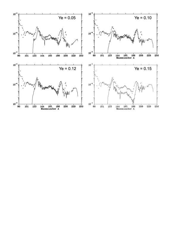
Figure 6: The $r$-patterns (solid curves) resulting from decompression of cold neutron star matter with $Y_{e}=0.05$, 0.10, 0.12, and 0.15, which may be ejected from neutron star mergers. The solar $r$-pattern (pluses) is also shown for comparison. See [94] for details.

Several issues regarding the neutron star merger model of the $r$-process need to be addressed. First of all, numerical calculations gave a wide range for the amount of cold neutron star matter ejected during an NS-NS merger. It was found that this amount sensitively depends on the initial spins of the neutron stars and on the equation of state at high density [90]–[92]. General relativity may also be important. All these issues should be examined by future numerical studies with higher resolutions (a high-resolution Newtonian calculation was recently carried out in [96]). Simulations of an NS-BH merger are also needed to determine the actual amount of ejecta in such events. The other major uncertainty in the neutron star merger model of the $r$-process concerns $Y_{e}$ in the ejecta. The values of $Y_{e}$ not only depend on which part of the neutron star is ejected but may also be affected by weak interaction with $e^{-}$, $e^{+}$, $\nu_{e}$, and $\bar{\nu}_{e}$. Although one study indicated that weak interaction has little effect on $Y_{e}$ and the ejecta essentially retains the $Y_{e}$ values of the cold neutron star matter, such values are still sensitive to the equation of state at high density [92]. In general, as in the case of core-collapse supernovae, much work with improved numerical methods and physical input is required to resolve the outstanding issues regarding neutron star mergers as a possible site of the $r$-process.

3.3 Similarities between core-collapse supernova and neutron star merger models of the $r$-process

Despite many differences between core-collapse supernovae and neutron star mergers, the neutrino-driven wind in the former events and the cold neutron star matter ejected in the latter events follow similar thermodynamic evolution, which may lead to the same generic picture for the $r$-process as described in Sec. 2.3. Furthermore, a neutrino-driven wind can also occur in neutron star mergers [89]. While $\nu_{e}$, $\bar{\nu}_{e}$, $\nu_{\mu}$, $\bar{\nu}_{\mu}$, $\nu_{\tau}$, and $\bar{\nu}_{\tau}$ emitted during such events have approximately the same energy spectra as in the case of core-collapse supernovae, the luminosity of $\bar{\nu}_{e}$ is $\sim 3$ times larger than that of $\nu_{e}$ due to the dominant production of $\bar{\nu}_{e}$ via the reaction $e^{+}+n\to p+\bar{\nu}_{e}$ [89, 92]. Consequently, the neutrino-driven wind from neutron star mergers can have $Y_{e}$ values much less than 0.5 [see Eq. (28)]. It was estimated that $\sim 10^{-4}$–$10^{-2}\,M_{\odot}$ of very neutron-rich material may be ejected in this wind [89]. However, detailed studies of this wind require much better treatment of neutrino transport than implemented in the existing models [92]. It is important that such studies be carried out in the future.

4 Observational Studies of the $r$-Process

Enormous progress has been made in observational studies of the $r$-process since the last major review by Cowan et al. [9] in 1991. This includes meteoritic evidence for the diversity of $r$-process sources and demonstration of some regularity in $r$-patterns and of large dispersions in $r$-process abundances at low metallicities by observations of metal-poor stars. These observational advances and their implications for the $r$-process are discussed in connection with a three-component model for abundances in metal-poor stars. Other models addressing the abundances in metal-poor stars and their implications for the $r$-process are also described.

4.1 Meteoritic data and diverse sources for the $r$-process

Meteorites were formed during the birth of the solar system $\approx 4.6\times 10^{9}$ yr ago. They provide important information on the inventory of radioactive nuclei in the early solar system (ESS). For example, ¹⁸²Hf has a lifetime of $\tau_{182}=1.3\times 10^{7}$ yr and $\beta$-decays to ¹⁸²Ta, which in turn $\beta$-decays with a lifetime of 165 days to the stable nucleus ¹⁸²W. Any ¹⁸²Hf that had been incorporated into the meteorites decayed to ¹⁸²W long ago. Unlike ¹⁸²W, the stable nuclei ¹⁸⁰Hf and ¹⁸⁴W do not receive any contributions from radioactive decay. As ¹⁸²Hf and ¹⁸⁰Hf are chemically identical, a meteorite with a high abundance of ¹⁸⁰Hf also has a high initial abundance of ¹⁸²Hf. Therefore, if a significant inventory of ¹⁸²Hf existed in the ESS, there would be a linear correlation between the present abundance ratios ¹⁸²W/¹⁸⁴W and ¹⁸⁰Hf/¹⁸⁴W in the meteorites. Such a correlation was found and gave (¹⁸²Hf/¹⁸⁰Hf)${}_{\rm ESS}\approx 10^{-4}$ for the abundance ratio of ¹⁸²Hf to ¹⁸⁰Hf in the ESS [97, 98] (see also [99]–[102]). Similarly, meteoritic measurements gave (¹²⁹I/¹²⁷I)${}_{\rm ESS}\approx 10^{-4}$ for the abundance ratio of ¹²⁹I (with a lifetime of $\tau_{129}=2.3\times 10^{7}$ yr) to ¹²⁷I (stable) in the ESS [103, 104].

The nucleus ¹⁸¹Hf $\beta$-decays with a lifetime of 61 days in the laboratory and cannot provide a significant branching for neutron capture to produce ¹⁸²Hf during the $s$-process. So major production of ¹⁸²Hf can only occur in the $r$-process. Both ¹²⁹I and ¹²⁷I are essentially pure $r$-process nuclei. The meteoritic data on ¹⁸²Hf and ¹²⁹I could not be explained if there were only a unique $r$-process source with a universal yield pattern. This can be shown by the method of contradiction. If ¹⁸²Hf and ¹²⁹I were produced with a yield ratio of $Y_{129}/Y_{182}$ by a unique $r$-process source, then

$$\left({{}^{129}{\rm I}\over{}^{182}{\rm Hf}}\right)_{\rm ESS}>{Y_{129}\over Y_{182}}.$$ (32)

This is because ¹²⁹I survives longer than ¹⁸²Hf. The yield ratio $Y_{129}/Y_{182}$ can be rewritten as

$${Y_{129}\over Y_{182}}={Y_{129}\over Y_{127}}\left({{}^{127}{\rm I}\over{}^{182}{\rm W}_{r}}\right)_{\odot},$$ (33)

where the yield ratio $Y_{127}/Y_{182}$ has been set to be the same as the solar $r$-process abundance ratio of ¹²⁷I to ¹⁸²W (with ¹⁸²W_r being the part of ¹⁸²W contributed by the $r$-process) under the assumption of a universal $r$-process yield pattern. Equations (32) and (33) can be rearranged into

$${(^{129}{\rm I}/^{127}{\rm I})_{\rm ESS}\over(^{182}{\rm Hf}/^{180}{\rm Hf})_{\rm ESS}}>{Y_{129}\over Y_{127}}\left({{}^{180}{\rm Hf}\over{}^{182}{\rm W}_{r}}\right)_{\odot}.$$ (34)

The left-hand side of Eq. (34) is $\approx 1$ based on the meteoritic data, while the right-hand side is $\approx 4$ by taking $Y_{129}/Y_{127}=1.4$ and $(^{180}{\rm Hf}/^{182}{\rm W}_{r})_{\odot}=0.0541/0.019$ [4, 10]. Thus, Eq. (34) is violated by a factor of $\approx 4$ and the underlying assumption that ¹⁸²Hf and ¹²⁹I were produced by a unique $r$-process source must be invalid.

While the diversity of $r$-process sources can be established by using only the meteoritic data on ¹⁸²Hf and ¹²⁹I, more may be learned about the nature of these sources by making the following assumption. Suppose that ¹⁸²Hf and ¹²⁹I are produced by two distinct kinds of $r$-process events, which occurred at regular intervals of $\Delta_{\rm Hf}$ and $\Delta_{\rm I}$, respectively, over a uniform production period of $T_{\rm UP}\approx 10^{10}$ yr prior to the formation of the solar system. If the interval between the last event of each kind and the formation of the solar system is exactly $\Delta_{\rm Hf}$ or $\Delta_{\rm I}$, then

$$\left({{}^{182}{\rm Hf}\over{}^{182}{\rm W}_{r}}\right)_{\rm ESS} = \left({\tau_{182}\over T_{\rm UP}}\right){\Delta_{\rm Hf}/\tau_{182}\over\exp(\Delta_{\rm Hf}/\tau_{182})-1},$$ (35)

$$\left({{}^{129}{\rm I}\over{}^{127}{\rm I}}\right)_{\rm ESS} = \left({Y_{129}\over Y_{127}}\right)\left({\tau_{129}\over T_{\rm UP}}\right){\Delta_{\rm I}/\tau_{129}\over\exp(\Delta_{\rm I}/\tau_{129})-1}.$$ (36)

Equations (35) and (36) are valid for $\Delta_{\rm Hf},\ \Delta_{\rm I}\ll T_{\rm UP}$, in which case the radioactive nuclei in the ESS were contributed by the last few events prior to the formation of the solar system while the stable nuclei were accumulated over essentially the entire period of $T_{\rm UP}$. With $(^{182}{\rm Hf}/^{182}{\rm W}_{r})_{\rm ESS}=(^{182}{\rm Hf}/^{180}{\rm Hf})_{\rm ESS}(^{180}{\rm Hf}/^{182}{\rm W}_{r})_{\odot}=2.8\times 10^{-4}$ and $Y_{129}/Y_{127}=1.4$, Eqs. (35) and (36) can be solved to give $\Delta_{\rm Hf}=3.3\times 10^{7}$ yr and $\Delta_{\rm I}=1.2\times 10^{8}$ yr, which should indeed represent two distinct kinds of $r$-process events. Based on similar arguments, Wasserburg et al. [105] first pointed out that the meteoritic data on ¹⁸²Hf and ¹²⁹I require diverse sources for the $r$-process (see also [106]). In general, other nuclei with $A>130$ are produced together with ¹⁸²Hf while those with $A\>\lower 1.72218pt\hbox{$\stackrel{{\scriptstyle\scriptstyle<}}{{\scriptstyle\sim}}$}\>130$ are produced together with ¹²⁹I. The meteoritic data on ¹⁸²Hf and ¹²⁹I suggest that there must be at least two distinct kinds of $r$-process events: the high-frequency $H$ events producing mainly the heavy $r$-process nuclei with $A>130$ ($H$ stands for “high-frequency” and “heavy $r$-process nuclei”) and the low-frequency $L$ events producing dominantly the light $r$-process nuclei with $A\>\lower 1.72218pt\hbox{$\stackrel{{\scriptstyle\scriptstyle<}}{{\scriptstyle\sim}}$}\>130$ ($L$ stands for “low-frequency” and “light $r$-process nuclei”) [60, 105, 106]. An average interstellar medium (ISM) is enriched with the appropriate $r$-process nuclei at a frequency of $f_{H}=\Delta_{\rm Hf}^{-1}\sim(3\times 10^{7}\ {\rm yr})^{-1}$ by the $H$ events and at a frequency of $f_{L}=\Delta_{\rm I}^{-1}\sim(10^{8}\ {\rm yr})^{-1}$ by the $L$ events.

The frequencies of the $H$ and $L$ events can be compared with the frequencies for replenishment of newly-synthesized material in the ISM by core-collapse supernovae and neutron star mergers. The total kinetic energy of the ejecta from a supernova or neutron star merger is typically $\sim 10^{51}$ erg. The amount of ISM required to dissipate the energy and the momentum of the ejecta is $M_{\rm mix}\sim 3\times 10^{4}\,M_{\odot}$ (e.g., [107]). For a present event rate of $f_{\rm G}$ in the Galaxy corresponding to a total gas mass of $M_{\rm gas}\sim 10^{10}\,M_{\odot}$, the frequency for replenishment of newly-synthesized material in the ISM by the relevant events is

$$f_{\rm mix}=(10^{7}\ {\rm yr})^{-1}\left[{f_{\rm G}\over(30\ {\rm yr})^{-1}}\right]\left({M_{\rm mix}\over 3\times 10^{4}\,M_{\odot}}\right)\left({10^{10}\,M_{\odot}\over M_{\rm gas}}\right).$$ (37)

The present Galactic rate of $\sim(30\ {\rm yr})^{-1}$ for core-collapse supernovae [86] corresponds to $f_{\rm mix}^{\rm SN}\sim(10^{7}\ {\rm yr})^{-1}$ while that of $\sim(10^{5}\ {\rm yr})^{-1}$ for neutron star mergers (e.g., [83]) corresponds to $f_{\rm mix}^{\rm NSM}\sim(3\times 10^{10}\ {\rm yr})^{-1}$. As $f_{H}>f_{L}\gg f_{\rm mix}^{\rm NSM}$, it seems that neutron star mergers cannot be associated with either the $H$ or $L$ events. This conclusion is unaffected if the upper limit of $\sim(10^{4}\ {\rm yr})^{-1}$ [84] instead of the nominal value of $\sim(10^{5}\ {\rm yr})^{-1}$ is used for the present Galactic rate of neutron star mergers. By contrast, $f_{\rm mix}^{\rm SN}$ is comparable to $f_{H}$ and $f_{L}$ within a factor of $\sim 10$, which suggests that the $H$ and $L$ events may be associated with core-collapse supernovae [105, 108]. It is important that the above argument be substantiated by more detailed studies on the mixing of the ejecta from core-collapse supernovae and neutron star mergers with the ISM and on the occurrences of these events over the Galactic history. Independent of the association with specific astrophysical sites, the characteristics of the $H$ and $L$ events are further tested and elucidated by observations of abundances in metal-poor stars.

4.2 Observations of abundances in metal-poor stars

The effects of diverse sources for the $r$-process would be most prominent in the early Galaxy where not many $r$-process events had contributed to the abundances in a reference ISM. The chemical evolution of the early Galaxy is reflected by the abundances in metal-poor stars that reside in the Galactic halo. Observations of abundances in a large number of metal-poor stars as well as detailed studies covering many elements in individual stars have been carried out by a number of groups (e.g., [109]–[119]). These observations provide strong support for the diversity of $r$-process sources and give important information on the $r$-patterns produced by these sources.

Except for the trivial case where an element has a single $r$-process isotope and some special cases [120]–[122] where the hyperfine structure of the atomic spectra allows the extraction of the isotopic composition (see discussion of Ba in Sec. 4.3.2), stellar observations can only give the total abundance of all the isotopes of an element. The observed abundance of an element E in a star is usually given in terms of

$$\log\epsilon({\rm E})=\log({\rm E/H})+12,$$ (38)

where (E/H) is the abundance ratio of the element E relative to hydrogen in the star. Hydrogen is an excellent reference element as its overall abundance has changed little over the history of the universe. The “metallicity” of a star is measured by

$$[{\rm Fe/H}]=\log\epsilon({\rm Fe})-\log\epsilon_{\odot}({\rm Fe})=\log({\rm Fe/H})-\log({\rm Fe/H})_{\odot},$$ (39)

where the subscript “$\odot$” denotes quantities for the sun. There are two possible sources for Fe: SNe II and Ia. However, as SNe Ia are associated with low-mass progenitors that evolve on timescales of $\sim 10^{9}$ yr, only SNe II with short-lived massive progenitors contributed Fe during the first $\sim 10^{9}$ yr subsequent to the onset of Galactic chemical evolution ($t=0$). Over a period of $\sim 10^{10}$ yr prior to the formation of the solar system, SNe II contributed $\sim 1/3$ of the solar Fe abundance (e.g., [123]). This gives

$$\left({{\rm Fe}\over{\rm H}}\right)\sim{1\over 3}\left({{\rm Fe}\over{\rm H}}\right)_{\odot}\left({t\over 10^{10}\ {\rm yr}}\right)$$ (40)

for $t\>\lower 1.72218pt\hbox{$\stackrel{{\scriptstyle\scriptstyle<}}{{\scriptstyle\sim}}$}\>10^{9}$ yr. Thus, for stars with [Fe/H] $\>\lower 1.72218pt\hbox{$\stackrel{{\scriptstyle\scriptstyle<}}{{\scriptstyle\sim}}$}\>-1.5$ corresponding to $t\>\lower 1.72218pt\hbox{$\stackrel{{\scriptstyle\scriptstyle<}}{{\scriptstyle\sim}}$}\>10^{9}$ yr, their Fe abundances are dominated by SN II contributions. Stars with $-3\>\lower 1.72218pt\hbox{$\stackrel{{\scriptstyle\scriptstyle<}}{{\scriptstyle\sim}}$}\>[{\rm Fe/H}]<-2.5$ are referred to as ultra-metal-poor (UMP) stars and those with $-2.5\>\lower 1.72218pt\hbox{$\stackrel{{\scriptstyle\scriptstyle<}}{{\scriptstyle\sim}}$}\>[{\rm Fe/H}]\>\lower 1.72218pt\hbox{$\stackrel{{\scriptstyle\scriptstyle<}}{{\scriptstyle\sim}}$}\>-1.5$ as metal-poor (MP) stars.

The observational data of interest here concern the elements Sr and above. In general, both the $r$-process and the main $s$-process can produce these elements. However, the main $s$-process contributions dominantly come from low-mass AGB stars that evolve on timescales of $\sim 10^{9}$ yr. So the abundances of the elements Sr and above in UMP and MP stars represent the $r$-process contributions as pointed out by Truran [124]. The occurrence of $r$-process events in the early Galaxy ($t\>\lower 1.72218pt\hbox{$\stackrel{{\scriptstyle\scriptstyle<}}{{\scriptstyle\sim}}$}\>10^{9}$ yr) suggests that these events are associated with objects such as SNe II, which have short-lived massive progenitors.

4.2.1 nonsolar $r$-patterns in UMP stars

The observed abundances of a large number of elements in the UMP star CS 22892–052 [110, 114] are shown in Fig. 7. The solar $r$-pattern [10] translated to pass through the Eu data is also shown for comparison. It can be seen that the data on the heavy $r$-process elements from Ba to Ir are in excellent agreement with the translated solar $r$-pattern. However, there are large differences between the data and this pattern in the region of the light $r$-process elements below Ba. It is important to examine how the uncertainties in the solar $r$-process abundances may affect the above comparison. The fraction of the solar abundance contributed by the $s$-process is very small ($\beta_{\odot,s}\>\lower 1.72218pt\hbox{$\stackrel{{\scriptstyle\scriptstyle<}}{{\scriptstyle\sim}}$}\>0.3$) for the following groups of elements: (1) Ru, Rh, and Ag; (2) from Sm to Yb; and (3) Os and Ir [10] (see Table 1 in Sec. 4.2.2). The solar $r$-process abundances of these elements should be rather reliable. Thus, in comparing the data for CS 22892–052 and the translated solar $r$-pattern, the agreement for the elements above Ba in groups (2) and (3) and the disagreement for Rh and Ag below Ba in group (1) are robust. Regardless of the possible uncertainties in the solar $r$-process abundances of the other elements (see discussion of Sr, Y, Zr, Nb, and Ba in Sec. 4.2.2), the observed $r$-pattern in CS 22892–052 is clearly different from the overall solar $r$-pattern. Similar difference is also observed for another UMP star CS 31082–001 [117]. These observations provide strong support for the diversity of $r$-process sources as concluded from the meteoritic data on ¹⁸²Hf and ¹²⁹I. The observed deficiency especially at the light $r$-process elements Rh and Ag relative to the solar $r$-pattern that is translated to pass through the Eu data reflects the characteristics of the $H$ events that produce mainly the heavy $r$-process nuclei. By inference, a mixture of the $H$ events and the $L$ events that produce dominantly the light $r$-process nuclei is then required to account for the overall solar $r$-pattern.

Figure 7: The observed abundances in CS 22892–052 (filled circles with error bars: [110, 114]) compared with the solar $r$-pattern (solid curve: [10]) that is translated to pass through the Eu data. The data on the heavy $r$-process elements from Ba to Ir are in excellent agreement with the translated solar $r$-pattern. However, the data on the light $r$-process elements Rh and Ag clearly fall below this pattern. See text for details. See also Sec. 4.2.2 for discussion of corrections to the solar $r$-process abundances of Sr, Y, Zr, Nb, and Ba.

4.2.2 yields of $H$ and $L$ events and three-component model for abundances in UMP and MP stars

The differences in the observed $r$-process abundances between the UMP stars HD 115444 [113], CS 31082–001 [117], and CS 22892–052 [110, 114] are shown as $\Delta\log\epsilon(Z)=\log\epsilon_{\rm HD115444}(Z)-\log\epsilon_{\rm CS22892}(Z)$ or $\log\epsilon_{\rm CS31082}(Z)-\log\epsilon_{\rm CS22892}(Z)$ in Fig. 8. It can be seen that within the observational uncertainties, these differences represent a uniform shift in $\log\epsilon(Z)$ of $\approx-0.6$ dex for HD 115444 and of $\approx 0.21$ dex for CS 31082–001, both relative to CS 22892–052. This means that these three UMP stars have essentially the same $r$-pattern. This pattern is deficient in the light $r$-process elements such as Rh and Ag relative to the solar $r$-pattern translated to pass through the Eu data (an established result for CS 22892–052, a confirmed prediction for CS 31082–001 [117, 125], and still a prediction for HD 115444), and therefore, is characteristic of the $H$ events (see Sec. 4.2.1). The $H$ events then have an approximately fixed yield pattern, which can be taken from the data for e.g., CS 22892–052. As the $H$ yield pattern coincides with the solar $r$-pattern and the $r$-patterns in a number of MP stars [112, 116] in the region of the heavy $r$-process elements, it is reasonable to assume that these elements are produced exclusively by the $H$ events. In this case, the occurrence of these events can be represented by the abundance of a typical heavy $r$-process element such as Eu.

Figure 8: Differences in the observed $r$-process abundances between HD 115444 [113] and CS 22892–052 [110, 114] (open squares with error bars) and those between CS 31082–001 [117] and CS 22892–052 (filled circles with error bars). The data are consistent with a uniform shift in $\log\epsilon(Z)$ of $\approx-0.6$ dex (lower dashed line) for HD 115444 and of $\approx 0.21$ dex (upper dashed line) for CS 31082–001, both relative to CS 22892–052. This suggests an approximately fixed yield pattern for the $H$ events. The upward offset from the lower dashed line for the elements Sr, Y, and Zr in HD 115444 indicates that this star may have received large contributions to these elements from the $P$ inventory [to be discussed in the text after Eq. (42)] in addition to the $H$ events. By contrast, the abundances of Sr, Y, and Zr in CS 31082–001 and CS 22892–052 are dominated by the contributions from the $H$ events.

Over the period of $T_{\rm UP}\sim 10^{10}$ yr prior to the formation of the solar system, a total number $n_{H}^{\odot}=f_{H}T_{\rm UP}\sim 10^{3}$ of $H$ events contributed to the solar $r$-process abundance of Eu for $f_{H}\sim(10^{7}\ {\rm yr})^{-1}$. This gives (Eu/H)${}_{\odot,r}=n_{H}^{\odot}({\rm Eu/H})_{H}$, or

$$\log\epsilon_{H}({\rm Eu})=\log\epsilon_{\odot,r}({\rm Eu})-\log n_{H}^{\odot}\sim-2.5,$$ (41)

where $\log\epsilon_{\odot,r}({\rm Eu})=0.52$ corresponds to the solar $r$-process abundance of Eu [10] and $\log\epsilon_{H}({\rm Eu})$ represents the Eu abundance resulting from a single $H$ event. The data on Eu over the wide range of $-3\>\lower 1.72218pt\hbox{$\stackrel{{\scriptstyle\scriptstyle<}}{{\scriptstyle\sim}}$}\>[{\rm Fe/H}]\>\lower 1.72218pt\hbox{$\stackrel{{\scriptstyle\scriptstyle<}}{{\scriptstyle\sim}}$}\>-1$ are shown in Fig. 9. The lowest observed Eu abundances are consistent with the enrichment level of $\log\epsilon_{H}({\rm Eu})\sim-2.5$ for a single $H$ event. This consistency further establishes that the frequency of the $H$ events is $f_{H}\sim(10^{7}\ {\rm yr})^{-1}$, which is close to the frequency for replenishing newly-synthesized material in the ISM by core-collapse supernovae (see Sec. 4.1). If $f_{H}$ were $\sim(10^{10}\ {\rm yr})^{-1}$, which is close to the frequency for replenishing newly-synthesized material in the ISM by neutron star mergers (see Sec. 4.1), $n_{H}^{\odot}$ would be $\sim 1$. The corresponding enrichment level of $\log\epsilon_{H}({\rm Eu})\sim 0.52$ for a single $H$ event [see Eq. (41)] would be in clear conflict with the Eu data shown in Fig. 9. This again suggests that the $H$ events cannot be associated with neutron star mergers [108]. A similar argument against the association of the $L$ events with neutron star mergers [108] can be made by using the data on the light $r$-process element Ag [126]. It is important that these arguments be verified by more sophisticated studies on the inhomogeneous chemical evolution of the early Galaxy.

Figure 9: Data on Eu over the wide range of $-3\>\lower 1.72218pt\hbox{$\stackrel{{\scriptstyle\scriptstyle<}}{{\scriptstyle\sim}}$}\>[{\rm Fe/H}]\>\lower 1.72218pt\hbox{$\stackrel{{\scriptstyle\scriptstyle<}}{{\scriptstyle\sim}}$}\>-1$ (filled circles: [115]; open squares: [109]; asterisks: [113]; filled diamond: [114]; filled triangle: [117]). There is a large dispersion of $\sim 2$ dex in $\log\epsilon({\rm Eu})$ at $-3\>\lower 1.72218pt\hbox{$\stackrel{{\scriptstyle\scriptstyle<}}{{\scriptstyle\sim}}$}\>[{\rm Fe/H}]<-2.5$, which suggests that the $H$ events responsible for Eu enrichment cannot produce any significant amount of Fe. The Eu abundance resulting from a single $H$ event (horizontal dashed line) is consistent with the lowest observed Eu abundances. The vertical dashed line indicates the Fe abundance resulting from a single $L$ event. See text for details.

Figure 9 shows that there is a large dispersion of $\sim 2$ dex in $\log\epsilon({\rm Eu})$ over the narrow range of $-3\>\lower 1.72218pt\hbox{$\stackrel{{\scriptstyle\scriptstyle<}}{{\scriptstyle\sim}}$}\>[{\rm Fe/H}]<-2.5$. In particular, CS 31082–001 and CS 22892–052 with the highest Eu abundances among the UMP stars shown in this figure have very low values of [Fe/H] $=-2.9$ and $-3.1$, respectively. This suggests that the $H$ events responsible for Eu enrichment cannot produce any significant amount of Fe [127]. No Fe is expected to be produced in neutron star mergers. However, as argued above, the rarity of these events appears to result in conflicts with both the meteoritic data on ¹⁸²Hf and observations of abundances in metal-poor stars if they are associated with the $H$ events. While the possibility of neutron star mergers being an $r$-process source merits further studies, the discussion below assumes that the $H$ and $L$ events are associated with core-collapse supernovae, which include SNe II from the collapse of O-Ne-Mg and Fe cores as well as the silent supernovae from accretion-induced collapse of white dwarfs. A number of SNe II including SN 1987A are known to produce Fe (see e.g., Table 1 of [128]). In fact, $\sim 1/3$ of the solar Fe abundance is attributed to SNe II (e.g., [123]). As no Fe can be produced by the $H$ events, this Fe must be assigned to a total number $n_{L}^{\odot}=f_{L}T_{\rm UP}\sim 10^{2}$ of $L$ events that occurred with a frequency of $f_{L}\sim(10^{8}\ {\rm yr})^{-1}$ over the period of $T_{\rm UP}\sim 10^{10}$ yr prior to the formation of the solar system. This gives $(1/3){\rm(Fe/H)}_{\odot}\sim n_{L}^{\odot}{\rm(Fe/H)}_{L}$, or

$${\rm[Fe/H]}_{L}\sim-\log(3n_{L}^{\odot})\sim-2.5,$$ (42)

where [Fe/H]_L represents the Fe abundance resulting from a single $L$ event.

The UMP stars have $-3\>\lower 1.72218pt\hbox{$\stackrel{{\scriptstyle\scriptstyle<}}{{\scriptstyle\sim}}$}\>[{\rm Fe/H}]<-2.5$, and therefore, cannot have received any contributions from the $L$ events. The Fe in these stars is attributed to the very massive ($\>\lower 1.72218pt\hbox{$\stackrel{{\scriptstyle\scriptstyle>}}{{\scriptstyle\sim}}$}\>100\,M_{\odot}$) stars that dominated the chemical evolution of the universe until [Fe/H] $\sim-3$ was reached [127]. At this critical metallicity, very massive stars could not be formed any more and major formation of regular ($\sim 1$–$60\,M_{\odot}$) stars took over. In addition to Fe, other elements were also produced by the very massive stars. The inventory of such elements associated with the production of [Fe/H] $\sim-3$ is referred to as the prompt ($P$) inventory. The abundance of an element E in a UMP star represents the sum of the $P$ inventory and the contributions from the $H$ events:

$${\rm(E/H)}={\rm(E/H)}_{P}+{\rm(E/Eu)}_{H}{\rm(Eu/H)},$$ (43)

where (E/H)_P is the $P$ inventory of E and (E/Eu)_H is the relative $H$ yield of E to Eu. The parameter (E/Eu)_H is assumed to be the same for all $H$ events (see Fig. 8). Then the parameters (E/H)_P and (E/Eu)_H can be obtained from the data for two UMP stars with essentially the same [Fe/H] but very different Eu abundances (e.g., CS 22892–052 and HD 115444). It was found that there is a significant $P$ inventory for the light $r$-process elements Sr, Y, and Zr [129]. The parameters (E/H)_P and (E/Eu)_H for these elements are given in terms of $\log\epsilon_{P}({\rm E})$ and $\log\epsilon_{H}({\rm E})$ in Table 1. The parameter (E/Eu)_H can be calculated as

$$\left({{\rm E}\over{\rm Eu}}\right)_{H}=10^{\log\epsilon_{H}({\rm E})-\log\epsilon_{H}({\rm Eu})},$$ (44)

where $\log\epsilon_{H}({\rm E})$ represents the abundance of E resulting from a single $H$ event (the $H$ yield of E) and $\log\epsilon_{H}({\rm Eu})=-2.48$ corresponds to assigning the solar $r$-process abundance of Eu to $n_{H}^{\odot}=10^{3}$ $H$ events [see Eq. (41)]. By assuming that the $P$ inventory is negligible for the elements above Zr, the $\log\epsilon_{H}$ values for the elements from Nb to Cd can be calculated from the data for CS 22892–052. As the heavy $r$-process elements Ba and above follow the solar $r$-pattern, the $\log\epsilon_{H}$ values for these elements can be calculated from the data for CS 22892–052 or from the solar $r$-process abundances as in the case of Eu [see Eq. (41)]. The $\log\epsilon_{H}$ values for the elements above Zr are also given in Table 1. By applying Eq. (43) to the data for UMP stars, it was further found that the $H$ events cannot produce any significant amount of the elements from Na to Ni, which include not only the Fe group but also the so-called “$\alpha$-elements” such as Mg, Si, Ca, and Ti [130].

Table 1: Parameters of the three-component model for abundances in UMP and MP stars (see Table 3 of [129]). The $P$ inventory in col. (2) and the $H$ yields in col. (3) are calculated from the data on HD 115444 [113] and CS 22892–052 [114] for Sr, Y, and Zr. The $P$ inventory for the elements above Zr is assumed to be negligible and set to $-\infty$. The $H$ yields of Nb to Cd are calculated from the data for CS 22892–052 and those of Ba to Au from the standard solar $r$-process abundances [10] in col. (5) [corresponding to the solar $s$-process fractions in col. (6)]. The $L$ yields in col. (4) are calculated from cols. (2), (3), and (5) for Sr to Cd and set to $-\infty$ for Ba and above. The corrected values for Sr, Y, Zr, and Ba are given in cols. (7)–(9). These columns are omitted for La to Au, for which elements no corrections are recommended.

E	$\log\epsilon_{P}({\rm E})$	$\log\epsilon_{H}({\rm E})$	$\log\epsilon_{L}({\rm E})$	$\log\epsilon_{\odot,r}({\rm E})$	$\beta_{\odot,s}({\rm E})$	$\log\epsilon_{L}^{\rm corr}({\rm E})$	$\log\epsilon_{\odot,r}^{\rm corr}({\rm E})$	$\beta_{\odot,s}^{\rm corr}({\rm E})$
(1)	(2)	(3)	(4)	(5)	(6)	(7)	(8)	(9)
Fe	4.51a	$-\infty$	5.03a	—	—	—	—	—
Sr	0.13	$-1.30$	$-\infty^{\rm b}$	1.64	0.95	0.35	2.44	0.69
Y	$-1.05$	$-2.05$	$-1.36$	1.12	0.92	$-0.42$	1.67	0.72
Zr	$-0.13$	$-1.53$	$-0.40$	1.85	0.83	0.26	2.32	0.49
Nb	$-\infty$	$-2.56$	$-2.06$	0.56	0.85	—c	—c	—c
Ru	$-\infty$	$-1.56$	$-0.92$	1.60	0.32	—	—	—
Rh	$-\infty$	$-2.36$	$-1.20$	1.03	0.14	—	—	—
Pd	$-\infty$	$-1.82$	$-0.95$	1.42	0.46	—	—	—
Ag	$-\infty$	$-2.36$	$-1.02$	1.14	0.20	—	—	—
Cd	$-\infty$	$-1.91$	$-0.85$	1.42	0.52	—	—	—
Ba	$-\infty$	$-1.52^{\rm d}$	$-\infty$	1.48	0.81	$-0.47$	1.79	0.62

^a With $\log\epsilon_{\odot}({\rm Fe})=7.51$ [4], these values correspond to [Fe/H]${}_{P}=-3$ and [Fe/H]${}_{L}=-2.48$.
^b The standard solar $r$-process abundance of Sr is saturated by the contributions from $n_{H}^{\odot}=10^{3}$ $H$ events, and therefore, does not allow any contributions to Sr from the $L$ events.
^c The data for BD +17^∘3248 [118] suggest $\log\epsilon_{L}^{\rm corr}({\rm Nb})\approx-0.88$ to $-0.66$, which corresponds to $\log\epsilon_{\odot,r}^{\rm corr}({\rm Nb})\approx 1.20$ to $1.39$ and $\beta_{\odot,s}({\rm Nb})\approx 0.37$ to 0.02. This corrected $L$ yield of Nb should be tested by future data for MP stars.
^d This $H$ yield of Ba, which is calculated by attributing its standard solar $r$-process abundance to $n_{H}^{\odot}=10^{3}$ $H$ events, essentially coincides with the value of $\log\epsilon_{H}({\rm Ba})\approx-1.57$ obtained from the data for CS 22892–052. The use of the latter value is recommended.

Table 1 (continued)

E	$\log\epsilon_{P}({\rm E})$	$\log\epsilon_{H}({\rm E})$	$\log\epsilon_{L}({\rm E})$	$\log\epsilon_{\odot,r}({\rm E})$	$\beta_{\odot,s}({\rm E})$
(1)	(2)	(3)	(4)	(5)	(6)
La	$-\infty$	$-2.22$	$-\infty$	0.78	0.62
Ce	$-\infty$	$-2.02$	$-\infty$	0.98	0.77
Pr	$-\infty$	$-2.51$	$-\infty$	0.49	0.49
Nd	$-\infty$	$-1.90$	$-\infty$	1.10	0.56
Sm	$-\infty$	$-2.20$	$-\infty$	0.80	0.29
Eu	$-\infty$	$-2.48$	$-\infty$	0.52	0.06
Gd	$-\infty$	$-2.00$	$-\infty$	1.00	0.15
Tb	$-\infty$	$-2.70$	$-\infty$	0.30	0.07
Dy	$-\infty$	$-1.92$	$-\infty$	1.08	0.15
Ho	$-\infty$	$-2.53$	$-\infty$	0.47	0.08
Er	$-\infty$	$-2.13$	$-\infty$	0.87	0.17
Tm	$-\infty$	$-2.93$	$-\infty$	0.07	0.13
Yb	$-\infty$	$-2.22$	$-\infty$	0.78	0.33
Lu	$-\infty$	$-2.98$	$-\infty$	0.02	0.20
Hf	$-\infty$	$-2.61$	$-\infty$	0.39	0.56
Ta	$-\infty$	$-3.36$	$-\infty$	$-0.36$	0.41
W	$-\infty$	$-2.68$	$-\infty$	0.32	0.56
Re	$-\infty$	$-2.75$	$-\infty$	0.25	0.09
Os	$-\infty$	$-1.66$	$-\infty$	1.34	0.09
Ir	$-\infty$	$-1.63$	$-\infty$	1.37	0.01
Pt	$-\infty$	$-1.34$	$-\infty$	1.66	0.05
Au	$-\infty$	$-2.20$	$-\infty$	0.80	0.06

The Fe at $-2.5\>\lower 1.72218pt\hbox{$\stackrel{{\scriptstyle\scriptstyle<}}{{\scriptstyle\sim}}$}\>[{\rm Fe/H}]\>\lower 1.72218pt\hbox{$\stackrel{{\scriptstyle\scriptstyle<}}{{\scriptstyle\sim}}$}\>-1.5$ represents the contributions from the $L$ events added to the $P$ inventory. The abundance of an element E in an MP star in this metallicity range can be written as

$${\rm(E/H)}={\rm(E/H)}_{P}+{\rm(E/Eu)}_{H}{\rm(Eu/H)}+{\rm(E/Fe)}_{L}[{\rm(Fe/H)}-{\rm(Fe/H)}_{P}],$$ (45)

where (E/Fe)_L is the relative $L$ yield of E to Fe and is assumed to be fixed for all $L$ events. With the parameters (E/H)_P and (E/Eu)_H given in terms of $\log\epsilon_{P}({\rm E})$ and $\log\epsilon_{H}({\rm E})$ in Table 1, the parameter (E/Fe)_L can be obtained from the solar $r$-process abundance of E:

$${\rm(E/H)}_{\odot,r}={\rm(E/H)}_{P}+{\rm(E/Eu)}_{H}{\rm(Eu/H)}_{\odot,r}+{\rm(E/Fe)}_{L}(1/3){\rm(Fe/H)}_{\odot},$$ (46)

where 1/3 of the solar Fe abundance is taken to be contributed by the $L$ events. The parameter (E/Fe)_L calculated in this way for the light $r$-process elements from Sr to Cd are given in terms of $\log\epsilon_{L}({\rm E})$ in Table 1. The parameter (E/Fe)_L can be calculated as

$$\left({{\rm E}\over{\rm Fe}}\right)_{L}=10^{\log\epsilon_{L}({\rm E})-\log\epsilon_{L}({\rm Fe})},$$ (47)

where $\log\epsilon_{L}({\rm E})$ represents the abundance of E resulting from a single $L$ event (the $L$ yield of E) and $\log\epsilon_{L}({\rm Fe})=5.03$ ([Fe/H]${}_{L}=-2.48$) corresponds to assigning 1/3 of the solar Fe abundance to $n_{L}^{\odot}=10^{2}$ $L$ events [see Eq. (42)]. With the parameters $\log\epsilon_{P}({\rm E})$, $\log\epsilon_{H}({\rm E})$, and $\log\epsilon_{L}({\rm E})$ given in Table 1, the abundance of E in any UMP or MP star can be calculated from Eqs. (43)–(45) and (47) by using only the observed abundances of Eu and Fe in the star. This is the three-component ($P$, $H$, and $L$) model for abundances in UMP and MP stars as developed by Qian and Wasserburg [129].

By comparing the data and the model predictions, large discrepancies were found for the elements Sr, Y, Zr, and Ba at $-2.5\>\lower 1.72218pt\hbox{$\stackrel{{\scriptstyle\scriptstyle<}}{{\scriptstyle\sim}}$}\>[{\rm Fe/H}]\>\lower 1.72218pt\hbox{$\stackrel{{\scriptstyle\scriptstyle<}}{{\scriptstyle\sim}}$}\>-1.5$. One possible explanation is that significant $s$-process contributions to these elements already occurred at metallicities as low as [Fe/H] $\sim-2.5$ (e.g., [115]) but were not taken into account by the three-component model. However, it is also possible that the contributions from the $L$ events to the elements Sr, Y, and Zr were greatly underestimated by the model and that the $L$ events may produce a large amount of Ba. Good agreement between the data and the model can be obtained when the solar $r$-process abundances of Sr, Y, Zr, and Ba are increased from their standard values [10] by factors of $\sim 2$–6 and the $L$ yields of these elements are correspondingly increased [129]. The solar abundances of Sr, Y, Zr, and Ba are dominated by the $s$-process contributions ($\beta_{\odot,s}\>\lower 1.72218pt\hbox{$\stackrel{{\scriptstyle\scriptstyle>}}{{\scriptstyle\sim}}$}\>0.8$ [10]; see Table 1). Thus, the solar $r$-process abundances of these elements obtained by subtracting the $s$-process contributions are subject to possibly large uncertainties (see Sec. 1.1). It remains to be seen if future $s$-process studies can justify the corrected solar $r$-process abundances obtained by comparing the data and the three-component model for abundances in UMP and MP stars. The corrected parameters are given in Table 1. The corrected $L$ yield of Ba is $\approx 10$ times larger than the $H$ yield of Ba. However, the heavy $r$-process elements above Ba are still produced exclusively by the $H$ events. This suggests that the $L$ events can only produce the elements up to and including Ba.

As an example to test the three-component model (with corrected $L$ yields of Sr, Y, Zr, and Ba), the abundances calculated for BD +17^∘3248 by using the observed values of $\log\epsilon({\rm Eu})=-0.67$ and $\log\epsilon({\rm Fe})=5.43$ are compared with the data [118] in Fig. 10. It can be seen that the agreement between the model and the data is quite good except for the element Nb. However, as in the case of the elements Sr, Y, Zr, and Ba, the solar abundance of Nb is dominated by the $s$-process contributions ($\beta_{\odot,s}=0.85$ [10]; see Table 1). Thus, the $L$ yield of Nb derived from Eq. (46) by using its solar $r$-process abundance may be quite uncertain. The data for BD +17^∘3248 suggest a corrected $L$ yield of $\log\epsilon_{L}^{\rm corr}({\rm Nb})\approx-0.88$ to $-0.66$, which corresponds to a rather small value of $\beta_{\odot,s}^{\rm corr}({\rm Nb})\approx 0.37$ to 0.02. These corrected values should be tested by future data for MP stars and detailed $s$-process models.

Figure 10: The observed abundances in BD +17^∘3248 (filled circles with error bars: [118]) compared with the predictions from the three-component model (solid curves). The model [129] uses only the data on Eu and Fe to calculate the abundances of all the other elements. The agreement between the model and the data is quite good except for the element Nb. The $L$ yield of Nb may have been underestimated by the model due to the uncertainty in the solar $r$-process abundance of Nb. See text for details.

4.2.3 variations in the $H$ yield pattern and nucleochronology

The discussion of stellar observations has focused on the stable elements so far. Observations of the long-lived radioactive elements Th and U in metal-poor stars are considered below in connection with nucleochronology. The dominant radioactive nuclei in stars with an age of $t_{\rm star}\>\lower 1.72218pt\hbox{$\stackrel{{\scriptstyle\scriptstyle>}}{{\scriptstyle\sim}}$}\>10^{10}$ yr are ²³²Th (with a lifetime of $\tau_{232}=2.03\times 10^{10}$ yr) and ²³⁸U ($\tau_{238}=6.45\times 10^{9}$ yr). The period over which the $r$-process events could contribute to the initial abundances of these two nuclei in such old stars is limited by the age of the universe ($\approx 1.5\times 10^{10}$ yr) to shorter than the lifetime of either nucleus. So the initial abundance ratio (²³⁸U/²³²Th)₀ in these stars essentially reflects the relative yield of ²³⁸U to ²³²Th for the $r$-process events. As these two nuclei are close in mass number, their relative yield $Y_{238}/Y_{232}$ may be rather constant among individual events. Then the present abundance ratio (²³⁸U/²³²Th)_star in an old star is

$$\left({{}^{238}{\rm U}\over{}^{232}{\rm Th}}\right)_{\rm star}=\left({{}^{238}{\rm U}\over{}^{232}{\rm Th}}\right)_{0}\exp\left[-\left({t_{\rm star}\over\tau_{238}}-{t_{\rm star}\over\tau_{232}}\right)\right]\approx\left({Y_{238}\over Y_{232}}\right)\exp\left[-\left({t_{\rm star}\over\tau_{238}}-{t_{\rm star}\over\tau_{232}}\right)\right],$$ (48)

which gives

$$t_{\rm star}\approx(21.8\times 10^{9}\ {\rm yr})[\log(Y_{238}/Y_{232})-\log({\rm U/Th})_{\rm star}],$$ (49)

where the present abundance ratio (²³⁸U/²³²Th)_star in the star has been set to be the same as the elemental abundance ratio (U/Th)_star. In principle, $Y_{238}/Y_{232}$ can be calculated from theory and various estimates give $Y_{238}/Y_{232}\approx 0.53\pm 0.23$ (e.g., [131]). If the abundances of Th and U are measured in the star, then its age can be estimated from Eq. (49). So far, the abundances of both Th and U have been observed only in one UMP star, CS 31082–001 [117, 132], and one MP star, BD +17^∘3248 [118]. Age estimates based on Eq. (49) are rather unreliable for BD +17^∘3248 mainly due to the large observational uncertainty of $\sim 0.3$ dex in $\log\epsilon({\rm U})$ for this star. By contrast, an age of $(13.5\pm 5.0)\times 10^{9}$ yr can be estimated from $\log({\rm U/Th})=-0.94\pm 0.11$ for CS 31082–001 [117] (see also [132]), where the error in the age is dominated by the uncertainty in the theoretical estimate of $Y_{238}/Y_{232}$.

If the heavy $r$-process elements including the long-lived chronometers are exclusively produced by the $H$ events and the $H$ yield pattern is fixed, then nucleochronology can be applied to stars for which the abundances of Th and a stable heavy $r$-process element such as Eu are known (e.g., [113, 116, 118, 133, 134]). The present abundance ratio (Th/Eu)_star in a star is related to its age by

$$\left({{\rm Th}\over{\rm Eu}}\right)_{\rm star}=\left({{\rm Th}\over{\rm Eu}}\right)_{0}\exp\left(-{t_{\rm star}\over\tau_{232}}\right),$$ (50)

which gives

$$t_{\rm star}=(46.7\times 10^{9}\ {\rm yr})[\log({\rm Th/Eu})_{0}-\log({\rm Th/Eu})_{\rm star}].$$ (51)

The initial abundance ratio (Th/Eu)₀ in Eqs. (50) and (51) is essentially the relative $H$ yield of Th to Eu, (Th/Eu)_H, and can be estimated from the $r$-process abundance ratio (Th/Eu)_ESS,r in the early solar system. Due to the long lifetime of ²³²Th, the replenishment of this nucleus in the ISM by the $H$ events can be considered as continuous and the change in (Th/H) is governed by

$${d\over dt}\left({{\rm Th}\over{\rm H}}\right)=f_{H}\left({{\rm Th}\over{\rm H}}\right)_{H}-{1\over\tau_{232}}\left({{\rm Th}\over{\rm H}}\right),$$ (52)

which can be solved to give

$$\left({{\rm Th}\over{\rm H}}\right)_{\rm ESS}=\left({{\rm Th}\over{\rm H}}\right)_{H}f_{H}\tau_{232}\left[1-\exp\left(-{T_{\rm UP}\over\tau_{232}}\right)\right],$$ (53)

where $T_{\rm UP}$ is the period of uniform production prior to the formation of the solar system. The abundance ratio (Th/Eu)_ESS,r is then

$$\left({{\rm Th}\over{\rm Eu}}\right)_{{\rm ESS},r}=\left({{\rm Th}\over{\rm Eu}}\right)_{H}\left({\tau_{232}\over T_{\rm UP}}\right)\left[1-\exp\left(-{T_{\rm UP}\over\tau_{232}}\right)\right],$$ (54)

where (Eu/H)${}_{{\rm ESS},r}={\rm(Eu/H)}_{H}f_{H}T_{\rm UP}$ has been used. With (Th/Eu)${}_{{\rm ESS},r}=0.042/0.0917$ [4, 10], Eq. (54) gives (Th/Eu)${}_{H}=0.58$ for $T_{\rm UP}=10^{10}$ yr. The value of (Th/Eu)_H only decreases slightly to 0.54 if $T_{\rm UP}=7\times 10^{9}$ yr is used instead.

For CS 22892–052, $\log({\rm Th/Eu})=-0.67\pm 0.11$ [114]. Applying Eq. (51) with (Th/Eu)${}_{0}={\rm(Th/Eu)}_{H}=0.58$ gives an age of $(20.1\pm 5.1)\times 10^{9}$ yr for this star (see also [133, 134]). However, the same procedure applied to CS 31082–001 with $\log({\rm Th/Eu})=-0.22\pm 0.05$ [117] leads to an unacceptable age of $(-0.9\pm 2.3)\times 10^{9}$ yr. Clearly, Eq. (51) must be applied to CS 22892–052 and CS 31082–001 with different values of (Th/Eu)₀. By using the age of $(13.5\pm 5.0)\times 10^{9}$ yr for CS 31082–001 estimated above from the observed abundances of Th and U in this star, a value of (Th/Eu)${}_{0}=1.20\pm 0.26$ is obtained from Eq. (51). The value of (Th/Eu)${}_{H}=0.58$ inferred above from Eq. (54) should only represent some average over many $H$ events. The data for CS 31082–001 indicate that the relative yield of Th to Eu in individual $H$ events can vary by a factor of $\sim 2$ around this average. Such variations not only have severe impact on the Th/Eu chronology (e.g., [135]), but also have profound implications for $r$-process nucleosynthesis (e.g., [136]). Fission cycling tends to result in a global steady flow between the fission fragments and the fissioning nuclei, and hence, a robust yield pattern of the heavy $r$-process elements Ba and above (e.g., [94]). This cannot occur during all the $H$ events in view of the variations in the relative yield of Th to Eu. The possible role of fission (but not fission cycling) in producing a generic $H$ yield pattern and the associated variations is discussed in Sec. 4.3.2.

4.3 Observational implications for the $r$-process

The meteoritic data on ¹⁸²Hf and ¹²⁹I require diverse sources for the $r$-process and are consistent with the replenishment of these two nuclei in the ISM by the $H$ and $L$ events at frequencies of $\sim(10^{7}\ {\rm yr})^{-1}$ and $\sim(10^{8}\ {\rm yr})^{-1}$, respectively. These frequencies may be explained by associating both kinds of events with core-collapse supernovae (see Sec. 4.1). The solar $r$-process abundances resulted from $\sim 10^{3}$ $H$ events and $\sim 10^{2}$ $L$ events. The corresponding enrichment level by a single $H$ or $L$ event is in agreement with the observed $r$-process abundances in metal-poor stars (see Fig. 9 and [108]). The mass fraction of the heavy or light $r$-process elements in the solar system is $X_{\odot,r}^{\rm heavy}\sim X_{\odot,r}^{\rm light}\sim 4\times 10^{-8}$ [10]. If the amount of ISM that will mix with the ejecta from each event is $M_{\rm mix}\sim 3\times 10^{4}\,M_{\odot}$ as in the case of supernovae, $X_{\odot,r}^{\rm heavy}M_{\rm mix}\sim X_{\odot,r}^{\rm light}M_{\rm mix}\sim 10^{-3}\,M_{\odot}$ of the heavy or light $r$-process elements must be provided by the $\sim 10^{3}$ $H$ events or the $\sim 10^{2}$ $L$ events that occurred prior to the formation of the solar system. This requires $\sim 10^{-6}\,M_{\odot}$ or $\sim 10^{-5}\,M_{\odot}$ of the $r$-process material be ejected by each $H$ or $L$ event, respectively. The neutrino-driven wind from a protoneutron star can eject $\sim 10^{-6}$–$10^{-5}\,M_{\odot}$ of material, although it remains to be established that the conditions required for the $r$-process can be obtained in the wind (see Sec. 3.1). The mass fraction of Fe in the solar system is $X_{\odot}^{\rm Fe}\approx 10^{-3}$ [4]. In order to account for $\sim 1/3$ of this Fe by the $\sim 10^{2}$ $L$ events that occurred prior to the formation of the solar system, each $L$ event must eject $\sim(X_{\odot}^{\rm Fe}/300)M_{\rm mix}\sim 0.1\,M_{\odot}$ of Fe. This is in agreement with the amount of Fe inferred from the light curves for a number of SNe II (see e.g., Table 1 of [128]). The rarity of neutron star mergers appears to result in conflicts with both the meteoritic data and observations of abundances in metal-poor stars if they are associated with the $H$ or $L$ events. The arguments leading to this conclusion must be examined by more sophisticated models of Galactic chemical evolution that include the details for the mixing of the ejecta from individual nucleosynthetic events with the ISM. While the possibility of neutron star mergers being an $r$-process source should also be studied, the discussion below again assumes that the $H$ and $L$ events are associated with core-collapse supernovae.

4.3.1 three-component model for abundances in UMP and MP stars and evolution of Eu abundance relative to Fe

In the three-component model for abundances in UMP and MP stars (see Sec. 4.2.2), the enrichment level for a single $H$ or $L$ event corresponds to $\log\epsilon_{H}({\rm Eu})\sim-2.5$ or [Fe/H]${}_{L}\sim-2.5$. For a mixture of a number $n_{H}$ of $H$ events and a number $n_{L}$ of $L$ events in the ISM, the corresponding abundances of Eu and Fe are given by

$$10^{\log\epsilon({\rm Eu})} = n_{H}\times 10^{\log\epsilon_{H}({\rm Eu})},$$ (55)

$$10^{\rm[Fe/H]} = 10^{{\rm[Fe/H]}_{P}}+n_{L}\times 10^{{\rm[Fe/H]}_{L}},$$ (56)

where [Fe/H]${}_{P}\sim-3$ represents the $P$ inventory of Fe. On average, a fraction $q=f_{H}/(f_{H}+f_{L})$ of the $r$-process events is of the $H$ kind ($q\sim 0.9$ for the three-component model). The probability for an ISM to have a mixture of a number $n_{H}$ of $H$ events and a number $n_{L}$ of $L$ events is

$$P(n_{H},n_{L})={(n_{H}+n_{L})!\over n_{H}!n_{L}!}q^{n_{H}}(1-q)^{n_{L}+1}.$$ (57)

The 99% confidence contours for $\log\epsilon({\rm Eu})$ over a range of [Fe/H] and the mean trend for evolution of Eu abundance relative to Fe can be calculated from Eqs. (55)–(57). The results for $\log\epsilon_{H}({\rm Eu})=-2.48$, [Fe/H]${}_{P}=-3$, [Fe/H]${}_{L}=-2.48$, and $q=10/11$ [137] are compared with the data for metal-poor stars in Fig. 11. It can be seen that essentially all the data lie within the calculated 99% confidence contours. The data are also in general agreement with the calculated mean trend. There are several data below the calculated lower 99% confidence contour at [Fe/H] $>-1.5$ (see Fig. 11). This is because the calculations assumed that only the $L$ events added Fe beyond the $P$ inventory and did not take into account the SN Ia contributions to Fe at [Fe/H] $>-1.5$. Therefore, the observed $\log\epsilon({\rm Eu})$ values over the wide range of $-3\>\lower 1.72218pt\hbox{$\stackrel{{\scriptstyle\scriptstyle<}}{{\scriptstyle\sim}}$}\>[{\rm Fe/H}]\>\lower 1.72218pt\hbox{$\stackrel{{\scriptstyle\scriptstyle<}}{{\scriptstyle\sim}}$}\>-1.5$ are in accord with the three-component model for abundances in UMP and MP stars. Note that essentially all the other models (e.g., [138, 139]) focused on explaining [Eu/Fe] $=\log({\rm Eu/Fe})-\log({\rm Eu/Fe})_{\odot}$, but not $\log\epsilon({\rm Eu})$, as a function of [Fe/H].

Figure 11: Data on Eu at $-3\>\lower 1.72218pt\hbox{$\stackrel{{\scriptstyle\scriptstyle<}}{{\scriptstyle\sim}}$}\>[{\rm Fe/H}]\>\lower 1.72218pt\hbox{$\stackrel{{\scriptstyle\scriptstyle<}}{{\scriptstyle\sim}}$}\>-1$ (same symbols as in Fig. 9) compared with the 99% confidence contours (solid curves) and the mean trend (dashed curve) calculated from the three-component model [137]. There is general agreement between the model and the data. The several data below the lower 99% confidence contour at [Fe/H] $>-1.5$ can be explained by taking into account the Fe contributions from SNe Ia. The extremely high Eu abundances in CS 31082–001 and CS 22892–052 are very close to the upper 99% confidence contour and may not reflect the chemical composition of the ISM from which these two stars formed. Instead, such high $r$-process enrichments may be due to surface contamination by the ejecta from core-collapse supernovae ($H$ events) in binaries [125]. See text for details.

The data for the UMP stars CS 31082–001 and CS 22892–052 lie very close to the calculated upper 99% confidence contour for $\log\epsilon({\rm Eu})$ in the region where only the $H$ events could occur. The observed value of $\log\epsilon({\rm Eu})=-0.76$ in CS 31082–001 [117] or $\log\epsilon({\rm Eu})=-0.93$ in CS 22892–052 [114] corresponds to $n_{H}=52$ or 35 $H$ events [$\log\epsilon_{H}({\rm Eu})=-2.48$]. With a frequency ratio of $f_{H}/f_{L}=10$, it is unlikely that these many $H$ events could have occurred in an ISM without any accompanying $L$ events. Thus, the observed $r$-process abundances in CS 31082–001 and CS 22892–052 may not reflect the composition of the ISM from which they formed. Instead, each star may have had a binary companion, which evolved and exploded as a supernova $H$ event. The ejecta from the explosion then contaminated the surface of CS 31082–001 or CS 22892–052 with high $r$-process enrichments [125]. This scenario has two possible outcomes. If the binary survived the explosion, then the highly $r$-process enriched star would have a neutron star or black hole companion and exhibit periodic shifts in its radial velocity. Such shifts were indicated by observations of CS 22892–052 [140]. On the other hand, if the binary was disrupted by the explosion, then the highly $r$-process enriched star might acquire a large space velocity from its previous orbital motion. This may be revealed by proper motion measurements of the star.

4.3.2 fission and the $H$ yield pattern

It is important that observations be carried out to test the above surface contamination scenario for explaining the highly $r$-process enriched metal-poor stars. This will not only help establish core-collapse supernovae as the $r$-process site, but also help determine the yield patterns of individual supernovae. If both CS 31082–001 and CS 22892–052 are cases of surface contamination, then the observed $r$-patterns in these two stars represent the yield patterns of two individual $H$ events. Figure 8 shows that these two patterns are essentially the same in the region of the elements from Sr to Ir. However, the relative $H$ yields of Th to Eu inferred from the data for CS 31082–001 and CS 22892–052 are very different (see Sec. 4.2.3). Thus, the $H$ yield pattern has some generic feature but also exhibits certain variations. Concerning the generic $H$ yield pattern, there is a lack of data between Cd ($A=111$–114, 116) and Ba ($A=135$, 137, 138). However, the meteoritic data require that the $H$ events produce very little ¹²⁹I (see Sec. 4.1). Observations also indicate that the Ba in the UMP star HD 140283 is dominantly ¹³⁸Ba. This determination of the Ba isotopic composition is possible because only the odd-$A$ isotopes ¹³⁵Ba and ¹³⁷Ba have finite nuclear magnetic moments that give rise to hyperfine structure of the Ba spectra. The fraction of the odd-$A$ Ba isotopes in HD 140283 was found to be $f_{\rm odd}=0.08\pm 0.06$ [120] and $0.30\pm 0.21$ [122]. Thus, there appears to be a rather sharp rise in the $H$ yield at ¹³⁸Ba. This is consistent with the very low $H$ yields at $A\sim 130$ required by the meteoritic data.

The above discussion of the $H$ yield pattern raises two issues: how can the light ($A<130$) and heavy ($A>130$) $r$-process elements be produced without any significant production at $A\sim 130$ and how can some variations in the yield pattern be accommodated? Both issues may be resolved by considering fission of the progenitor nuclei during decay towards stability after the $r$-process freezes out in core-collapse supernovae [136]. It is assumed that fission does not occur during the $r$-process (i.e., no fission cycling) and that the $r$-process produces a freeze-out pattern covering $190\>\lower 1.72218pt\hbox{$\stackrel{{\scriptstyle\scriptstyle<}}{{\scriptstyle\sim}}$}\>A<320$ with a peak at $A\sim 195$. As the progenitor nuclei decay towards stability after the freeze-out, all of those with $260\>\lower 1.72218pt\hbox{$\stackrel{{\scriptstyle\scriptstyle<}}{{\scriptstyle\sim}}$}\>A<320$ eventually undergo spontaneous fission (e.g., [80]). Due to the strong influence of the closed proton and neutron shells at ¹³²Sn, the fission of the progenitor nuclei with $260\>\lower 1.72218pt\hbox{$\stackrel{{\scriptstyle\scriptstyle<}}{{\scriptstyle\sim}}$}\>A<320$ is expected to produce one fragment at $A\sim 132$ and the other at $130\>\lower 1.72218pt\hbox{$\stackrel{{\scriptstyle\scriptstyle<}}{{\scriptstyle\sim}}$}\>A<190$. Some of the progenitor nuclei with $230\>\lower 1.72218pt\hbox{$\stackrel{{\scriptstyle\scriptstyle<}}{{\scriptstyle\sim}}$}\>A<260$ would also undergo spontaneous fission during decay towards stability, thereby producing one fragment again at $A\sim 132$ and the other at $100\>\lower 1.72218pt\hbox{$\stackrel{{\scriptstyle\scriptstyle<}}{{\scriptstyle\sim}}$}\>A<130$. The possibility of fission for the progenitor nuclei with $230\>\lower 1.72218pt\hbox{$\stackrel{{\scriptstyle\scriptstyle<}}{{\scriptstyle\sim}}$}\>A<260$ may be greatly enhanced by reactions with the neutrinos emitted in core-collapse supernovae as these nuclei could be highly excited by such reactions (e.g., [59]). Neutrino reactions may even induce fission of the progenitor nuclei with $190\>\lower 1.72218pt\hbox{$\stackrel{{\scriptstyle\scriptstyle<}}{{\scriptstyle\sim}}$}\>A<230$. Experiments using energetic particles to induce fission of the stable or long-lived nuclei in this mass range showed that the fission mode is dominantly symmetric with no preference for a fission fragment at $A\sim 132$, and the mass ratio of the two fission fragments is $\sim 1$–1.2 (e.g., [141, 142]). So neutrino-induced fission of the progenitor nuclei with $190\>\lower 1.72218pt\hbox{$\stackrel{{\scriptstyle\scriptstyle<}}{{\scriptstyle\sim}}$}\>A<230$ is expected to produce fragments at $86\>\lower 1.72218pt\hbox{$\stackrel{{\scriptstyle\scriptstyle<}}{{\scriptstyle\sim}}$}\>A<125$.

In the above $r$-process scenario [136], nuclei with $86\>\lower 1.72218pt\hbox{$\stackrel{{\scriptstyle\scriptstyle<}}{{\scriptstyle\sim}}$}\>A<190$ would be produced by fission of the progenitor nuclei with $190\>\lower 1.72218pt\hbox{$\stackrel{{\scriptstyle\scriptstyle<}}{{\scriptstyle\sim}}$}\>A<320$ during decay towards stability after the freeze-out. The fission yields may be modified by capture of the neutrons released from fission. For example, the accumulation of the fission fragments at $A\sim 132$ may be shifted to somewhat higher $A$. This may explain the sharp rise in the $H$ yield at ¹³⁸Ba indicated by the isotopic composition of Ba in HD 140283. In any case, there would be very little production of the nuclei with $A\sim 130$. The ratio of the fission yields at $86\>\lower 1.72218pt\hbox{$\stackrel{{\scriptstyle\scriptstyle<}}{{\scriptstyle\sim}}$}\>A<190$ relative to the surviving abundances at $190\>\lower 1.72218pt\hbox{$\stackrel{{\scriptstyle\scriptstyle<}}{{\scriptstyle\sim}}$}\>A<260$ depends on the number of neutrino reactions experienced by each progenitor nucleus after the freeze-out. Variations of this number among individual supernovae may explain the significant difference in the abundance ratio Th/Eu between CS 31082–001 and CS 22892–052. The progenitor nuclei far from stability deexcite mainly by neutron emission. The probability for deexcitation by fission increases as the charge of the progenitor nuclei increases during decay towards stability. Thus, neutrino-induced fission is closely associated with neutrino-induced neutron emission. The level of neutrino interaction (a few neutrino reactions per progenitor nucleus) after the freeze-out required to account for the $H$ yield patterns is consistent with that for producing the nuclei with $A=183$–187 by neutrino-induced neutron emission from the progenitor nuclei in the yield peak at $A\sim 195$ (see Fig. 5) [136].

4.3.3 supernova progenitors for $H$ and $L$ events

The three-component model for abundances in UMP and MP stars (see Sec. 4.2.2) requires that the $H$ events produce very little of the elements from Na to Ni including Fe [130]. It is also argued above that these events are associated with core-collapse supernovae, which include SNe II from the collapse of O-Ne-Mg and Fe cores as well as the silent supernovae from accretion-induced collapse (AIC) of white dwarfs. It is commonly thought that in SNe II, the elements below Si are produced by hydrostatic burning during presupernova evolution and those from Si to Ni are mostly produced by explosive burning associated with the shock propagation. In order not to produce a significant amount of the elements from Na to Ni, an $H$ event must either have a presupernova structure lacking substantial hydrostatic burning shells or for some reason, have all the material below the He burning shell fall back onto the central remnant [130]. Stars with masses of $\sim 8$–$10\,M_{\odot}$ have very thin shells at the end of their lives and explode due to the collapse of an O-Ne-Mg core instead of an Fe core [39]. These stars could be the progenitors for the $H$ events. A supernova from O-Ne-Mg core collapse would only produce $\sim 0.002\,M_{\odot}$ of Fe [42]. This is $\sim 50$ times smaller than the Fe yield of $\sim 0.1\,M_{\odot}$ for an $L$ event. In addition, the AIC of a bare white dwarf will not produce any of the elements from Na to Ni, and therefore, can also be associated with the $H$ events. A small amount of material would be ejected in the neutrino-driven wind from the protoneutron star produced by any core collapse. This wind is a possible $r$-process site although it remains to be seen if adequate conditions for the $r$-process can be obtained in the wind (see Sec. 3.1). Thus, both SNe II from O-Ne-Mg core collapse and AIC of white dwarfs may correspond to the $H$ events or at least a subset. Another possibility to accommodate the nucleosynthetic requirements of the $H$ events is that SNe II from Fe core collapse of progenitors at the higher-mass end would suffer severe fall back [143]. It has been argued that SN 1997D, which ejected only $0.002\,M_{\odot}$ of Fe, was such a case [144, 145]. A potential problem with such a scenario for the $H$ events is that the severe fall back may be an obstacle for ejection of the $r$-process material from the inner most regions of the supernova.

As mentioned earlier, the Fe yield of $\sim 0.1\,M_{\odot}$ assigned to the $L$ events is consistent with the amount of Fe inferred from the light curves for a number of SNe II including SN 1987A (see e.g., Table 1 of [128]). In addition, overabundances of Sr and Ba were observed in the spectra of SN 1987A [146]–[148]. These were attributed to production by the weak $s$-process during core He burning prior to the explosion [149]. However, the observed abundance ratio Ba/Sr is too large for the weak $s$-process to explain. This favors an $r$-process origin for the observed overabundances of Sr and Ba in SN 1987A [150]. By assuming a mass distribution identical to that of ⁵⁶Ni inferred from the spectra and the light curve, it was estimated that SN 1987A produced $\sim 6\times 10^{-6}\,M_{\odot}$ of Ba [150]. For a dilution mass of $\sim 3\times 10^{4}\,M_{\odot}$, this Ba yield corresponds to $\log\epsilon({\rm Ba})\sim 0.2$ and is of the same order of magnitude as the Ba yield assigned to an $L$ event [$\log\epsilon_{L}({\rm Ba})=-0.47$; see Table 1]. The observed abundance ratio Ba/Sr $\sim 2.5({\rm Ba/Sr})_{\odot}$ in SN 1987A [147] is also consistent with the $L$ yield ratio (Ba/Sr)${}_{L}\sim({\rm Ba/Sr})_{\odot}$ (see Table 1 and [4]). The progenitor of this supernova was a $20\,M_{\odot}$ star (e.g., [151]). The progenitors of SN 1993J [152, 153] and SN 1994I [154] with approximately the same Fe yields as that of SN 1987A were $\sim 12$–$15\,M_{\odot}$ stars. The progenitor of SN 1997D with an extremely low Fe yield of $0.002\,M_{\odot}$ might be a $26\,M_{\odot}$ star [144]. It is possible that the $L$ events are associated with SNe II from progenitors of $\sim 12$–$25\,M_{\odot}$. The SNe II from progenitors outside this mass range, as well as AIC of white dwarfs, may then be associated with the $H$ events.

4.4 Other $r$-process studies based on abundances in metal-poor stars

While only core-collapse supernovae and neutron star mergers are discussed here as the possible $r$-process site, many alternatives were proposed in the past (see [9] for a review). The various candidate sites differ in the evolution timescale of the associated astrophysical object (e.g., SNe II have short-lived progenitors) or in the dependence on the metallicity of the associated astrophysical environment (e.g., some proposed sites rely on the initial metal abundance for the seed nuclei or the neutron source). These differences would lead to different evolution of the $r$-process abundances in the Galaxy. Thus, it is possible to discriminate the proposed $r$-process sites based on observations of stellar abundances over a wide range of metallicity [155]. Most studies used data on [E/Fe] as a function of [Fe/H], where [E/Fe] $=\log({\rm E/Fe})-\log({\rm E/Fe})_{\odot}$ with E being an element such as Eu. Interpreting the data at [Fe/H] $<-2.5$ as indicating an increase of [Eu/Fe] with increasing [Fe/H], some studies [155, 156] claimed that Eu production was delayed compared with Fe production in the early Galaxy. Assuming Fe production by most SNe II, these studies concluded that the $r$-process occurs in SNe II from longer-lived progenitors at the lower-mass end ($\sim 8$–$10\,M_{\odot}$). With more data (see Fig. 9), it is clear that there is a large dispersion in [Eu/Fe] rather than a definite trend at $-3\>\lower 1.72218pt\hbox{$\stackrel{{\scriptstyle\scriptstyle<}}{{\scriptstyle\sim}}$}\>[{\rm Fe/H}]<-2.5$. This dispersion is due to inhomogeneous chemical evolution in the early Galaxy, where the abundances in an ISM were strongly influenced by a small number of nucleosynthetic events. Thus, although SNe II from progenitors of $\sim 8$–$10\,M_{\odot}$ may be an $r$-process site, it is inappropriate to justify this by assuming a smooth trend for evolution of [Eu/Fe] at low [Fe/H].

The inhomogeneous nature of chemical evolution in the early Galaxy was recognized by many authors (e.g., [111, 138, 139] and [157]–[162]). Some authors [159] followed Galactic dynamics and metal enrichment with an $N$-body smooth particle hydrodynamic code, in which nucleosynthetic products from a stellar particle were transferred to the neighboring gas particles according to the distance between the stellar particle and the gas particle. The observed large dispersion in [Ba/Fe] at [Fe/H] $<-2.5$ similar to that in [Eu/Fe] was reproduced by this approach. The observed large dispersions in [Sr/Fe], [Ba/Fe], and [Eu/Fe] at [Fe/H] $<-2.5$ were also accounted for by a different approach that treated the chemical evolution of the Galactic halo in terms of a series of cloud coalescence and fragmentation [161]. Yet another approach focused on the role of individual supernovae. By assuming that stars form inside supernova remnants with a chemical composition reflecting the mixture of the supernova ejecta and the ISM swept by the remnant, it was shown that the large dispersion in [Eu/Fe] at [Fe/H] $<-2.5$ could be explained [138, 139, 160]. Based on this approach, it was found that the data are consistent with assigning Fe production to SNe II from progenitors of $>10\,M_{\odot}$ and Eu production to those from progenitors of either 8–$10\,M_{\odot}$ or $\geq 30\,M_{\odot}$ [138]. In any case, not all SNe II can produce both Fe and Eu [139].

A more extreme approach assumed that the abundances in stars with [Fe/H] $<-2.5$ represent the yields of individual supernovae [158] (see also [157]). The progenitor of an SN II responsible for the abundances in a star was identified by comparing the observed [Mg/H] with the theoretical SN II yields of Mg, which are more or less consistently calculated by different models. The observed abundances of the other elements in the star were then used to infer the corresponding yields for the responsible SN II. The inferred Fe yields were in agreement with the amount of Fe estimated from the light curves for a number of SNe II [158]. In addition, it was found that the SN II yields of Mn, Fe, Co, and Ni inferred from the abundances in metal-poor stars increase while that of Eu decreases with increasing progenitor mass [163]. The observed large dispersion in [Ba/Fe] at $-3\>\lower 1.72218pt\hbox{$\stackrel{{\scriptstyle\scriptstyle<}}{{\scriptstyle\sim}}$}\>[{\rm Fe/H}]<-2.5$ was attributed to a sharp decrease in the SN II yield of Ba from $8.5\times 10^{-6}\,M_{\odot}$ for a $20\,M_{\odot}$ progenitor to $4.5\times 10^{-8}\,M_{\odot}$ for a $25\,M_{\odot}$ progenitor [164]. Furthermore, the observed overabundances of Sr and Ba in SN 1987A (see Sec. 4.3.3) were used to limit the progenitor masses to $20\pm 0.7\,M_{\odot}$ for SNe II producing Ba and possibly $20\pm 3\,M_{\odot}$ for those producing Sr [150]. While these results are extremely quantitative and the underlying approach is rather interesting, some problems with the adopted interpretation of the data for metal-poor stars cannot be ignored. For example, the claimed sharp decrease in the SN II yield of Ba with increasing progenitor mass was based on interpreting the data on [Ba/Fe] at $-3\>\lower 1.72218pt\hbox{$\stackrel{{\scriptstyle\scriptstyle<}}{{\scriptstyle\sim}}$}\>[{\rm Fe/H}]<-2.5$ as indicating a strict decrease of [Ba/Fe] with increasing [Fe/H]. However, in consideration of the observational uncertainties in [Fe/H], no clear trend except for a large dispersion can be identified from e.g., the observed values of [Ba/Fe] $=0.9$, 0.18, and 1.17 for CS 22892–052 [110], HD 115444 [113], and CS 31082–001 [117] with [Fe/H] $=-3.1$, $-2.99$, and $-2.9$, respectively.

All the above approaches to understand abundances in metal-poor stars merit attention. In addressing the observed large dispersions in $r$-process abundances at $-3\>\lower 1.72218pt\hbox{$\stackrel{{\scriptstyle\scriptstyle<}}{{\scriptstyle\sim}}$}\>[{\rm Fe/H}]<-2.5$, most of these approaches assumed that Fe is produced by the majority of SNe II while the $r$-process elements are produced by a small subset. In contrast, the three-component model discussed in Sec. 4.2.2 attributed the Fe at $-3\>\lower 1.72218pt\hbox{$\stackrel{{\scriptstyle\scriptstyle<}}{{\scriptstyle\sim}}$}\>[{\rm Fe/H}]<-2.5$ to the $P$ inventory that was dominantly produced by the very massive stars prior to the onset of major formation of regular stars and assigned the subsequent Fe production by SNe II to the low-frequency $L$ events. The large dispersion in the abundance of e.g., Eu at $-3\>\lower 1.72218pt\hbox{$\stackrel{{\scriptstyle\scriptstyle<}}{{\scriptstyle\sim}}$}\>[{\rm Fe/H}]<-2.5$ was then caused by the occurrence of the high-frequency $H$ events producing Eu but no Fe [127]. Some of the stars with [Fe/H] $\sim-3$ such as CS 31082–001 and CS 22892–052 were argued to be cases of surface contamination by the ejecta from the ($H$ event) explosion of a binary companion [125]. Future observations of more stars with extreme $r$-process enrichments but low [Fe/H] along with the tests of the surface contamination scenario discussed in Sec. 4.3.1 should help identify the correct approach to understand abundances in metal-poor stars.

5 Summary and Outlook

There have been many advances in theoretical and observational studies of the $r$-process since the last major review by Cowan et al. [9] in 1991. This review tries to cover most of these advances. A brief summary is given below with some comments on possible further progress.

The conditions required for the $r$-process have been examined in terms of the electron fraction, the entropy per baryon, and the dynamic timescale for adiabatic expansion from high temperature and density (see Sec. 2). This parametrization of the astrophysical environment treats the determination of the neutron-to-seed ratio, the $r$-process, and the freeze-out in a smooth sequence and is more realistic than the traditional parametrization using a set of neutron number density, temperature, and neutron irradiation time. The questions to be addressed are: how will the conditions required for the $r$-process change if this process occurs in an intense flux of supernova neutrinos (see Sec. 3.1.1) and is it possible to refine these conditions by requiring the $r$-process to produce the yield patterns inferred from meteoritic data and observations of metal-poor stars (see Sec. 4.2.2)?

There have been many developments regarding core-collapse supernova and neutron star merger models of the $r$-process (see Sec. 3). In particular, the neutrino-driven wind model associated with core-collapse supernovae has been scrutinized in substantial detail. While current models do not give the conditions for an $r$-process in the wind, meteoritic data on ¹⁸²Hf and ¹²⁹I as well as observations of metal-poor stars are in support of core-collapse supernovae being the $r$-process site (see Sec. 4). The wind model is attractive in that neutrino interaction can eject the right amount of material as required from each supernova to account for the solar $r$-process abundances. The essential role of neutrinos in this model also provides a connection between $r$-process nucleosynthesis and neutrino properties such as flavor transformation. The crucial problem is: what remedies (see Sec. 3.1.2) can lead to an $r$-process in the wind? As for the neutron star merger model, future studies should try to reduce the uncertainties in the amount and the neutron-richness of the ejecta. The neutrino-driven wind associated with neutron star mergers (see Sec. 3.3) is worth investigating in detail. The observational consequences of the neutron star merger model, especially the challenges from meteoritic data and observations of metal-poor stars (see Sec. 4), need to be addressed.

The evidence from meteoritic data and observations of metal-poor stars for the diversity of $r$-process sources (see Sec. 4) represents a breakthrough in $r$-process studies. The demonstration of some regularity in $r$-patterns and of large dispersions in $r$-process abundances at low [Fe/H] by stellar observations has had profound impact on the understanding of $r$-process nucleosynthesis (see Sec. 4). Future observations should study in more detail the regularities and the variations of $r$-patterns in metal-poor stars. In this regard, it is extremely important to study the abundance ratios of the other heavy $r$-process elements relative to Eu, such as Ba/Eu, La/Eu, and Nd/Eu, at $-2.5\>\lower 1.72218pt\hbox{$\stackrel{{\scriptstyle\scriptstyle<}}{{\scriptstyle\sim}}$}\>[{\rm Fe/H}]\>\lower 1.72218pt\hbox{$\stackrel{{\scriptstyle\scriptstyle<}}{{\scriptstyle\sim}}$}\>-1.5$. If the heavy $r$-process elements are indeed produced by a unique kind of events with a fixed yield pattern, then these ratios should stay constant until the onset of the $s$-process contributions at [Fe/H] $\sim-1.5$. Extensive data are currently available only for Ba, La, Nd, and Dy and exhibit rather constant values of La/Eu and Dy/Eu, large spread in Nd/Eu with no clear trend, and a systematic increase of Ba/Eu with increasing [Fe/H] (see Fig. 4 of [116] and Fig. 3 of [129]). The behavior of Ba/Eu and La/Eu at $-2.5\>\lower 1.72218pt\hbox{$\stackrel{{\scriptstyle\scriptstyle<}}{{\scriptstyle\sim}}$}\>[{\rm Fe/H}]\>\lower 1.72218pt\hbox{$\stackrel{{\scriptstyle\scriptstyle<}}{{\scriptstyle\sim}}$}\>-1.5$ indicates large contributions to Ba but no contributions to the next element La from another kind of $r$-process events associated with Fe production (see Sec. 4.2.2). This needs to be tested by more extensive and precise data in the future. More data on Th and U in metal-poor stars would be of great value to studies of variations in the yield pattern of the heavy $r$-process elements (see Sec. 4.2.3). A substantial data base for abundance patterns in very metal-poor stars with extreme $r$-process enrichments may provide unique opportunities to study the $r$-process. Measurements of radial velocity and proper motion for such stars are crucial in testing the scenario of surface contamination by the ejecta from core-collapse supernovae in binaries (see Sec. 4.3.1). This is the most promising approach to identify core-collapse supernovae as the $r$-process site, although a more direct approach is to detect the $\gamma$ rays from the decay of $r$-process progenitor nuclei in supernova remnants (e.g., [165, 166]). Another approach to demonstrate the association of core-collapse supernovae with the $r$-process is to detect overabundances of Sr and Ba in the spectra of individual events as in the case of SN 1987A (see Sec. 4.3.3). The simultaneous observations of light curves may also provide valuable information on the relationship between Fe production and $r$-process nucleosynthesis in core-collapse supernovae (see Sec. 4.2.2).

The $r$-process involves a strong interplay between nuclear physics and astrophysics. For example, the conditions in the neutrino-driven wind associated with core-collapse supernovae are determined by the characteristics of neutrino emission and the mass and the radius of the protoneutron star, all of which are affected by the properties of hot and dense matter. The amount and the neutron-richness of the ejecta from neutron star mergers also depend on the behavior of matter at high density. Thus, the equation of state at high density plays a crucial role in both core-collapse supernova and neutron star merger models of the $r$-process. This equation of state also affects the gravitational radiation from neutron star mergers [167], and therefore, may be constrained by the gravitational waves to be detected by experiments such as LIGO. At present, almost all of the essential nuclear physical input for the $r$-process reaction network has to be calculated from theory due to the lack of experimental data. This situation may be changed by the Rare Isotope Accelerator (RIA), which is planned as the next major facility for nuclear physics in the United States [168]. Similar experimental efforts at RIKEN in Japan and GSI in Germany are also being discussed. Some of the issues regarding the $r$-process that may be addressed by RIA and similar facilities are considered below.

The assumption of $(n,\gamma)\rightleftharpoons(\gamma,n)$ equilibrium greatly simplifies the reaction network for the $r$-process and provides a useful framework to discuss this process. It would be of great help to $r$-process calculations for different astrophysical environments if the conditions for $(n,\gamma)\rightleftharpoons(\gamma,n)$ equilibrium (see Sec. 1.2.1) can be established by experimental data. The masses, the $\beta$-decay lifetimes, and the neutron-capture cross sections for neutron-rich nuclei far from stability are needed for this purpose and may be obtained from experiments at RIA and similar facilities.

Calculations with constant [18] or time-dependent [21] neutron number density and temperature showed that an overstrong $N=82$ shell causes severe underproduction of the nuclei with $A\sim 110$–126. Quenching the strength of the $N=82$ shell greatly alleviates the problem [169]. As the $N=82$ shell must be sufficiently strong to produce the $r$-process abundance peak at $A=130$, quenching should be most effective far below $A=130$. Thus, the deficiency at the upper end of $A\sim 110$–126 may require other remedies such as neutrino-induced neutron emission from the progenitor nuclei in the abundance peak at $A=130$ (see Sec. 3.1.1). The exact form of quenching may be identified by measurements of masses for the nuclei with $A\sim 110$–126 and $N\leq 82$ at RIA and similar facilities.

Meteoritic data and the observed $r$-patterns in the ultra-metal-poor stars CS 22892–052 and CS 31082–001 suggest that the high-frequency $r$-process events should produce the nuclei on both sides of $A\sim 130$ but very little of those with $A\sim 130$ (see Sec. 4). As a plausible scenario to explain this peculiar yield pattern, it was assumed that the $r$-process produces a freeze-out pattern covering $190\>\lower 1.72218pt\hbox{$\stackrel{{\scriptstyle\scriptstyle<}}{{\scriptstyle\sim}}$}\>A<320$ with a peak at $A\sim 195$. Neutrino-induced fission of the progenitor nuclei during decay towards stability then produces the nuclei with $86\>\lower 1.72218pt\hbox{$\stackrel{{\scriptstyle\scriptstyle<}}{{\scriptstyle\sim}}$}\>A<190$ but very little of those with $A\sim 130$ due to the characteristics of fission yields (see Sec. 4.3.2). The competition between neutron emission and fission in the deexcitation of unstable neutron-rich nuclei and the fission yields of such nuclei are crucial to the above scenario. Experiments at RIA and similar facilities may shed some light in this regard.

A full understanding of the $r$-process requires quantitative description of the astrophysical environment, reliable nuclear physical input, and correct interpretation of meteoritic data and stellar observations. If the role of neutrinos in the $r$-process can be established, then neutrino properties are an essential part of the problem. In view of the planning for measurements of nuclear properties at RIA and similar facilities, the ongoing observations of metal-poor stars with large telescopes (e.g., the Hubble Space Telescope, the Keck Telescopes, and the Very Large Telescope), and the ongoing and planned experiments on neutrino oscillations (e.g., Super Kamiokande, Sudbury Neutrino Observatory, KamLAND, Mini-BooNE, and MINOS), much further progress in the understanding of the $r$-process is expected in the future.

References

- [1] E. M. Burbidge, G. R. Burbidge, W. A. Fowler, and F. Hoyle, Rev. Mod. Phys. 29 (1957) 547
- [2] A. G. W. Cameron, Pub. Astron. Soc. Pac. 69 (1957) 201
- [3] G. Wallerstein, et al., Rev. Mod. Phys. 69 (1997) 995
- [4] E. Anders and N. Grevesse, Geochim. Cosmochim. Acta 53 (1989) 197
- [5] P. A. Seeger, W. A. Fowler, and D. D. Clayton, Astrophys. J. Suppl. Ser. 11 (1965) 121
- [6] F. Käppeler, H. Beer, and K. Wisshak, Rep. Prog. Phys. 52 (1989) 945
- [7] F. Käppeler, Prog. Part. Nucl. Phys. 43 (1999) 419
- [8] M. Busso, R. Gallino, and G. J. Wasserburg, Ann. Rev. Astron. Astrophys. 37 (1999) 239
- [9] J. J. Cowan, F.-K. Thielemann, and J. W. Truran, Phys. Rep. 208 (1991) 267
- [10] C. Arlandini, C., F. Käppeler, K. Wisshak, R. Gallino, M. Lugaro, M. Busso, and O. Straniero, Astrophys. J. 525 (1999) 886
- [11] R. Gallino, C. Arlandini, M. Busso, M. Lugaro, C. Travaglio, O. Straniero, A. Chieffi and M. Limongi, Astrophys. J. 497 (1998) 388
- [12] S. Goriely and M. Arnould, Astron. Astrophys. 262 (1992) 73
- [13] A. G. W. Cameron, J. J. Cowan, and J. W. Truran, Astrophys. Space Science 91 (1983) 235
- [14] V. Bouquelle, N. Cerf, M. Arnould, T. Tachibana, and S. Goriely, Astron. Astrophys. 305 (1996) 1005
- [15] S. Goriely and M. Arnould, Astron. Astrophys. 312 (1996) 327
- [16] B. Pfeiffer, K.-L. Kratz, F.-K. Thielemann, and W. B. Walters, Nucl. Phys. A 693 (2001) 282
- [17] A. G. W. Cameron, J. J. Cowan, H. V. Klapdor, J. Metzinger, T. Oda, and J. W. Truran, Astrophys. Space Science 91 (1983) 221
- [18] K.-L. Kratz, J.-P. Bitouzet, F.-K. Thielemann, P. Möller, and B. Pfeiffer, Astrophys. J. 403 (1993) 216
- [19] B. S. Meyer and J. S. Brown, Astrophys. J. Suppl. Ser. 112 (1997) 199
- [20] R. D. Hoffman, S. E. Woosley, and Y.-Z. Qian, Astrophys. J. 482 (1997) 951
- [21] C. Freiburghaus, J.-F. Rembges, T. Rauscher, E. Kolbe, F.-K. Thielemann, K.-L. Kratz, B. Pfeiffer, and J. J. Cowan, Astrophys. J. 516 (1999) 381
- [22] W. R. Hix and F.-K. Thielemann, Astrophys. J. 460 (1996) 869
- [23] B. S. Meyer, T. D. Krishnan, and D. D. Clayton, Astrophys. J. 498 (1998) 808
- [24] S. E. Woosley and R. D. Hoffman, Astrophys. J. 395 (1992) 202
- [25] J. Witti, H.-T. Janka, and K. Takahashi, Astron. Astrophys. 286 (1994) 841
- [26] B. S. Meyer, G. J. Mathews, W. M. Howard, S. E. Woosley, and R. D. Hoffman, Astrophys. J. 399 (1992) 656 .
- [27] W. M. Howard, S. Goriely, M. Rayet, and M. Arnould, Astrophys. J. 417 (1993) 713
- [28] K. Takahashi, J. Witti, and H.-T. Janka, Astron. Astrophys. 286 (1994) 857
- [29] R. Surman, J. Engel, J. R. Bennett, and B. S. Meyer, Phys. Rev. Lett. 79 (1997) 1809
- [30] J. H. Applegate, C. J. Hogan, and R. J. Scherrer, Astrophys. J. 329 (1988) 572
- [31] T. Rauscher, J. H. Applegate, J. J. Cowan, F.-K. Thielemann, and M. Wiescher, Astrophys. J. 429 (1994) 499
- [32] W. D. Arnett, Ann. Rev. Astron. Astrophys. 11 (1973) 73
- [33] H. A. Bethe and J. R. Wilson, Astrophys. J. 295 (1985) 14
- [34] R. C. Duncan, S. L. Shapiro, and I. Wasserman, Astrophys. J. 309 (1986) 141
- [35] Y.-Z. Qian, G. M. Fuller, G. J. Mathews, R. W. Mayle, J. R. Wilson, and S. E. Woosley, Phys. Rev. Lett. 71 (1993) 1965
- [36] Y.-Z. Qian and S. E. Woosley, Astrophys. J. 471 (1996) 331
- [37] S. E. Woosley, A. Heger, and T. A. Weaver, Rev. Mod. Phys. 74 (2002) 1015
- [38] H. A. Bethe, Rev. Mod. Phys. 62 (1990) 801
- [39] K. Nomoto, Astrophys. J. 277 (1984) 791
- [40] K. Nomoto, Astrophys. J. 322 (1987) 206
- [41] W. Hillebrandt, K. Nomoto, and R. G. Wolff, Astron. Astrophys. 133 (1984) 175
- [42] R. Mayle and J. R. Wilson, Astrophys. J. 334 (1988) 909
- [43] K. Nomoto and Y. Kondo, Astrophys. J. 367 (1991) L19
- [44] R. Mayle, J. R. Wilson, and D. N. Schramm, Astrophys. J. 318 (1987) 288
- [45] H.-T. Janka and W. Hillebrandt, Astron. Astrophys. Suppl. Ser. 78 (1989) 375
- [46] O. E. B. Messer, A. Mezzacappa, S. W. Bruenn, and M. W. Guidry, Astrophys. J. 507 (1998) 353
- [47] A. Burrows, T. Young, P. Pinto, R. Eastman, and T. A. Thompson, Astrophys. J. 539 (2000) 865
- [48] M. Rampp and H.-T. Janka, Astrophys. J. 539 (2000) L33
- [49] M. Liebendörfer, A. Mezzacappa, F.-K. Thielemann, O. E. B. Messer, W. R. Hix, and S. W. Bruenn, Phys. Rev. D 63 (2001) 103004
- [50] S. E. Woosley and E. Baron, Astrophys. J. 391 (1992) 228
- [51] S. E. Woosley, J. R. Wilson, G. J. Mathews, R. D. Hoffman, and B. S. Meyer, Astrophys. J. 433 (1994) 229
- [52] T. A. Thompson, A. Burrows, and B. S. Meyer, Astrophys. J. 562 (2001) 887
- [53] G. M. Fuller and B. S. Meyer, Astrophys. J. 453 (1995) 792
- [54] B. S. Meyer, G. C. McLaughlin, and G. M. Fuller, Phys. Rev. C 58 (1998) 3696
- [55] G. C. McLaughlin, G. M. Fuller, and J. R. Wilson, Astrophys. J. 472 (1996) 440
- [56] B. S. Meyer, Astrophys. J. 449 (1995) L55
- [57] A. Hektor, E. Kolbe, K. Langanke, and J. Toivanen, Phys. Rev. C 61 (2000) 055803
- [58] K. Langanke and E. Kolbe, Atom. Data Nucl. Data Tables 79 (2001) 293
- [59] Y.-Z. Qian, W. C. Haxton, K. Langanke, and P. Vogel, Phys. Rev. C 55 (1997) 1532
- [60] Y.-Z. Qian, P. Vogel, and G. J. Wasserburg, Astrophys. J. 494 (1998) 285
- [61] D. K. Nadyozhin and I. V. Panov, in Proceedings of III International Symposium on Weak and Electromagnetic Interactions in Nuclei (WEIN-92), ed. Ts. D. Vylov, 479 (World Scientific, Singapore, 1993)
- [62] G. C. McLaughlin and G. M. Fuller, Astrophys. J. 464 (1996) L143
- [63] G. C. McLaughlin and G. M. Fuller, Astrophys. J. 489 (1997) 766
- [64] W. C. Haxton, K. Langanke, Y.-Z. Qian, and P. Vogel, Phys. Rev. Lett. 78 (1997) 2694
- [65] C. Y. Cardall and G. M. Fuller, Astrophys. J. 486 (1997) L111
- [66] K. Otsuki, H. Tagoshi, T. Kajino, and S. Wanajo, Astrophys. J. 533 (2000) 424
- [67] S. Wanajo, T. Kajino, G. J. Mathews, and K. Otsuki, Astrophys. J. 554 (2001) 578
- [68] A. Burrows and R. F. Sawyer, Phys. Rev. C 58 (1998) 554
- [69] S. Reddy, M. Prakash, J. M. Lattimer, and J. A. Pons, Phys. Rev. C 59 (1999) 2888
- [70] J. A. Pons, S. Reddy, M. Prakash, J. M. Lattimer, and J. A. Miralles, Astrophys. J. 513 (1999) 780
- [71] C. J. Horowitz and G. Li, Phys. Rev. Lett. 82 (1999) 5198
- [72] G. C. McLaughlin, J. M. Fetter, A. B. Balantekin, and G. M. Fuller, Phys. Rev. C 59 (1999) 2873
- [73] D. O. Caldwell, G. M. Fuller, Y.-Z. Qian, Phys. Rev. D 61 (2000) 123005
- [74] J. C. Wheeler, J. J. Cowan, and W. Hillebrandt, Astrophys. J. 493 (1998) L101
- [75] K. Sumiyoshi, M. Terasawa, G. J. Mathews, T. Kajino, S. Yamada, and H. Suzuki, Astrophys. J. 562 (2001) 880
- [76] J. M. LeBlanc and J. R. Wilson, Astrophys. J. 161 (1970) 541
- [77] A. M. Khokhlov, P. A. Höflich, E. S. Oran, J. C. Wheeler, L. Wang, and A. Yu. Chtchelkanova, Astrophys. J. 524 (1999) L107
- [78] A. I. MacFadyen, S. E. Woosley, and A. Heger, Astrophys. J. 550 (2001) 410
- [79] E. M. D. Symbalisty, D. N. Schramm, and J. R. Wilson, Astrophys. J. 291 (1985) L11
- [80] A. G. W. Cameron, Astrophys. J. 562 (2001) 456
- [81] J. H. Taylor and J. M. Weisberg, Astrophys. J. 345 (1989) 434
- [82] A. Wolszczan, Nature 350 (1991) 688
- [83] E. S. Phinney, Astrophys. J. 380 (1991) L17
- [84] Z. Arzoumanian, J. M. Cordes, and I. Wasserman, Astrophys. J. 520 (1999) 696
- [85] K. Belczynski, T. Bulik, and V. Kalogera, Astrophys. J. 571 (2002) L147
- [86] E. Cappellaro, R. Evans, M. Turatto, Astron. Astrophys. 351 (1999) 459
- [87] J. M. Lattimer and D. N. Schramm, Astrophys. J. 192 (1974) L145
- [88] J. M. Lattimer and D. N. Schramm, Astrophys. J. 210 (1976) 549
- [89] M. Ruffert, H.-T. Janka, K. Takahashi, and G. Schäfer, Astron. Astrophys. 319 (1997) 122
- [90] S. Rosswog, M. Liebendörfer, F.-K. Thielemann, M. B. Davis, W. Benz, and T. Piran, Astron. Astrophys. 341 (1999) 499
- [91] S. Rosswog, M. B. Davis, F.-K. Thielemann, and T. Piran, Astron. Astrophys. 360 (2000) 171
- [92] M. Ruffert and H.-T. Janka, Astron. Astrophys. 380 (2001) 544
- [93] B. S. Meyer, Astrophys. J. 343 (1989) 254
- [94] C. Freiburghaus, S. Rosswog, and F.-K. Thielemann, Astrophys. J. 525 (1999) L121
- [95] E. Symbalisty and D. N. Schramm, Astrophys. Lett. 22 (1982) 143
- [96] S. Rosswog and M. B. Davis, Mon. Not. R. Astron. Soc. 334 (2002) 481
- [97] Q. Yin, S. B. Jacobsen, K. Yamashita, J. Blichert-Toft, P. Télouk, and F. Albarède, Nature 418 (2002) 949
- [98] T. Kleine, C. Münker, K. Mezger, and H. Palme, Nature 418 (2002) 952
- [99] D.-C. Lee and A. N. Halliday, Nature 378 (1995) 771
- [100] C. L. Harper and S. B. Jacobsen, Geochim. Cosmochim. Acta 60 (1996) 1131
- [101] D.-C. Lee and A. N. Halliday, Science 274 (1996) 1876
- [102] D.-C. Lee and A. N. Halliday, Chem. Geology 169 (2000) 35
- [103] J. H. Reynolds, Phys. Rev. Lett. 4 (1960) 8
- [104] R. H. Brazzle, O. V. Pravdivtseva, A. P. Meshik, and C. M. Hohenberg, Geochim. Cosmochim. Acta 63 (1999) 739
- [105] G. J. Wasserburg, M. Busso, and R. Gallino, Astrophys. J. 466 (1996) L109
- [106] Y.-Z. Qian and G. J. Wasserburg, Phys. Rep. 333 (2000) 77
- [107] K. Thornton, M. Gaudlitz, H.-T.Janka, and M. Steinmetz, Astrophys. J. 500 (1998) 95
- [108] Y.-Z. Qian, Astrophys. J. 534 (2000) L67
- [109] A. McWilliam, G. W. Preston, C. Sneden, and L. Searle, Astron. J. 109 (1995) 2757
- [110] C. Sneden, A. McWilliam, G. W. Preston, J. J. Cowan, D. L. Burris, and B. J. Armosky, Astrophys. J. 467 (1996) 819
- [111] S. G. Ryan, J. E. Norris, and T. C. Beers, Astrophys. J. 471 (1996) 254
- [112] C. Sneden, J. J. Cowan, D. L. Burris, and J. W. Truran, Astrophys. J. 496 (1998) 235
- [113] J. Westin, C. Sneden, B. Gustafsson, and J. J. Cowan, Astrophys. J. 530 (2000) 783
- [114] C. Sneden, J. J. Cowan, I. I. Ivans, G. M. Fuller, S. Burles, T. C. Beers, and J. E. Lawler, Astrophys. J. 533 (2000) L139
- [115] D. L. Burris, C. A. Pilachowski, T. A. Armandroff, C. Sneden, J. J. Cowan, and H. Roe, Astrophys. J. 544 (2000) 302
- [116] J. A. Johnson and M. Bolte, Astrophys. J. 554 (2001) 888
- [117] V. Hill, et al., Astron. Astrophys. 387 (2002) 560
- [118] J. J. Cowan, C. Sneden, S. Burles, I. I. Ivans, T. C. Beers, J. W. Truran, J. E. Lawler, F. Primas, G. M. Fuller, B. Pfeiffer, and K.-L. Kratz, Astrophys. J. 572 (2002) 861
- [119] E. Carretta, R. Gratton, J. G. Cohen, T. C. Beers, and N. Christlieb, Astron. J. 124 (2002) 481
- [120] P. Magain, Astron. Astrophys. 297 (1995) 686
- [121] C. Sneden, J. J. Cowan, J. E. Lawler, S. Burles, T. C. Beers, and G. M. Fuller, Astrophys. J. 566 (2002) L25
- [122] D. L. Lambert and C. A. Prieto, Mon. Not. R. Astron. Soc. 335 (2002) 325
- [123] F. X. Timmes, S. E. Woosley, and T. A. Weaver, Astrophys. J. Suppl. Ser. 98 (1995) 617
- [124] J. W. Truran, Astron. Astrophys. 97 (1981) 391
- [125] Y.-Z. Qian and G. J. Wasserburg, Astrophys. J. 552 (2001) L55
- [126] J. L. Crawford, C. Sneden, J. R. King, A. M. Boesgaard, and C. P. Deliyannis, Astron. J. 116 (1998) 2489
- [127] G. J. Wasserburg and Y.-Z. Qian, Astrophys. J. 529 (2000) L21
- [128] J. Sollerman, New Astron. Rev. 46 (2002) 493
- [129] Y.-Z. Qian and G. J. Wasserburg, Astrophys. J. 559 (2001) 925
- [130] Y.-Z. Qian and G. J. Wasserburg, Astrophys. J. 567 (2002) 515
- [131] S. Goriely and M. Arnould, Astron. Astrophys. 379 (2001) 1113
- [132] R. Cayrel, et al., Nature 409 (2001) 691
- [133] J. J. Cowan, A. McWilliam, C. Sneden, and D. L. Burris, Astrophys. J. 480 (1997) 246
- [134] J. J. Cowan, B. Pfeiffer, K.-L. Kratz, F.-K. Thielemann, C. Sneden, S. Burles, D. Tytler, and T. C. Beers, Astrophys. J. 521 (1999) 194
- [135] S. Goriely and B. Clerbaux, Astron. Astrophys. 346 (1999) 798
- [136] Y.-Z. Qian, Astrophys. J. 569 (2002) L103
- [137] Y.-Z. Qian, Astrophys. J. 552 (2001) L117
- [138] Y. Ishimaru and S. Wanajo, Astrophys. J. 511 (1999) L33
- [139] B. D. Fields, J. W. Truran, and J. J. Cowan, Astrophys. J. 575 (2002) 845
- [140] G. W. Preston and C. Sneden, Astron. J. 122 (2001) 1545
- [141] H. C. Britt, H. E. Wegner, and J. C. Gursky, Phys. Rev. 129 (1963) 2239
- [142] P. Möller, D. G. Madland, A. J. Sierk, and A. Iwamoto, Nature 409 (2001) 785
- [143] S. E. Woosley and T. A. Weaver, Astrophys. J. Suppl. Ser. 101 (1995) 181
- [144] M. Turatto, et al., Astrophys. J. 498 (1998) L129
- [145] S. Benetti, M. Turatto, S. Balberg, L. Zampieri, S. L. Shapiro, E. Cappellaro, K. Nomoto, T. Nakamura, P. A. Mazzali, F. Patat, Mon. Not. R. Astron. Soc. 322 (2001) 361
- [146] R. E. Williams, Astrophys. J. 320 (1987) L117
- [147] P. A. Mazzali, L. B. Lucy, and K. Butler, Astron. Astrophys. 258 (1992) 399
- [148] P. A. Mazzali and N. N. Chugai, Astron. Astrophys. 303 (1995) 118
- [149] N. Prantzos, M. Arnould, and M. Cassé, Astrophys. J. 331 (1988) L15
- [150] T. Tsujimoto and T. Shigeyama, Astrophys. J. 561 (2001) L97
- [151] S. E. Woosley, P. A. Pinto, P. G. Martin, and T. A. Weaver, Astrophys. J. 318 (1987) 664
- [152] T. Shigeyama, T. Suzuki, S. Kumagai, K. Nomoto, H. Saio, and H. Yamaoka, Astrophys. J. 420 (1994) 341
- [153] J. C. Houck and C. Fransson, Astrophys. J. 456 (1996) 811
- [154] K. Iwamoto, K. Nomoto, P. Höflich, H. Yamaoka, S. Kumagai, and T. Shigeyama, Astrophys. J. 437 (1994) L115
- [155] G. J. Mathews, G. Bazan, and J. J. Cowan, Astrophys. J. 391 (1992) 719
- [156] C. Travaglio, D. Galli, R. Gallino, M. Busso, F. Ferrini, and O. Straniero, Astrophys. J. 521 (1999) 691
- [157] J. Audouze and J. Silk, Astrophys. J. 451 (1995) L49
- [158] T. Shigeyama and T. Tsujimoto, Astrophys. J. 507 (1998) L135
- [159] C. M. Raiteri, M. Villata, R. Gallino, M. Busso, and A. Cravanzola, Astrophys. J. 518 (1999) L91
- [160] D. Argast, M. Samland, O. E. Gerhard, and F.-K. Thielemann, Astron. Astrophys. 356 (2000) 873
- [161] C. Travaglio, D. Galli, and A. Burkert, Astrophys. J. 547 (2001) 217
- [162] D. Argast, M. Samland, F.-K. Thielemann, and O. E. Gerhard, Astron. Astrophys. 388 (2002) 842
- [163] T. Tsujimoto and T. Shigeyama, Astrophys. J. 508 (1998) L151
- [164] T. Tsujimoto, T. Shigeyama, and Y. Yoshii, Astrophys. J. 531 (2000) L33
- [165] Y.-Z. Qian, P. Vogel, and G. J. Wasserburg, Astrophys. J. 506 (1998) 868
- [166] Y.-Z. Qian, P. Vogel, and G. J. Wasserburg, Astrophys. J. 524 (1999) 213
- [167] R. Oechslin, S. Rosswog, and F.-K. Thielemann, in Proceedings of the 11th Workshop on Nuclear Astrophysics, eds. W. Hillebrandt and E. Müller, 195 (Max-Planck-Institut für Astrophysik, Germany, 2002)
- [168] The DOE/NSF Nuclear Science Advisory Committee, Opportunities in Nuclear Science: A Long-Range Plan for the Next Decade (2002)
- [169] B. Chen, J. Dobaczewski, K.-L. Kratz, K. Langanke, B. Pfeiffer, F.-K. Thielemann, and P. Vogel, Phys. Lett. B 355 (1995) 37