The Integral Equation Method for a Steady Kinematic Dynamo Problem

Abstract

With only a few exceptions, the numerical simulation of cosmic and laboratory hydromagnetic dynamos has been carried out in the framework of the differential equation method. However, the integral equation method is known to provide robust and accurate tools for the numerical solution of many problems in other fields of physics. The paper is intended to facilitate the use of integral equation solvers in dynamo theory. In concrete, the integral equation method is employed to solve the eigenvalue problem for a hydromagnetic dynamo model with an isotropic helical turbulence parameter $\alpha$. For the case of spherical geometry, three examples of the function $\alpha(r)$ with steady and oscillatory solutions are considered. A convergence rate proportional to the inverse squared of the number of grid points is achieved. Based on this method, a convergence accelerating strategy is developed and the convergence rate is improved remarkably. Typically, quite accurate results can be obtained with a few tens of grid points. In order to demonstrate its suitability for the treatment of dynamos in other than spherical domains, the method is also applied to $\alpha^{2}$ dynamos in rectangular boxes. The magnetic fields and the electric potentials for the first eigenvalues are visualized.

I Introduction

The hydromagnetic dynamo effect is the cause of the magnetic fields of planets, stars, and galaxies KRRA ; MOFF . In the last decades much progress has been made in the analytical and numerical understanding of magnetic field generation in cosmic bodies. Only recently, the homogeneous dynamo effect has been validated experimentally in large liquid sodium facilities in Riga and Karlsruhe GAI4 ; MUST ; GAI5 ; STMU ; GAI6 .

The usual numerical method to simulate hydromagnetic dynamos is based on the differential equation method. In the case of kinematic dynamo models, for which the fluid velocity $\bf{v}$ is supposed to be given and unchanged, the relevant differential equation is the induction equation for the magnetic field $\bf{B}$,

$$\frac{\partial{{\bf{B}}}}{\partial t}={\bf\nabla}\times({\bf{v}}\times{\bf{B}})+\frac{1}{\mu_{0}\sigma}\Delta{\bf{B}}\;,$$ (1)

with $\mu_{0}$ and $\sigma$ denoting the permeability of the free space and the electrical conductivity of the fluid, respectively. Note that the magnetic field has to be source-free:

$${\bf\nabla}\cdot{\bf{B}}=0\;.$$ (2)

Assuming that there are no external excitations of the magnetic field from outside the considered finite region, the boundary condition for the magnetic field reads

$${\bf{B}}={\bf{O}}(r^{-3})\;\;\;\mbox{as}\;\;\;r\rightarrow\infty\;.$$ (3)

For a qualitative understanding of Eq. (1) one should notice that the magnetic field evolution is governed by the competition between the diffusion and the advection of the field. Without the advection term the magnetic field would disappear within a typical decay time $t_{d}={\mu_{0}\sigma}l^{2}$, with $l$ being a typical length scale of the system. The advection can lead to an increase of ${\bf{B}}$ within a kinematic time $t_{k}=l/v$. If the kinematic time becomes smaller than the diffusion time, the net effect of the evolution can become positive, so that magnetic field self-excitation can start. Relating the diffusion time-scale to the kinematic time-scale we get a dimensionless number that governs the evolution of the magnetic field. This number is called the magnetic Reynolds number $R_{m}$:

$$R_{m}=\mu_{0}\sigma lv\;.$$ (4)

Depending on the particular flow pattern, the values of the critical $R_{m}$, at which self-excitation occurs, are in the range of 10¹…10³.

For the more complicated case of dynamically consistent dynamo models one has to solve simultaneously the induction equation for the magnetic field and the Navier-Stokes equation for the velocity, in which the back-reaction of the Lorentz forces on the flow has to be included.

A considerable part of dynamo research has been devoted to magnetic field self-excitation in finite spherical bodies, such as the Sun or the Earth. Fortunately, for the spherical case the boundary conditions for the magnetic field can be formulated separately for every degree and order of the spherical harmonics, so that the treatment of the magnetic fields in the exterior can be avoided.

This pleasant situation changes drastically when dynamos in other than spherical domains are considered. Then the correct treatment of the boundary conditions becomes non-trivial. In particular, this problem arises in connection with galactic magnetic fields, and in simulations related to the recent dynamo experiments GAI4 ; MUST ; GAI5 ; STMU ; GAI6 which are carried out in cylindrical vessels. There are three ways to circumvent this problem:

• The correct non-local boundary conditions are replaced by simplified local boundary conditions, e.g. “vertical field conditions” or “pseudo-vacuum boundary conditions” BRAN ; RUZH , demanding that the magnetic field has only a normal component at the boundary. This method is very cheap from the numerical point of view, but it is of course not correct.

• The real dynamo body is virtually embedded into a larger sphere for which the well-known boundary conditions for every degree and order of the spherical harmonics can be used. The region between the real dynamo and the surface of the virtual sphere is thought to be filled by a medium with a lower conductivity than that of the dynamo domain. Scaling this artificial conductivity to lower and lower values one can look for the convergence of the results. This method was successfully employed for the simulation of the Karlsruhe dynamo experiment RAE1 ; RAE2 , where the dynamo module has an aspect ratio (ratio of height to radius) close to one.

• The Laplace equation for the magnetic field is solved in the exterior of the dynamo domain, and the interior solution is matched to the exterior solution by using the correct boundary conditions. This method, which was used for the simulation of the Riga dynamo experiment STE1 , is correct but numerically expensive.

This unsatisfactory situation concerning the handling of boundary conditions was our main motivation to reconsider the integral equation method to dynamos in finite domains STE2 . The formulation of this method for the case of steady dynamos, which is nothing other than the application of Biot-Savart’s law to dynamos, can already be found in the book of Roberts ROB1 . Interestingly enough, in Roberts opinion (ROB1 , p. 74) this formulation did “…not appear, in general, to be very useful.” The integral equation method was used in a few previous papers GAI2 ; GAI3 ; FREI ; DORA , in which the effect of boundaries was mostly discarded, however. The ”velocity-current-formulation” by Meir and Schmidt MES2 was intended to circumvent the numerical treatment outside the region of interest. However, the numerical focus of this work laid more on coupled MHD problems with small magnetic Reynolds number than on dynamo problems.

A concrete result of our recent paper STE2 was the formulation of a system of one-dimensional integral equations for a dynamo model with a spherically symmetric, isotropic helical turbulence parameter $\alpha$ in a finite sphere, and the re-derivation of the solution found by Krause and Steenbeck KRST for the special case of constant $\alpha$.

This system of integral equations for the case of spherically symmetric, isotropic $\alpha$ is also at the root of the first numerical examples considered in this paper. Our present goal is to study and optimize the performance of numerical schemes to solve the integral equations for dynamos of this sort. The restriction to spherically symmetric $\alpha$ has the advantage that the equations decouple for every degree and order of the spherical harmonics. That makes our method comparable to the corresponding integral equation method for the radial Schrödinger equation BUEN ; GON1 ; GON2 . From there, and from other applications of the integral equation method GRRO ; ATKI ; HACK ; DELV1 ; PTVF , it is well known that the linear systems arising from the discretization of integral equations are generally well-conditioned. We present the numerical results of an integral equation solver with a convergence rate proportional to the inverse squared of the number of grid points. We also show how the convergence can be improved drastically by using a convergence accelerating strategy.

Whereas these examples for the case of spherical geometry illustrate the feasibility of the integral equation approach and its equivalence with the differential equation approach they do not demonstrate any particular improvement with respect to the latter. The main advantage of the integral equation approach, its suitability for the treatment of dynamos in arbitrary domains, is therefore exemplified by another example which would be very hard to deal within the differential equation approach. Again, we consider an $\alpha^{2}$ dynamo, but restrict the electrically conducting and dynamo active domain to a rectangular box outside which we assume vacuum. For such ”matchbox dynamos”, we compute the first eigenvalues and visualize the magnetic field and the electric potential structure. It is shown how the first three eigenvalues, which are different for the case of different side lengths of the box, converge for the case of a cubic box.

II Basics

In this section, we compile the necessary formulae which are at the root of our numerical investigation. For details of the derivation we refer to our previous paper STE2 .

Basically, our considerations are restricted to the steady case, i.e., to dynamos with growth rate and frequency equal to zero. Quite generally KRRA , the electromotive force (emf) in turbulent flows of conducting fluids can be written in the form

$$\mathbf{F}=\mathbf{v}\times\mathbf{B}+\alpha\mathbf{B}-\beta{\bf\nabla}\times\mathbf{B}\;.$$ (5)

The first term in this equation is the usual emf induced in a fluid flowing with the mean velocity $\mathbf{v}$ under the influence of the magnetic field $\mathbf{B}$. The second term, $\alpha\mathbf{B}$, represents the effect of a helical turbulence, with $\alpha$ characterizing the helical part of the turbulence that can be derived in the framework of mean-field magnetohydrodynamics KRRA . The concept of the $\alpha$-effect plays a considerable role in dynamo theory. The term $\beta{\bf\nabla}\times\mathbf{B}$ reflects the decrease of the electrical conductivity due to turbulence.

In the steady case, the current density $\mathbf{j}$ is given by

$$\mathbf{j}=\sigma(\mathbf{F}-{\bf\nabla}\varphi)\;,$$ (6)

where $\sigma$ is the conductivity of the fluid and $\varphi$ is the electrostatic potential. With these notations, the coupled system of integral equations for steady kinematic dynamos can be written in the following form ROB1 ; STE2 :

$${\mathbf{B}}({\mathbf{r}}) = \frac{\mu_{0}\sigma}{4\pi}\int_{D}\frac{{\mathbf{F}}({\mathbf{r^{\prime}}})\times({\mathbf{r}}-{\mathbf{r^{\prime}}})}{|{\mathbf{r}}-{\mathbf{r^{\prime}}}|^{3}}\;dV^{\prime}-\frac{\mu_{0}\sigma}{4\pi}\int_{S}\varphi({\mathbf{s^{\prime}}}){\mathbf{n}}({\mathbf{s^{\prime}}})\times\frac{{\mathbf{r}}-{\mathbf{s^{\prime}}}}{|{\mathbf{r}}-{\mathbf{s^{\prime}}}|^{3}}\;dS^{\prime}$$ (7)

$$\varphi({\mathbf{s}}) = \frac{1}{2\pi}\int\limits_{D}\frac{{\mathbf{F}}({\mathbf{r^{\prime}}})\cdot({\mathbf{s}}-{\mathbf{r^{\prime}}})}{|{\mathbf{s}}-{\mathbf{r^{\prime}}}|^{3}}\;dV^{\prime}-\frac{1}{2\pi}\int\limits_{S}\varphi({\mathbf{s^{\prime}}}){\mathbf{n}}({\mathbf{s^{\prime}}})\cdot\frac{{\mathbf{s}}-{\mathbf{s^{\prime}}}}{{|{\mathbf{s}}-{\mathbf{s^{\prime}}}|}^{3}}\;dS^{\prime}\;,$$ (8)

with $\mu_{0}$ being the magnetic permeability of the free space, $\mathbf{n}({\mathbf{s^{\prime}}})$ denoting the outward directed unit vector at the boundary point $\mathbf{s^{\prime}}$, and $dS^{\prime}$ denoting an area element at this point. $D$ and $S$ indicate integrations over the domain of the fluid and its surface, respectively.

Note that in the case of infinite domains with constant conductivity the electric potential does not appear. In this case the integral equation system reduces to Eq. (7) without the boundary term. A wealth of numerical applications of this formulation for infinite domains can be found in the paper by Dobler and Rädler DORA .

In the following sections we will illustrate the general approach (7) and (8) with two different applications.

III Spherical dynamos

In this section, $\alpha^{2}$ dynamos in spherical domains will be considered. For this case a wealth of quasi-analytical and numerical results are available from the differential equation approach which can be used for comparison.

III.1 The system of radial integral equations

As usual, we split the magnetic field into a poloidal and a toroidal part according to

$${\mathbf{B}}_{P} = {\bf\nabla}\times{\bf\nabla}\times\left(\frac{S}{r}\,{\mathbf{r}}\right)\;,$$ (9)

$${\mathbf{B}}_{T} = {\bf\nabla}\times\left(\frac{T}{r}\,{\mathbf{r}}\right)\;.$$ (10)

In spherical geometry the defining scalars $S$ and $T$ and the electric potential are expanded in series of spherical harmonics $Y_{lm}$:

$$S(r,\theta,\phi) = \sum_{l,m}s_{lm}(r)Y_{lm}(\theta,\phi)\;,$$ (11)

$$T(r,\theta,\phi) = \sum_{l,m}t_{lm}(r)Y_{lm}(\theta,\phi)\;,$$ (12)

$$\varphi(r,\theta,\phi) = \sum_{l,m}\varphi_{lm}(r)Y_{lm}(\theta,\phi)\;.$$ (13)

For the special case that the only dynamo source is a spherically symmetric, isotropic $\alpha$-effect it was shown STE2 that the system of integral equations (7) and (8) for the magnetic field and the electric potential can be transformed into the following system of integral equations for the expansion coefficients $s_{lm}(r)$ and $t_{lm}(r)$ of the defining scalars:

$$s_{lm}(r)= \displaystyle\frac{\mu_{0}\sigma}{2l+1} \bigg{[}\int\limits_{0}^{r}\frac{{r^{\prime}}^{l+1}}{r^{l}}\,\alpha(r^{\prime})\,t_{lm}(r^{\prime})\,dr^{\prime}+\int\limits_{r}^{R}\frac{r^{l+1}}{{r^{\prime}}^{l}}\,\alpha(r^{\prime})\,t_{lm}(r^{\prime})\,dr^{\prime}\bigg{]}\;,$$ (14)

$$t_{lm}(r)= \mu_{0}\sigma \bigg{[}\alpha(r)s_{lm}(r)-\frac{r^{l+1}}{R^{l+1}}\,\alpha(R)\,s_{lm}(R)$$ (15)

$$+\frac{l+1}{2l+1}\,\frac{r^{l+1}}{R^{2l+1}}\int\limits_{0}^{R}{r^{\prime}}^{l}\,\frac{d\alpha(r^{\prime})}{dr^{\prime}}\,s_{lm}(r^{\prime})\,dr^{\prime}$$

$$-\frac{l+1}{2l+1}\,\int\limits_{0}^{r}\frac{{r^{\prime}}^{l}}{r^{l}}\,\frac{d\alpha(r^{\prime})}{dr^{\prime}}\,s_{lm}(r^{\prime})\,dr^{\prime}$$

$$+\frac{l}{2l+1}\,\int\limits_{r}^{R}\frac{r^{l+1}}{{r^{\prime}}^{l+1}}\,\frac{d\alpha(r^{\prime})}{dr^{\prime}}\,s_{lm}(r^{\prime})\,dr^{\prime}\bigg{]}\;.$$

This system of integral equations (14) and (15) is equivalent with the system of differential equations and boundary conditions

$$\lambda_{l}s_{lm} = \frac{1}{\mu_{0}\sigma}\bigg{[}\frac{d^{2}s_{lm}}{dr^{2}}-\frac{l(l+1)}{r^{2}}s_{lm}\bigg{]}+\alpha(r)t_{lm}\;,$$ (16)

$$\lambda_{l}t_{lm} = \frac{1}{\mu_{0}\sigma}\bigg{[}\frac{d^{2}t_{lm}}{dr^{2}}-\frac{l(l+1)}{r^{2}}t_{lm}\bigg{]}-\frac{d}{dr}\left(\alpha(r)\frac{ds_{lm}}{dr}\right)$$ (17)

$$+\frac{l(l+1)}{r^{2}}\alpha(r)s_{lm}\;,$$

$$t_{lm}(R) = R\;\frac{ds_{lm}(r)}{dr}|_{r=R}+{(l+1)}s_{lm}(R)=0\;,$$ (18)

if we set the eigenvalue $\lambda_{l}$ of the differential equation system equal to zero which corresponds to the steady case.

Note that the effect of the electric potential at the boundary is already incorporated in Eq. (15). The corresponding term ensures that the boundary conditions (18) of the differential equation system are automatically fulfilled in the integral equation method.

III.2 Numerical implementation

In this section, we first present a numerical method for the solution of the coupled integral equations (14) and (15). Then, in order to improve the convergence and accuracy further, a convergence accelerating strategy is developed.

III.2.1 The basic integral equation solver

We start with the integral equation system (14) and (15). Setting $x=r/R$, and introducing the notations

$$G_{s}(x,x^{\prime})=\left\{\begin{array}[]{ll}\displaystyle\frac{{x^{\prime}}^{l+1}}{x^{l}},&0\leq x^{\prime}<x\\[5.0pt] \displaystyle\frac{x^{l+1}}{{x^{\prime}}^{l}},&x<x^{\prime}\leq 1,\end{array}\right.$$ (21)

$$G_{t}(x,x^{\prime})=\left\{\begin{array}[]{ll}\displaystyle\frac{l}{2l+1}\frac{{x^{\prime}}^{l}}{x^{l}},&0\leq x^{\prime}<x,\\[5.0pt] \displaystyle\frac{l}{2l+1}\frac{x^{l+1}}{{x^{\prime}}^{l+1}},&x<x^{\prime}\leq 1\;,\end{array}\right.$$ (24)

Eqs. (14) and (15) can be rewritten in the following form:

$$s_{lm}(x)= \displaystyle\frac{\mu_{0}\sigma R^{2}}{2l+1} \bigg{[}\int\limits_{0}^{1}G_{s}(x,x^{\prime})\,\alpha(x^{\prime})\,t_{lm}(x^{\prime})\,dx^{\prime}\bigg{]}\;,$$ (25)

$$t_{lm}(x)= \mu_{0}\sigma \bigg{[}\alpha(x)s_{lm}(x)-x^{l+1}\,\alpha(1)\,s_{lm}(1)$$ (26)

$$+\frac{l+1}{2l+1}\,x^{l+1}\int\limits_{0}^{1}{x^{\prime}}^{l}\,\frac{d\alpha(x^{\prime})}{dx^{\prime}}\,s_{lm}(x^{\prime})\,dx^{\prime}$$

$$+\int\limits_{0}^{1}G_{t}(x,x^{\prime})\,\frac{d\alpha(x^{\prime})}{dx^{\prime}}\,s_{lm}(x^{\prime})\,dx^{\prime}$$

$$-\int\limits_{0}^{x}\frac{{x^{\prime}}^{l}}{x^{l}}\frac{d\alpha(x^{\prime})}{dx^{\prime}}\,s_{lm}(x^{\prime})\,dx^{\prime}\bigg{]}.$$

Substituting Eq. (25) into Eq. (26) yields

$${}wt_{lm}(x) = {\tilde{\alpha}}(x)\int\limits_{0}^{1}G_{s}(x,x^{\prime}){\tilde{\alpha}}(x^{\prime})t_{lm}(x^{\prime})dx^{\prime}$$ (27)

$$+\frac{(l+1)}{2l+1}x^{l+1}\int\limits_{0}^{1}\int\limits_{0}^{1}{x^{\prime}}^{l}\frac{d{\tilde{\alpha}}(x^{\prime})}{dx^{\prime}}{\tilde{\alpha}}(x^{\prime\prime})t_{lm}(x^{\prime\prime})G_{s}(x^{\prime},x^{\prime\prime})dx^{\prime\prime}dx^{\prime}$$

$$+\int\limits_{0}^{1}\int\limits_{0}^{1}{G}_{t}(x,x^{\prime})G_{s}(x^{\prime},x^{\prime\prime}){\tilde{\alpha}}(x^{\prime\prime})t_{lm}(x^{\prime\prime})\frac{d{\tilde{\alpha}}(x^{\prime})}{dx^{\prime}}dx^{\prime\prime}dx^{\prime}$$

$$-x^{l+1}{\tilde{\alpha}}(1)\int\limits_{0}^{1}G_{s}(1,x^{\prime}){\tilde{\alpha}}(x^{\prime})t_{lm}(x^{\prime})dx^{\prime}$$

$$-\int\limits_{0}^{x}\int\limits_{0}^{1}\frac{{x^{\prime}}^{l}}{x^{l}}\frac{d{\tilde{\alpha}}(x^{\prime})}{dx^{\prime}}G_{s}(x^{\prime},x^{\prime\prime}){\tilde{\alpha}}(x^{\prime\prime})t_{l}(x^{\prime\prime})dx^{\prime\prime}dx^{\prime}.$$

where we use the definition

$$w=(2l+1)/(\mu_{0}^{2}\sigma^{2}C^{2}R^{2})\;,$$ (28)

with $C$ denoting a scaling factor of the function $\alpha(x)$ according to the new definition $\alpha(x)=C{\tilde{\alpha}}(x)$. Therefore, the integral equation system (25) and (26) is reduced to the single integral equation (27).

For the numerical implementation of Eq. (27) we decided to choose the classical extended trapezoidal rule. Of course, more sophisticated treatments of the integrals by Gaussian quadratures or Clenshaw-Curtis quadrature are as well possible. Despite its simplicity, the extended trapezoidal rule is chosen since it can be easily used as a starting point of a convergence accelerating strategy to be discussed in the next subsection.

Choosing $N$ equidistant grid points $x_{i}=i\Delta x$, with $\Delta x=1/N$, and approximating the integrals by the extended trapezoidal rule according to

$${}\int\limits_{0}^{1}f(x)dx\approx\sum\limits_{i=1}^{N}\frac{1}{2}(f(x_{i-1})+f(x_{i}))\Delta x\;,$$ (29)

we obtain for the discretization of Eq. (27) the following expression:

$${}wt_{lm}(x_{i})= \sum_{j=1}^{N} \{{\tilde{\alpha}}(x_{i})c_{j}G_{s}(x_{i},x_{j}){\tilde{\alpha}}(x_{j})\bigtriangleup x$$ (30)

$$+\sum_{k=1}^{N}c_{k}c_{j}\frac{d{\tilde{\alpha}}(x_{k})}{dx}{\tilde{\alpha}}(x_{j}){G}_{t}(x_{i},x_{k})G_{s}(x_{k},x_{j})(\bigtriangleup x)^{2}$$

$$+\frac{l+1}{2l+1}x_{i}^{l+1}\sum_{k=1}^{N}c_{k}c_{j}x_{k}^{l}\frac{d{\tilde{\alpha}}(x_{k})}{dx}{\tilde{\alpha}}(x_{j})G_{s}(x_{k},x_{j})(\bigtriangleup x)^{2}$$

$$-x_{i}^{l+1}{\tilde{\alpha}}(1.0)c_{j}G_{s}(1.0,x_{j}){\tilde{\alpha}}(x_{j})\bigtriangleup x$$

$$-\sum_{k=1}^{i-1}\frac{x_{k}^{l}}{x_{i}^{l}}\frac{d{\tilde{\alpha}}(x_{k})}{dx}{\tilde{\alpha}}(x_{j})c_{j}G_{s}(x_{k},x_{j})(\bigtriangleup x)^{2}$$

$$-0.5\frac{d{\tilde{\alpha}}(x_{i})}{dx}{\tilde{\alpha}}(x_{j})c_{j}G_{s}(x_{i},x_{j})(\bigtriangleup x)^{2}\}t_{lm}(x_{j})\;,$$

where $c_{i}=1,i=1,2,\cdots,N-1,c_{N}=0.5$. Eq. (30) may be written in the following matrix form:

$${}{\mathbf{{A}}}{\mathbf{t}}=w{\mathbf{t}},$$ (31)

where

$${\mathbf{{A}}}=({a}_{ij})_{N\times N}\;,$$ (32)

with

$${}a_{ij} = {\tilde{\alpha}}(x_{i})c_{j}G_{s}(x_{i},x_{j}){\tilde{\alpha}}(x_{j})\bigtriangleup x$$ (33)

$$+\sum_{k=1}^{N}c_{k}c_{j}\frac{d{\tilde{\alpha}}(x_{k})}{dx}{\tilde{\alpha}}(x_{j}){G}_{t}(x_{i},x_{k})G_{s}(x_{k},x_{j})(\bigtriangleup x)^{2}$$

$$+\frac{l+1}{2l+1}x_{i}^{l+1}\sum_{k=1}^{N}c_{k}c_{j}x_{k}^{l}\frac{d{\tilde{\alpha}}(x_{k})}{dx}{\tilde{\alpha}}(x_{j})G_{s}(x_{k},x_{j})(\bigtriangleup x)^{2}$$

$$-x_{i}^{l+1}{\tilde{\alpha}}(1.0)c_{j}G_{s}(1.0,x_{j}){\tilde{\alpha}}(x_{j})\bigtriangleup x$$

$$-\sum_{k=1}^{i-1}\frac{x_{k}^{l}}{x_{i}^{l}}\frac{d{\tilde{\alpha}}(x_{k})}{dx}{\tilde{\alpha}}(x_{j})c_{j}G_{s}(x_{k},x_{j})(\bigtriangleup x)^{2}$$

$$-0.5\frac{d{\tilde{\alpha}}(x_{i})}{dx}{\tilde{\alpha}}(x_{j})c_{j}G_{s}(x_{i},x_{j})(\bigtriangleup x)^{2}\;.$$

This eigenvalue problem can be solved numerically. First, the matrix $\mathbf{A}$ is reduced to the Hessenberg form, then the QR algorithm can be employed to obtain the eigenvalues $w$ of the matrix ${\mathbf{A}}$ and hence those magnitudes $C$ of the functions $\alpha(x)$ for which steady dynamos exist. It should be pointed out that, except for the particular case $\alpha=const$, the matrix ${\mathbf{{A}}}$ is non-symmetric, hence the appearance of complex eigenvalues should be expected.

In the following discussions, the method described in this subsection will be called the integral equation solver (IES).

III.2.2 Convergence accelerating strategy

The basic idea of the convergence accelerating strategy has been applied in the numerical solutions of various integral equations HACK ; CHRI . This strategy, which is actually based on the Romberg scheme for the numerical quadrature by a extended trapezoidal rule, appears in the literature under various notations as extrapolation method HACK or deferred approach to the limit CHRI .

In this subsection, this convergence accelerating strategy will be adapted for our eigenvalue problem in order to improve the convergence and accuracy of the integral equation solver.

It will be shown in subsection 4.2 that the convergence rate of the integral equation solver can reach $\sim N^{-2}$. This is also the theoretical error estimation of the calculated eigenvalues obtained from the extended trapezoidal rule with the step size $1/N$ under the assumption that the kernel is sufficiently differentiable CHRI . So if $w$ is the exact eigenvalue of the integral equation (27) and $\overline{w}^{(0)}_{0}$ is the eigenvalue calculated by the integral equation solver, it is expected CHRI that

$${}w=\overline{w}^{(0)}_{0}+\mu N^{-2}+O(N^{-4}),$$ (34)

where $\mu$ is a constant. In Eq. (34), if doubling the grid number, we have

$${}w=\overline{w}^{(1)}_{0}+\frac{1}{4}\mu N^{-2}+O(N^{-4}),$$ (35)

where $\overline{w}^{(1)}_{0}$ denotes the eigenvalue calculated by using $2N$ grid points. From Eqs. (34) and (35), we obtain

$${}w=\overline{w}^{(0)}_{1}+O(N^{-4}),$$ (36)

where $\overline{w}^{(0)}_{1}=(4\overline{w}^{(1)}_{0}-\overline{w}^{(0)}_{0})/3$. Therefore, $\overline{w}^{(0)}_{1}$ approximates the exact eigenvalue $w$ with an error which is $O(N^{-4})$.

The above idea can be extended and a triangular array of entries $\overline{w}^{(j)}_{k}$ is obtained. The array is generated from the first column of eigenvalues obtained from discretizing the integrals in the integral equation (27) by the extended trapezoidal rule with grid numbers $2^{j}N,(j=0,1,2,\cdots)$.

$$\begin{array}[]{lllllllll}j=0&&\overline{w}^{(0)}_{0}&&&&&&\\ j=1&&\overline{w}^{(1)}_{0}&&\overline{w}^{(0)}_{1}&&&&\\ j=2&&\overline{w}^{(2)}_{0}&&\overline{w}^{(1)}_{1}&&\overline{w}^{(0)}_{2}&&\\ j=3&&\overline{w}^{(3)}_{0}&&\overline{w}^{(2)}_{1}&&\overline{w}^{(1)}_{2}&&\overline{w}^{(0)}_{3}\\ \vdots&&\vdots&&\vdots&&\vdots&&\vdots\\ \end{array}$$

The entry $\overline{w}^{(j)}_{k}$ is placed in the $(j+1)$th position of the $(k+1)$th column ($j,k=0,1,2,\cdots$). In general, the entries in columns other than the first are obtained by the recurrence relation

$${}\overline{w}^{(j)}_{k}=(4^{k}\overline{w}^{(j+1)}_{k-1}-\overline{w}^{(j)}_{k-1})/(4^{k}-1).$$ (37)

This idea discussed in this subsection will be examined by two examples in Section 4.

III.3 Numerical examples

In this section we will treat some example profiles $\alpha(r)$ by the developed integral equation solver. In order to validate the accuracy of the results they are compared with results known from other methods.

Note that one has to distinguish between the eigenvalues $\lambda$ which appear in the differential equation system (16)-(18), and the values $C$ as they result from the eigenvalues $w$ of the steady integral equation system (30). The eigenvalues $\lambda$ of the differential equation system comprise as the real part the growth rate and as the imaginary part the frequency of the magnetic field mode. Both parts have a physical meaning. In contrast to that, the values $C$ for the integral equation system give critical values for the intensity of $\alpha$, which are only meaningful if they are real. A complex value for $C$ has no physical meaning, it might only indicate the existence of a complex eigenvalue $\lambda$ in the vicinity of the real part of the critical value $C$.

III.3.1 Known results

The example profiles that will be considered are the following (see Fig. 1):

1. $\alpha(x)=C$ ,

2. $\alpha(x)=Cx^{2}$ ,

3. $\alpha(x)=C(-19.88+347.37x^{2}-656.71x^{3}+335.52x^{4})$,

where $C$ denotes the magnitude of the functions.

Figure 1: The three considered examples of $\alpha(x)$. Example 1: $\alpha(x)=C$. Example 2: $\alpha(x)=Cx^{2}$. Example 3: $\alpha(x)=C(-19.88+347.37x^{2}-656.71x^{3}+335.52x^{4})$.

The first example represents the well-known Krause-Steenbeck dynamo model, defined by $\alpha(x)=C$. Its eigenvalues $C$ are known to satisfy the relation $J_{l+1/2}(C)=0$, with $J_{l+1/2}$ denoting the Bessel functions of degree ${l+1/2}$ KRRA . In the first row of Table 1, we give the first three eigenvalues $C$ for $l=1$ which we compute by the programme “Mathematica”. In order to validate later the results of our integral equation solver, the results are given with 14 digits after the comma.

Figure 2: First example: $\alpha(x)=C$. Growth rates $Re(\lambda)$ for the eigenvalues with $l=1;n=1...8$.

Fig. 2 shows the first eight eigenvalues $\lambda$ for $l=1$, depending on $C$, which are labeled by the radial wavenumber $n$. These curves result from a differential equation solver based on the shooting technique from Numerical Recipes PTVF . For $\alpha(x)=C$ the results of the differential equation solver code were shown to be equivalent with the exact value at least until 8 digits after the comma. For the remaining two examples we believe the accuracy of this code to be at least in the same range. For the Krause-Steenbeck dynamo model, the eigenvalues $\lambda$ are always real (Fig. 2).

Figure 3: Second example: $\alpha(x)=Cx^{2}$. Growth rates for the eigenvalues with $l=1;n=1...8$. The merging points of two neighbouring curves indicate a transition to a pair of complex conjugated eigenvalues (the imaginary part, the frequency, is not shown here).

This situation changes for the second example function, $\alpha(x)=Cx^{2}$. Fig. 3 shows again the real parts of $\lambda$ for the first eight eigenvalues for $l=1$. It is clearly visible that the curves of two neighbouring eigenvalues merge at certain points. At these points, two real eigenvalues $\lambda$ turn into a pair of complex conjugated eigenvalues (although the frequency is not shown in our plot). The corresponding critical values of $C$ are shown in the first row of Table 2. Here we give only 8 digits after the comma which are well justified from the accuracy point of view.

Figure 4: Third example: $\alpha(x)=C(-19.88+347.37x^{2}-656.71x^{3}+335.52x^{4})$. Growth rates for the eigenvalues with $l=1;n=1...8$, and for $l=2;n=1$, $l=3;n=1$. At the merging points complex conjugated eigenvalues appear, at the splitting points two real eigenvalues re-appear. This is a real oscillatory dynamo because the eigenmode which becomes critical first has a complex eigenvalue.

Figure 5: Details of Fig. 4. The mode with $l=1,n=1/2$ crosses zero at $C=0$ where it is oscillatory. All other mode become critical for higher values of $C$.

Example 3 has been chosen as it shows a very rich spectral structure, with complex eigenvalues $\lambda$ at the critical points were the growth rates are zero. Actually, this function provides the astrophysically interesting example of an oscillatory $\alpha^{2}$-dynamo, meaning that the eigenvalue with zero growth rate is oscillating whereas all the other growth rates are less than zero STE3 . Fig. 4 shows the spectral structure, with its merging and splitting points where two real eigenvalues turn into a pair of complex conjugated eigenvalues, and vice versa. More details close to the critical point can be seen in figure 5. The corresponding critical values of $C$ are shown in the first raw of Table 3. The value in parentheses gives the frequency (the imaginary part of $\lambda$) at the critical value of $C$. Here we give only 4 digits after the comma, as we are less interested in the accuracy problem than in the problem of complex eigenvalues.

III.3.2 Results of an integral equation solver

Table 1 shows, for the case of constant $\alpha$, the eigenvalues of $C$. The first row shows the eigenvalues $C$ resulting from a solution of the equation $J_{3/2}(x)=0$ by Mathematica, the remaining rows show the results of the integral equation solver (IES) and of two variants of the accelerated strategy for different grid numbers $N$. The first variant, which we call AS1, corresponds to the choice $k=1$ in Eq. (37), the second variant, AS2, corresponds to $k=2$. The numbers in the first column are the number of grid points.

Table 1: Eigenvalues for $\alpha(x)=C,l=1$. The first row gives the results of Mathematica. The second row shows the results obtained by the integral equation solver (IES) with consecutively doubling the grid number starting from 8. The third row represents the results obtained by the accelerating strategy one (AS1): $(4\;\overline{w}_{0}^{(j+1)}-\overline{w}_{0}^{(j)})/3,j=0,1,\cdots,5$. The fourth row represents the results obtained by the accelerating strategy two (AS2): $(16\;\overline{w}_{1}^{(j+1)}-\overline{w}_{1}^{(j)})/15,j=0,1,2,3,4$.

	n=1	n=2	n=3
Mathematica	4.49340945790906	7.72525183693770	10.90412165942889
IES
8	4.43504688342757	7.43283337369553	10.09585801749400
16	4.47868738573279	7.65070920628469	10.69544817795845
32	4.48972062163855	7.70652331733384	10.85151520444580
64	4.49248672732462	7.72056385689403	10.89094228165081
128	4.49317874264272	7.72407947557310	10.90082507380551
256	4.49335177705331	7.72495872368822	10.90329740410711
512	4.49339503756767	7.72517855719338	10.90391558878976
AS1
8/16	4.49323421983453	7.72333448381441	10.89531156477993
16/32	4.49339836694047	7.72512802101689	10.90353754660825
32/64	4.49340876255332	7.72524403674743	10.90408464071915
64/128	4.49340941441542	7.72525134846612	10.90411933785708
128/256	4.49340945519018	7.72525180639326	10.90412151420764
256/512	4.49340945773912	7.72525183502844	10.90412165035065
AS2
8/16/32	4.49340931008086	7.72524759016372	10.90408594539681
16/32/64	4.49340945559417	7.72525177112947	10.90412111365987
32/64/128	4.49340945787289	7.72525183591403	10.90412165099960
64/128/256	4.49340945790849	7.72525183692173	10.90412165929768
128/256/512	4.49340945790905	7.72525183693745	10.90412165942685

Figure 6: Relative error of the outcome of the integral equation solver for $\alpha(x)=C$. The comparison is made with results from Mathematica. (a) Simple integral equation solver (IES). (b) Accelerating strategy 1 (AS1). (c) Accelerating strategy 2 (AS2).

Based on these values, Fig. 6 shows the relative error of the results for IES, AS1, and AS2. For the IES, the error decreases as $\sim N^{-2}$. The error is larger for the eigenvalues with higher $n$. This is no surprise as the eigenfunctions for higher $n$ are more structured. For a grid number 512, we can obtain an relative accuracy of the order 10^-5. The accuracy can be increased dramatically if the accelerating strategies AS1 and AS2 are employed. For AS1 the convergence is $\sim N^{-4}$, for AS2 it is $\sim N^{-6}$. For the latter, and a grid number 512, we obtain a remarkable accuracy between 10^-15 and 10^-12. Note that, in order to get accuracies better than 10^-9, it was necessary to use the fourfold precision option of the FORTRAN compiler.

Table 2: Eigenvalues for $\alpha(x)=Cx^{2}$. The first row gives the results of the differential equation solver (DES). The next rows show the results obtained by the integral equation solver (IES) by consecutively doubling the grid number starting with 8. The third row group represents the results obtained by the average scheme one (AS1): $(4\;\overline{w}_{0}^{(j+1)}-\overline{w}_{0}^{(j)})/3,(j=0,1,\cdots,5)$. The fourth row group represents the results obtained by the average scheme two (AS1): $(16\;\overline{w}_{1}^{(j+1)}-\overline{w}_{1}^{(j)})/15,j=0,1,2,3,4$.

	n=1	n=2	n=3	n=4	n=5
DES	11.46714098	17.15742615	30.20482435	35.92762083	49.02331308
IES
8	10.85648799	16.67863125	26.63454167	42.49377786	79.11841524
16	11.30339950	16.96226288	27.81152422	33.41913581	41.42370422
32	11.42577229	17.10779976	29.60723780	35.27304970	46.58751516
64	11.45677452	17.14499828	30.05610549	35.76666260	48.42948706
128	11.46454789	17.15431823	30.16768664	35.88755487	48.87567516
256	11.46649262	17.15664913	30.19554253	35.91761522	48.98645261
512	11.46697889	17.15723190	30.20250407	35.92512011	49.01410104
AS1
8/16	11.45237001	17.05680675	28.20385174	30.39425513	28.85880054
16/32	11.46656322	17.15631206	30.20580899	35.89102100	48.30878547
32/64	11.46710860	17.15739779	30.20572806	35.93120024	49.04347770
64/128	11.46713901	17.15742488	30.20488035	35.92785229	49.02440453
128/256	11.46714086	17.15742609	30.20482783	35.92763533	49.02337843
256/512	11.46714098	17.15742616	30.20482458	35.92762175	49.02331718
AS2
8/16/32	11.46750944	17.16294574	30.33927281	36.25747206	49.60545113
16/32/64	11.46714496	17.15747017	30.20572266	35.93387885	49.09245718
32/64/128	11.46714104	17.15742668	30.20482384	35.92762909	49.02313298
64/128/256	11.46714098	17.15742617	30.20482433	35.92762087	49.02331002
128/256/512	11.46714098	17.15742617	30.20482436	35.92762084	49.02331310

Figure 7: Relative error of the outcome of the integral equation solver for $\alpha(x)=Cx^{2}$. The comparison is made with results of a differential equation solver. (a) Simple integral equation solver (IES). (b) Accelerating strategy 1 (AS1). (c) Accelerating strategy 2 (AS2).

Now let us consider the convergence for example 2, $\alpha(x)=Cx^{2}$ (Table 2 and Fig. 7). The convergence rates for IES, AS1, and AS2 are again $\sim N^{-2}$, $\sim N^{-4}$, and $\sim N^{-6}$, respectively. The errors are typically higher than for the case of constant $\alpha$, which may have to do with the non-symmetry of the matrix to be inverted. For AS1 and AS2 we have skipped the last points in Figs. (7)b and (7)c as we do not have results from the DES with a higher precision.

Table 3: Eigenvalues for $\alpha(x)=C(-19.88+347.37x^{2}-656.71x^{3}+335.52x^{4})$. The first row shows the critical value of $C$ resulting from the differential equation solver (DES). The values in parentheses in the second row (only for $n=1|2$ and $n=6|7$) give the frequency at this point. The remaining rows give the outcomes of the integral equation solver (IES). The complex values have no precise physical meaning. However it is interesting that the real parts are not very far from the correct critical value of $C$.

	n=1—2	n=3	n=4	n=5	n=6—7
DES	1.0000	1.6788	1.9318	2.4544	3.2223
	(4.984)				(13.538)
IES
10	0.9581—1.0695	1.2174	1.8313	3.3357	2.9734$\pm$0.2389 i
30	1.1124$\pm$0.1011 i	1.6230	1.9264	2.2805	3.2575$\pm$0.0990 i
100	1.1260$\pm$0.1073 i	1.6738	1.9313	2.4384	3.3019$\pm$0.1649 i
300	1.1273$\pm$0.1079 i	1.6783	1.9317	2.4526	3.3214$\pm$0.1777 i
1000	1.1274$\pm$0.1079 i	1.6788	1.9318	2.4542	3.3237$\pm$0.1790 i
3000	1.1274$\pm$0.1079 i	1.6788	1.9318	2.4544	3.3238$\pm$0.1792 i

The results for example 3 are represented in Table 3. Below the first row that shows the DES results for the critical value of $C$ we give for two of the columns the value of the frequency that appears at this critical point. For those complex eigenvalues $\lambda$ the integral equation method cannot work properly because it is restricted to the steady, non-oscillatory case. However, it is interesting to observe in the rows below that the existence of complex eigenvalues of $\lambda$ is mirrored in the existence of complex eigenvalues of $C$. These complex values are unphysical; nevertheless their real part is not far from the correct real part, and the imaginary part indicates oscillatory behaviour.

IV Matchbox dynamos

In this section, we consider so-called ”matchbox dynamos”, i.e. dynamos in a rectangular box which is filled by the electrically conducting fluid and surrounded by vacuum. This problem allows us to illustrate how to discretize the system of the integral equations (7) and (8) in the general case of non-spherical domains.

IV.1 Numerical implementation

In this subsection, we develop a numerical scheme to solve Eqs. (7) and (8) directly for the matchbox dynamo. In doing so, we have to cope with the singularities of the kernels in this integral equation system. Actually, many well developed and efficient analytical and numerical methods are available in the boundary element method BREB ; PARI to solve the singular integrals, even for integrals with strong singularities. For details of the treatment of the singularities in Eqs. (7) and (8), we refer to the appendix.

IV.1.1 Numerical scheme

In this subsection, the scheme developed in Section 3.1 is extended to solve the matchbox dynamo problem making use of the basic integral equations (7) and (8). Our scheme is very similar to the so-called constant element method which is widely applied in the framework of the boundary element method PARI . The difference is that in our scheme the trapezoidal rule is utilized for the discretization of the integrals over elements in order to improve the convergence and accuracy.

Firstly, Eqs. (7) and (8) are rewritten in the form

$$B_{p}({\mathbf{r}})=\frac{\mu_{0}\sigma}{4\pi}\int_{D}K_{p,q}({\mathbf{r}},{\mathbf{r}}^{\prime})B_{q}({\mathbf{r}}^{\prime})dV^{\prime}-\frac{\mu_{0}\sigma}{4\pi}\int_{S}L_{p}({\mathbf{r}},{\mathbf{s}}^{\prime})\varphi({\mathbf{s}}^{\prime})dS^{\prime},$$ (38)

$$\frac{1}{2}\varphi({\mathbf{s}})=\frac{1}{4\pi}\int_{D}M_{q}({\mathbf{s}},{\mathbf{r}}^{\prime})B_{q}({\mathbf{r}}^{\prime})dV^{\prime}-\frac{1}{4\pi}\int_{S}n_{q}({\mathbf{s}}^{\prime})G_{q}({\mathbf{s}},{\mathbf{s}}^{\prime})\varphi({\mathbf{s}}^{\prime})dS^{\prime},$$ (39)

where the conventional Einstein’s summation has been used. $D$ denotes the matchbox, $S$ is the surface of $D$, ${\mathbf{r}}=(x,y,z)^{T}$, ${\mathbf{r}}^{\prime}=(x^{\prime},y^{\prime},z^{\prime})^{T}$. We use the notation

$$K_{p,q}({\mathbf{r}},{\mathbf{r}}^{\prime}) = -u_{p}({\mathbf{r}}^{\prime})G_{q}({\mathbf{r}},{\mathbf{r}}^{\prime})+u_{i}({\mathbf{r}}^{\prime})G_{i}({\mathbf{r}},{\mathbf{r}}^{\prime})\delta_{pq}+\epsilon_{pqi}G_{i}({\mathbf{r}},{\mathbf{r}}^{\prime})\alpha({\mathbf{r}}^{\prime}),$$ (40)

$$L_{p}({\mathbf{r}},{\mathbf{s}}^{\prime}) = \epsilon_{pqi}n_{q}({\mathbf{s}}^{\prime})G_{i}({\mathbf{r}},{\mathbf{s}}^{\prime}),$$ (41)

$$M_{q}({\mathbf{s}},{\mathbf{r}}^{\prime}) = \epsilon_{piq}u_{i}({\mathbf{r}}^{\prime})G_{p}({\mathbf{s}},{\mathbf{r}}^{\prime})+\alpha({\mathbf{r}}^{\prime})G_{q}({\mathbf{s}},{\mathbf{r}}^{\prime}),$$ (42)

for $p,q,i=1,2,3$, with the definition

$$G_{1}({\mathbf{r}},{\mathbf{r}}^{\prime})=\frac{x-x^{\prime}}{|{\mathbf{r}}-{\mathbf{r}}^{\prime}|^{3}},\;G_{2}({\mathbf{r}},{\mathbf{r}}^{\prime})=\frac{y-y^{\prime}}{|{\mathbf{r}}-{\mathbf{r}}^{\prime}|^{3}},\;G_{3}({\mathbf{r}},{\mathbf{r}}^{\prime})=\frac{z-z^{\prime}}{|{\mathbf{r}}-{\mathbf{r}}^{\prime}|^{3}}.$$ (43)

As usual, $\delta_{pq}$ denotes the Kronecker symbol, and $\epsilon_{pqi}$ is the Levi-Civita symbol.

The matchbox can be expressed as $[0,a]\times[0,b]\times[0,c]$, where $a$, $b$ and $c$ are the lengths of the three sides of the matchbox. Now we divide this matchbox into $(N-1)^{3}$ equally sized small boxes $D_{ijk}(i,j,k=1,2,\cdots,N-1)$, which can be described as $[x_{i},x_{i+1}]\times[y_{j},y_{j+1}]\times[z_{k},z_{k+1}]$. The lengths of the intervals $[x_{i},x_{i+1}]$, $[y_{j},y_{j+1}]$ and $[z_{k},z_{k+1}]$ are denoted as $\Delta x$, $\Delta y$ and $\Delta z$, respectively. The six faces of the matchbox are also discretized in a similar manner. For the faces $z=0$ and $z=c$, they are divided into the small rectangles $[x_{i},x_{i+1}]\times[y_{j},y_{j+1}]\;(i,j=1,\cdots,N-1)$; for the faces $y=0$ and $y=b$, they are divided into $[x_{i},x_{i+1}]\times[z_{k},z_{k+1}]\;(i,k=1,2,\cdots,N-1)$; for the faces $x=0$ and $x=a$, they are divided into $[y_{j},y_{j+1}]\times[z_{k},z_{k+1}]\;(j,k=1,2,\cdots,N-1)$. In the following, we denote a representative of these small rectangles as $S_{ij}^{i_{s}}(i_{s}=1,2,\cdots,6)$ which can be expressed as $[x_{1,{i}}^{i_{s}},x_{1,i+1}^{i_{s}}]\times[x_{2,{j}}^{i_{s}},x_{2,j+1}^{i_{s}}]$ . The lengths of $[x_{1,{i}}^{i_{s}},x_{1,i+1}^{i_{s}}]$ and $[x_{2,{j}}^{i_{s}},x_{2,j+1}^{i_{s}}]$ are represented as $\Delta x_{1}$ and $\Delta x_{2}$, respectively.

The magnetic fields ”sit” on the $N^{3}$ grid points of the volume (including the surface), whereas the potential ”sits” on the $6N^{2}-12N+8$ grid points of the surface. However, if the grid point is on an edge or a corner, we take it as two or three different grid points by considering it as located on different faces. Hence, we have a total of $6N^{2}$ electric potential degrees of freedom.

With these definitions, Eqs. (38) and (39) become

$$B_{p}({\mathbf{r}}) = \frac{\mu_{0}\sigma}{4\pi}\sum_{i^{\prime}j^{\prime}k^{\prime}}\int_{D_{i^{\prime}j^{\prime}k^{\prime}}}K_{p,q}({\mathbf{r}},{\mathbf{r}}^{\prime})B_{q}({\mathbf{r}}^{\prime})dV^{\prime}$$ (44)

$$-\frac{\mu_{0}\sigma}{4\pi}\sum_{i_{s1}=1}^{6}\sum_{i^{\prime}j^{\prime}}\int_{S_{i^{\prime}j^{\prime}}^{i_{s1}}}L_{p}({\mathbf{r}},{\mathbf{s}}^{\prime})\varphi({\mathbf{s}}^{\prime})dS^{\prime},$$

$$\frac{1}{2}\varphi({\mathbf{s}}) = \frac{1}{4\pi}\sum_{i^{\prime}j^{\prime}k^{\prime}}\int_{D_{i^{\prime}j^{\prime}k^{\prime}}}M_{q}({\mathbf{s}},{\mathbf{r}}^{\prime})B_{q}({\mathbf{r}}^{\prime})dV^{\prime}$$ (45)

$$-\frac{1}{4\pi}\sum_{i_{s1}=1}^{6}\sum_{i^{\prime}j^{\prime}}\int_{S_{i^{\prime}j^{\prime}}^{i_{s1}}}n_{q}({\mathbf{s}}^{\prime})G_{q}({\mathbf{s}},{\mathbf{s}}^{\prime})\varphi({\mathbf{s}}^{\prime})dS^{\prime}.$$

For the integrals over $D_{i^{\prime}j^{\prime}k^{\prime}}$, the application of the trapezoidal rule leads to

$$\sum_{i^{\prime}j^{\prime}k^{\prime}}\int_{D_{i^{\prime}j^{\prime}k^{\prime}}}K_{p,q}({\mathbf{r}},{\mathbf{r}}^{\prime})B_{q}({\mathbf{r}}^{\prime})dV^{\prime}\approx$$

$$\sum_{i^{\prime}j^{\prime}k^{\prime}}c_{i^{\prime}}c_{j^{\prime}}c_{k^{\prime}}K_{p,q}({\mathbf{r}},{\mathbf{r}}_{i^{\prime}j^{\prime}k^{\prime}})B_{q}({\mathbf{r}}_{i^{\prime}j^{\prime}k^{\prime}})\Delta x\Delta y\Delta z,$$ (46)

$$\sum_{i^{\prime}j^{\prime}k^{\prime}}\int_{D_{i^{\prime}j^{\prime}k^{\prime}}}M_{q}({\mathbf{s}},{\mathbf{r}}^{\prime})B_{q}({\mathbf{r}}^{\prime})dV^{\prime}\approx$$

$$\sum_{i^{\prime}j^{\prime}k^{\prime}}c_{i^{\prime}}c_{j^{\prime}}c_{k^{\prime}}M_{q}({\mathbf{s}},{\mathbf{r}}_{i^{\prime}j^{\prime}k^{\prime}})B_{q}({\mathbf{r}}_{i^{\prime}j^{\prime}k^{\prime}})\Delta x\Delta y\Delta z,$$ (47)

where $c_{i^{\prime}}$ is defined as $c_{1}=0.5,\;c_{N}=0.5,\;c_{i^{\prime}}=1.0,\;i^{\prime}=2,3,\cdots,N-1$, ${\mathbf{r}}_{i^{\prime}j^{\prime}k^{\prime}}=(x_{i^{\prime}},y_{j^{\prime}},x_{k^{\prime}})^{T}$. Similarly, for the integrals over $S_{i^{\prime}j^{\prime}}^{i_{s1}}$, we have

$$\sum_{i_{s1}=1}^{6}\sum_{i^{\prime}j^{\prime}}\int_{S_{i^{\prime}j^{\prime}}^{i_{s1}}}L_{p}({\mathbf{r}},{\mathbf{s}}^{\prime})\varphi({\mathbf{s}}^{\prime})dS^{\prime}=$$

$$\sum_{i_{s1}=1}^{6}\sum_{i^{\prime}j^{\prime}}c_{i^{\prime}}c_{j^{\prime}}L_{p}({\mathbf{r}},{\mathbf{s}}_{i^{\prime}j^{\prime}}^{i_{s1}})\varphi({\mathbf{s}}_{i^{\prime}j^{\prime}}^{i_{s1}})\Delta x_{1}\Delta x_{2},$$ (48)

$$\sum_{i_{s1}=1}^{6}\sum_{i^{\prime}j^{\prime}}\int_{S_{i^{\prime}j^{\prime}}^{i_{s1}}}n_{q}({\mathbf{s}}^{\prime})G_{q}({\mathbf{s}},{\mathbf{s}}^{\prime})\varphi({\mathbf{s}}^{\prime})dS^{\prime}=$$

$$\sum_{i_{s1}=1}^{6}\sum_{i^{\prime}j^{\prime}}c_{i^{\prime}}c_{j^{\prime}}n_{q}({\mathbf{s}}_{i^{\prime}j^{\prime}}^{i_{s1}})G_{q}({\mathbf{s}},{\mathbf{s}}_{i^{\prime}j^{\prime}}^{i_{s1}})\varphi({\mathbf{s}}_{i^{\prime}j^{\prime}}^{i_{s1}})\Delta x_{1}\Delta x_{2}.$$ (49)

Substituting Eqs. (46-49) into Eqs. (44) and (45) and letting ${\mathbf{r}}={\mathbf{r}}_{ijk},{\mathbf{s}}={\mathbf{s}}_{ij}^{i_{s}}$, we obtain

$$B_{p}({\mathbf{r}}_{ijk}) = \frac{\mu_{0}\sigma}{4\pi}\sum_{i^{\prime}j^{\prime}k^{\prime}}c_{i^{\prime}}c_{j^{\prime}}c_{k^{\prime}}K_{p,q}({\mathbf{r}}_{ijk},{\mathbf{r}}_{i^{\prime}j^{\prime}k^{\prime}})B_{q}({\mathbf{r}}_{i^{\prime}j^{\prime}k^{\prime}})\Delta x\Delta y\Delta z-$$ (50)

$$\frac{\mu_{0}\sigma}{4\pi}\sum_{i_{s1}=1}^{6}\sum_{i^{\prime}j^{\prime}}c_{i^{\prime}}c_{j^{\prime}}L_{p}({\mathbf{r}}_{ijk},{\mathbf{s}}_{i^{\prime}j^{\prime}}^{i_{s1}})\varphi({\mathbf{s}}_{i^{\prime}j^{\prime}}^{i_{s1}})\Delta x_{1}\Delta x_{2},$$

$$\frac{1}{2}\varphi({\mathbf{s}}_{ij}^{i_{s}}) = \frac{1}{4\pi}\sum_{i^{\prime}j^{\prime}k^{\prime}}c_{i^{\prime}}c_{j^{\prime}}c_{k^{\prime}}M_{q}({\mathbf{s}}_{ij}^{i_{s}},{\mathbf{r}}_{i^{\prime}j^{\prime}k^{\prime}})B_{q}({\mathbf{r}}_{i^{\prime}j^{\prime}k^{\prime}})\Delta x\Delta y\Delta z-$$ (51)

$$\frac{1}{4\pi}\sum_{i_{s1}=1}^{6}\sum_{i^{\prime}j^{\prime}}c_{i^{\prime}}c_{j^{\prime}}n_{q}({\mathbf{s}}_{i^{\prime}j^{\prime}}^{i_{s1}})G_{q}({\mathbf{s}}_{ij}^{i_{s}},{\mathbf{s}}_{i^{\prime}j^{\prime}}^{i_{s1}})\varphi({\mathbf{s}}_{i^{\prime}j^{\prime}}^{i_{s1}})\Delta x_{1}\Delta x_{2},$$

where $i,j,k,i^{\prime},j^{\prime},k^{\prime}=1,2,\cdots,N$, and $i_{s},i_{s1}=1,2,\cdots,6$.

Note that when ${\mathbf{r}}_{ijk}$ belongs to $D_{i^{\prime}j^{\prime}k^{\prime}}$, a weak singularity of the first integral of the right hand side of Eq. (44) occurs. We can employ the strategy discussed in the appendix to deal with such a singularity. For example, we can eliminate a small box $[x_{i+1}-\frac{1}{8}\Delta x,x_{i+1}]\times[y_{j+1}-\frac{1}{8}\Delta y,y_{j+1}]\times[z_{k+1}-\frac{1}{8}\Delta z,z_{k+1}]$ from $D_{ijk}$ when dealing with the weak singularity caused by setting ${\bf{r}}$ to ${\bf{r}}_{ijk}$ in the integral

$$\int_{D_{ijk}}K_{p,q}({\mathbf{r}},{\mathbf{r}}^{\prime})B_{q}({\mathbf{r}}^{\prime})dV^{\prime}.$$

The overall effect of doing so is equivalent to setting $K_{p,q}({\mathbf{r}}_{ijk},{\mathbf{r}}_{i^{\prime}j^{\prime}k^{\prime}})$ to zero in Eq. (50) when ${\mathbf{r}}_{ijk}={\mathbf{r}}_{i^{\prime}j^{\prime}k^{\prime}}$.

A similar technique can be applied to handle the singularity appearing in the second integral of the right hand side of Eq. (45). For example, we consider the following integral

$$\int_{S_{ij}^{i_{s}}}n_{q}({\mathbf{s}}^{\prime})G_{q}({\mathbf{s}}_{ij}^{i_{s}},{\mathbf{s}}^{\prime})\varphi({\mathbf{s}}^{\prime})dS^{\prime}.$$

Since the point ${\mathbf{s}}_{ij}^{i_{s}}$ belongs to $S_{ij}^{i_{s}}$, it results in a singularity of this integral. We can define a small piece of surface as $S_{\epsilon ij}^{i_{s}}=[x_{1,i+1}-\frac{1}{4}\Delta x_{1},x_{1,i+1}]\times[x_{2,j+1}-\frac{1}{4}\Delta x_{2},x_{2,j+1}]$. When proceeding the discretization, we just replace $S_{ij}^{i_{s}}$ by $S_{ij}^{i_{s}}-S_{\epsilon ij}^{i_{s}}$ and neglect the small piece $S_{\epsilon ij}^{i_{s}}$. This is also equivalent to setting $G_{q}({\mathbf{s}}_{ij}^{i_{s}},{\mathbf{s}}_{i^{\prime}j^{\prime}}^{i_{s1}})$ to zero when ${\mathbf{s}}_{ij}^{i_{s}}={\mathbf{s}}_{i^{\prime}j^{\prime}}^{i_{s1}}$.

Note that similar procedures can be employed to avoid the singularities of the other integrals in Eqs. (7) and (8).

Eqs. (50) and (51) can be rewritten in the matrix form

$${\mathbf{X}}_{B} = \mu_{0}\sigma({\mathbf{E}}{\mathbf{X}}_{B}-{\mathbf{D}}{\mathbf{X}}_{\varphi}),$$ (52)

$$0.5\;{\mathbf{X}}_{\varphi} = {\mathbf{H}}{\mathbf{X}}_{B}-{\mathbf{A}}{\mathbf{X}}_{\varphi},$$ (53)

where

$${\mathbf{X}}_{B} = (B_{1}({\mathbf{r}}_{111}),B_{2}({\mathbf{r}}_{111}),\cdots,B_{2}({\mathbf{r}}_{NNN}),B_{3}({\mathbf{r}}_{NNN}))^{T},$$ (54)

$${\mathbf{X}}_{\varphi} = (\varphi({\mathbf{s}}_{11}^{1}),\varphi({\mathbf{s}}_{12}^{1}),\cdots,\varphi({\mathbf{s}}_{NN}^{6}))^{T},$$ (55)

$$A((i_{s}-1)N^{2}+(i-1)N+j,(i_{s1}-1)N^{2}+(i^{\prime}-1)N+j^{\prime})$$ (56)

$$= \frac{1}{4\pi}\;c_{i^{\prime}}\;c_{j^{\prime}}\;n_{q}({\mathbf{s}}_{i^{\prime}j^{\prime}}^{i_{s1}})\;G_{q}({\mathbf{s}}_{ij}^{i_{s}},{\mathbf{s}}_{i^{\prime}j^{\prime}}^{i_{s1}})\;\Delta x_{1}\;\Delta x_{2},$$

$$H((i_{s}-1)N^{2}+(i-1)N+j,3N^{2}(i^{\prime}-1)+3N(j^{\prime}-1)+3(k^{\prime}-1)+q)$$ (57)

$$= \frac{1}{4\pi}\;c_{i^{\prime}}\;c_{j^{\prime}}\;c_{k^{\prime}}\;M_{q}({\mathbf{s}}_{ij}^{i_{s}},{\mathbf{r}}_{i^{\prime}j^{\prime}k^{\prime}})\;\Delta x\;\Delta y\;\Delta z,$$

$$E(3N^{2}(i-1)+3N(j-1)+3(k-1)+p,$$ (58)

$$\;\;\;\;\;3N^{2}(i^{\prime}-1)+3N(j^{\prime}-1)+3(k^{\prime}-1)+q)$$

$$= \frac{1}{4\pi}\;c_{i^{\prime}}\;c_{j^{\prime}}\;c_{k^{\prime}}\;K_{p,q}({\mathbf{r}}_{ijk},{\mathbf{r}}^{\prime}_{i^{\prime}j^{\prime}k^{\prime}})\;\Delta x\;\Delta y\;\Delta z,$$

$$D(3N^{2}(i-1)+3N(j-1)+3(k-1)+p,(i_{s1}-1)N^{2}+(i^{\prime}-1)N+j^{\prime})$$ (59)

$$= \frac{1}{4\pi}\;c_{i^{\prime}}\;c_{j^{\prime}}\;L_{p}({\mathbf{r}}_{ijk},{\mathbf{s}}_{i^{\prime}j^{\prime}}^{i_{s1}})\;\Delta x_{1}\;\Delta x_{2},$$

with $p,q=1,2,3$, $i,j,k,i^{\prime},j^{\prime},k^{\prime}=1,2,\cdots,N$ and $i_{s}=1,2,\cdots,6$.

From Eq. (53), we obtain

$${}{\mathbf{X}}_{\varphi}=(0.5\;{\mathbf{I}}+{\mathbf{A}})^{-1}{\mathbf{H}}{\mathbf{X}}_{B}.$$ (60)

For the inversion of the matrix $0.5\;{\mathbf{I}}+{\mathbf{A}}$ some particular care is needed. Physically, the electric potential is defined only up to an additive constant, which implies that the matrix $0.5\;{\mathbf{I}}+{\mathbf{A}}$ is singular. This difficulty can be removed by applying the deflation method BARN , which is widely used, e.g., in the context of electro- and magnetoencephalography HAEM . Actually, the matrix ${\mathbf{A}}$ can be replaced by

$${}{\mathbf{A}}_{1}={\mathbf{A}}+\frac{1}{6N^{2}}{\mathbf{I}}_{1},$$ (61)

where we denote by ${\mathbf{I}}_{1}$ a quadratic matrix of the order $6N^{2}\times 6N^{2}$ whose entries are all equal to one. Thus, Eq. (60) becomes

$${}{\mathbf{X}}_{\varphi}=(0.5\;{\mathbf{I}}+{\mathbf{A}}_{1})^{-1}{\mathbf{H}}{\mathbf{X}}_{B}.$$ (62)

Substituting Eq. (62) into Eq. (52) yields

$${}\frac{1}{R_{m}}{\mathbf{X}}_{B}=({\mathbf{E}}-{\mathbf{D}}(0.5\;{\mathbf{I}}+{\mathbf{A}}_{1})^{-1}{\mathbf{H}}){\mathbf{X}}_{B},$$ (63)

where $R_{m}$ is the magnetic Reynolds number. This eigenvalue problem can be solved by the QR method, which gives the critical magnetic Reynolds numbers and the corresponding modes of the magnetic field and the electric potential. Although this numerical scheme is presented for the dynamo action in the matchbox, it can be easily extended to solve steady dynamo problems in other domains.

IV.2 Numerical examples

In the following we will treat $\alpha^{2}$ dynamos with a constant value $\alpha=C$ within a rectangular box. The most interesting situation is with vacuum in the exteriour of the box. Only for the cubic box we consider also the case with the exteriour space having the same conductivity as the interiour, in order to compare the results with the analytically known ones for spheres of comparable sizes.

Table 4: The first eigenvalue for a dynamo with $\alpha({\bf r})=C$ within a cubic box of sidelength 2 for the cases of conducting and insulating exteriour. The first two rows give, for the sake of comparison, the analytically known critical values for an enclosed sphere with radius 1, and for an enclosing sphere with radius $\sqrt{3}$. The remaining rows show the numerical results of the integral equation approach for different grid point numbers $N$ in one direction. Note that there is a threefold degeneracy of the first eigenvalue due to the symmetry of the problem.

	Conducting	Vacuum
$C_{sphere}$	3.506	4.493
$C_{sphere}/\sqrt{3}$	2.431	3.116
IES
5	3.524	4.254
6	3.292	3.996
7	3.170	3.866
8	3.098	3.793
9	3.052	3.750
10	3.021	3.723
12	2.982	3.694
15	2.952	3.678

In Table 4, we show for the cubic box the first eigenvalues $C$ in dependence on the grid number $N$ in one direction (the total grid number is then $N^{3}$). To the best of our knowledge, there are no values available in the literature to compare our results with. However, there is at least a plausibility check for our results. Imagine two spheres, the first one, with radius 1, being embedded neatly into our cubic box, the second one, with radius $\sqrt{3}$ enclosing the box. It should be expected that the eigenvalues for the cubic box are between those for the two spheres. As can be seen from Table 4, this is indeed the case, both for the case of a conducting outer space and for an insulating exteriour.

Figure 8: Convergence of the three-fold degenerated lowest eigenvalue for the cubic box with increasing grid points $N$ for the cases of conducting and vacuum exteriour. The fit curves are $C(N)=2.919+39.544N^{-2.599}$ for the case of conducting exteriour and $C(N)=3.656+91.301N^{-3.124}$ for the insulating exteriour case, respectively. $N$ is the number of grid points in one direction, hence the total number of grid points is $N^{3}$.

The convergence of the eigenvalue for increasing $N$ is illustrated in Fig. 8. We have made a fit of the eigenvalue data to the free parameters $f$, $g$, and $h$ in the function $C(N)=f+gN^{3h}$. The parameter $h$ gives the convergence rate for increasing $N$, whereas the parameter $f$ gives a reasonable estimate of the true eigenvalue. For the case of conducting exteriour this value is 2.919 as compared with 3.506 for the enclosed sphere and 2.431 for the enclosing sphere. For the case of vacuum the value is 3.656 as compared with 4.493 for the enclosed sphere and 3.116 for the enclosing sphere. Hence, the results are plausible in both cases.

As for the convergence rate, the value -1.041 indicates a faster convergence than $\log\tilde{N}/\tilde{N}$ which was found by Dobler and Rädler DORA (we use $\tilde{N}$ for their total number of grid points in order to distinguish it from our number $N$ of grid points in one direction). This better convergence rate should be attributed to the use of the trapezoidal rule for the integration instead of the constant element method, what we have also confirmed by comparative computations with the latter method.

Table 5: The three first eigenvalues for $\alpha^{2}$ dynamos in a rectangular box, in dependence on the ratios of side lenghts.

N	Side lengths	1. EV	2. EV	3. EV
8	1.0:1.0:1.0	3.793	3.793	3.793
8	1.0:1.0:0.8	4.072	4.128	4.128
8	1.0:1.0:0.6	4.524	4.674	4.674
8	1.0:1.0:0.4	5.322	5.515	5.515
8	1.0:0.8:0.6	4.878	4.956	4.500
11	1.0:0.8:0.6	4.728	4.898	4.934
8	1.0:0.8:0.5	5.235	5.350	5.436

If we replace the cube by rectangular boxes with different ratios of the side lengths we can see in Table 5 that the three-fold degeneration of the eigenvalues is lifted.

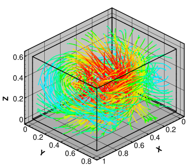
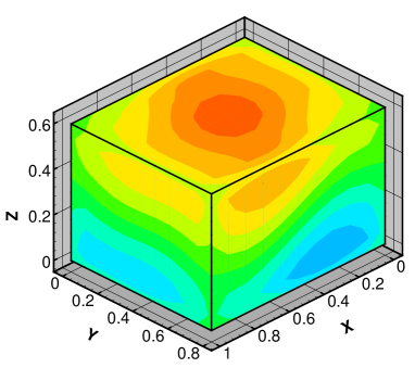
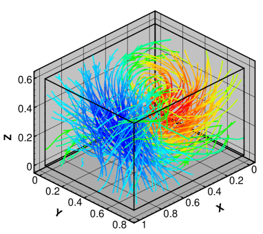
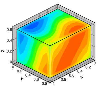
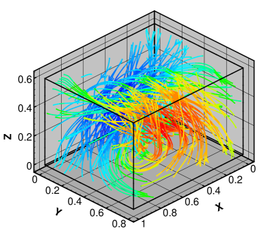
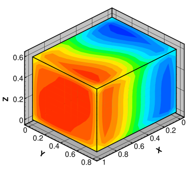
Figure 9: Magnetic fields within the box (left) and electric potentials at the box boundary (right) belonging to the three lowest eigenvalues of the $\alpha^{2}$ dynamo in a box with sidelengths ratio 1:0.8:0.6. The corresponding eigenvalues of $C$ are 4.728 (top), 4.898 (middle), and 4.934 (bottom). Evidently, the eigenmode with the dipole axis perpendicular to the largest box face (top) is most easily excitable.

For the particular case of a rectangular box with the sidelengths ratio 1.0:0.8:0.6 and a grid number $N=11$ we have visualized the magnetic fields and electric potentials belonging to the three lowest eigenvalues (Fig. 9). The structure of the magnetic field with its typical mixture of poloidal and toroidal components is clearly visible. It becomes evident that the field with the dipole axis perpendicular to the largest box face has the lowest eigenvalue.

It should be noted that we have also checked the divergence-free condition of the fields and the curl-free condition in the exteriour. Both conditions are fulfilled by the integral equation method with a reasonable accuracy.

V Conclusions

We have used the integral equation method to solve numerically the steady kinematic $\alpha^{2}$ dynamo problem in finite domains.

For spherical domains, our approach is similar to the integral equation method for the solution of the radial Schrödinger equation. In this case, with only some tens of grid points the method provides reasonable results for all three considered example profiles $\alpha(r)$. The error decreases with the inverse squared number of grid points. With the use of a convergence accelerating strategy, the accuracy and the convergence rate can be significantly improved. Interestingly, even oscillating solutions of the dynamo problem which cannot be reproduced by our steady method are at least mirrored by complex eigenvalues for the dynamo numbers whose real part is close to the correct critical value.

The particular suitability of the method to handle dynamos in arbitrarily shaped domains was demonstrated by the treatment of an $\alpha^{2}$ dynamo in rectangular boxes.

In summary, the integral equation method seems to be an attractive tool for the treatment of hydromagnetic dynamo problems. The robustness and accuracy of the method encourages to generalize it to the unsteady case and to more complicated dynamo models.

VI Acknowledgements

This work was supported by Deutsche Forschungsgemeinschaft in frame of the Collaborative Research Center SFB 609.

VII Appendix: The handling of the singularities

In this appendix, we present the techniques to handle the singularities in the integrals appearing in Eqs. (7) and (8) in general and for the matchbox in particular. For the integral

$$\int_{D}\frac{{\mathbf{F}}({\mathbf{r^{\prime}}})\times({\mathbf{r}}-{\mathbf{r^{\prime}}})}{|{\mathbf{r}}-{\mathbf{r^{\prime}}}|^{3}}\;dV^{\prime},$$

with ${\mathbf{r}}$ belonging to $D$, we split the domain $D$ into two parts, one being a small subdomain $D_{\epsilon}$ which is usually defined as a ball of a radius $\epsilon$ centered at ${\bf{r}}$, the remaining being the region $D-D_{\epsilon}$. Hence the integral can be decomposed according to

$${}\int_{D}\frac{{\mathbf{F}}({\mathbf{r^{\prime}}})\times({\mathbf{r}}-{\mathbf{r^{\prime}}})}{|{\mathbf{r}}-{\mathbf{r^{\prime}}}|^{3}}\;dV^{\prime} = \int_{D-D_{\epsilon}}\frac{{\mathbf{F}}({\mathbf{r^{\prime}}})\times({\mathbf{r}}-{\mathbf{r^{\prime}}})}{|{\mathbf{r}}-{\mathbf{r^{\prime}}}|^{3}}\;dV^{\prime}$$ (64)

$$+\int_{D_{\epsilon}}\frac{{\mathbf{F}}({\mathbf{r^{\prime}}})\times({\mathbf{r}}-{\mathbf{r^{\prime}}})}{|{\mathbf{r}}-{\mathbf{r^{\prime}}}|^{3}}\;dV^{\prime}.$$

The first integral of the right hand side of this equation is a normal integral without any singularity. For the second integral, the introduction of the spherical coordinates system $(\rho,\theta,\phi)$ leads to

$${}\int_{D_{\epsilon}}\frac{{\mathbf{F}}({\mathbf{r^{\prime}}})\times({\mathbf{r}}-{\mathbf{r^{\prime}}})}{|{\mathbf{r}}-{\mathbf{r^{\prime}}}|^{3}}\;dV^{\prime}= \int_{0}^{\epsilon}\int_{0}^{\pi}\int_{0}^{2\pi}{\bf{F}}(\rho,\theta,\phi)\times(\sin\theta\;\cos\phi,\sin\theta\;\sin\phi,\cos\theta)^{T}\;$$ (65)

$$\sin\theta\;d\phi\;d\theta\;d\rho$$

Assuming that the function ${\bf{F}}(\rho,\theta,\phi)$ is finite we see that the right hand side of Eq. (65) vanishes in the limit $\epsilon\rightarrow 0$.

Therefore, the considered singularity is a weak singularity. In order to avoid such a singularity in the numerical computation, we can just discretize the region $D-D_{\epsilon}$ instead of $D$. The error caused by this procedure can be made as small as desired by taking a small enough value of $\epsilon$. The same procedure can be applied to the first integral on the right hand side of Eq. (8) in the case $\bf{s}=\bf{r^{\prime}}$.

For the integral

$${}\int\limits_{S}\varphi({\mathbf{s^{\prime}}}){\mathbf{n}}({\mathbf{s^{\prime}}})\cdot\frac{{\mathbf{s}}-{\mathbf{s^{\prime}}}}{{|{\mathbf{s}}-{\mathbf{s^{\prime}}}|}^{3}}\;dS^{\prime},$$

appearing in Eq. (8), with ${\mathbf{s}}$ on the surface $S$, note that the unit vector ${\mathbf{n}}({\mathbf{s}}^{\prime})$ tends to be perpendicular to the vector ${\mathbf{s}}-{\mathbf{s}}^{\prime}$ in the case that ${\mathbf{s}}\rightarrow{\mathbf{s}}^{\prime}$, that is, ${\mathbf{n}}({\mathbf{s}}^{\prime})\cdot({\mathbf{s}}-{\mathbf{s}}^{\prime})$ tends to be zero. If defining $S_{\epsilon}$ as a small surface of a size $\epsilon$ including the point ${\mathbf{s}}$, we obtain BREB (p. 69):

$${}\lim_{\epsilon\to 0}\int\limits_{S_{\epsilon}}\varphi({\mathbf{s^{\prime}}}){\mathbf{n}}({\mathbf{s^{\prime}}})\cdot\frac{{\mathbf{s}}-{\mathbf{s^{\prime}}}}{{|{\mathbf{s}}-{\mathbf{s^{\prime}}}|}^{3}}\;dS^{\prime}\rightarrow 0.$$ (66)

A similar strategy as mentioned above can be employed to avoid such a singularity by discretizing the surface $S-S_{\epsilon}$ instead of $S$.

Now we consider the integral

$${}\int_{S}\varphi({\mathbf{s^{\prime}}}){\mathbf{n}}({\mathbf{s^{\prime}}})\times\frac{{\mathbf{r}}-{\mathbf{s^{\prime}}}}{|{\mathbf{r}}-{\mathbf{s^{\prime}}}|^{3}}\;dS^{\prime},$$ (67)

with the point ${\mathbf{r}}$ sitting on the surface $S$. Denote $S_{\epsilon}$ as a small piece of the surface $S$, which satisfies $|{\mathbf{s}}^{\prime}-{\mathbf{r}}|<\epsilon$. Then the integral (67) can be written as

$${}\int_{S}\varphi({\mathbf{s^{\prime}}}){\mathbf{n}}({\mathbf{s^{\prime}}})\times\frac{{\mathbf{r}}-{\mathbf{s^{\prime}}}}{|{\mathbf{r}}-{\mathbf{s^{\prime}}}|^{3}}\;dS^{\prime}= \int_{S-S_{\epsilon}}\varphi({\mathbf{s^{\prime}}}){\mathbf{n}}({\mathbf{s^{\prime}}})\times\frac{{\mathbf{r}}-{\mathbf{s^{\prime}}}}{|{\mathbf{r}}-{\mathbf{s^{\prime}}}|^{3}}\;dS^{\prime}$$ (68)

$$+\int_{S_{\epsilon}}\varphi({\mathbf{s^{\prime}}}){\mathbf{n}}({\mathbf{s^{\prime}}})\times\frac{{\mathbf{r}}-{\mathbf{s^{\prime}}}}{|{\mathbf{r}}-{\mathbf{s^{\prime}}}|^{3}}\;dS^{\prime}.$$

The first integral of the right hand side of this equation is a normal integral with no singularity. As for the second, defining another small disk of a small enough radius $\eta$ centered at $\mathbf{r}$, we have

$$\lim_{\epsilon\to 0}\int_{S_{\epsilon}}\varphi({\mathbf{s^{\prime}}}){\mathbf{n}}({\mathbf{s^{\prime}}})\times\frac{{\mathbf{r}}-{\mathbf{s^{\prime}}}}{|{\mathbf{r}}-{\mathbf{s^{\prime}}}|^{3}}\;dS^{\prime} = \lim_{\epsilon\to 0}\;\lim_{\epsilon\to 0}\int_{S_{\epsilon}-S_{\eta}}\varphi({\mathbf{s^{\prime}}}){\mathbf{n}}({\mathbf{s^{\prime}}})\times\frac{{\mathbf{r}}-{\mathbf{s^{\prime}}}}{|{\mathbf{r}}-{\mathbf{s^{\prime}}}|^{3}}\;dS^{\prime}$$

$$= \varphi({\mathbf{r}}){\mathbf{n}}({\mathbf{r}})\times\lim_{\epsilon\to 0}\;\lim_{\eta\to 0}\int_{S_{\epsilon}-S_{\eta}}\frac{{\mathbf{r}}-{\mathbf{s^{\prime}}}}{|{\mathbf{r}}-{\mathbf{s^{\prime}}}|^{3}}\;dS^{\prime},$$

where $0<\eta<\epsilon$. Introducing the local polar coordinates, $dS^{\prime}=\rho d\theta d\rho$, leads to

$${}\lim_{\eta\to 0}\int_{S_{\epsilon}-S_{\eta}}\frac{{\mathbf{r}}-{\mathbf{s^{\prime}}}}{|{\mathbf{r}}-{\mathbf{s^{\prime}}}|^{3}}\;dS^{\prime} = -\lim_{\eta\to 0}\int_{\eta}^{\epsilon}\frac{1}{\rho}d\rho\int_{0}^{2\pi}(\cos\theta,\sin\theta)^{T}d\theta$$ (69)

$$= -\lim_{\eta\to 0}\ln\frac{\epsilon}{\eta}\int_{0}^{2\pi}(\cos\theta,\sin\theta)^{T}d\theta.$$

Since the integrals $\int_{0}^{2\pi}\cos\theta\;d\theta$ and $\int_{0}^{2\pi}\sin\theta\;d\theta$ always vanish, we have

$${}\lim_{\eta\to 0}\int_{S_{\epsilon}-S_{\eta}}\frac{{\mathbf{r}}-{\mathbf{s^{\prime}}}}{|{\mathbf{r}}-{\mathbf{s^{\prime}}}|^{3}}\;dS^{\prime}=0.$$ (70)

Therefore,

$${}\lim_{\epsilon\to 0}\int_{S_{\epsilon}}\varphi({\mathbf{s^{\prime}}}){\mathbf{n}}({\mathbf{s^{\prime}}})\times\frac{{\mathbf{r}}-{\mathbf{s^{\prime}}}}{|{\mathbf{r}}-{\mathbf{s^{\prime}}}|^{3}}\;dS^{\prime}=0.$$ (71)

This indicates that we can also discretize the surface $S-S_{\epsilon}$ instead of $S$ in order to avoid such a singularity in the numerical computation.

For more details of the handling of the various singularities, one may refer to PARI (pp. 7-16).

References

• (1) K. Atkinson, The Numerical Solution of Integral Equations of the Second Kind (Cambridge University Press, Cambridge, 1997).
• (2) A. C. L. Barnard, I. M. Duck, M. S. Lynn, and W. P. Timlake, The application of electromagnetic theory to electrocardiography. II. Numerical solution of the integral equations, Biophys. J. 7, 463-491 (1967).
• (3) C. A. Brebbia, J. C. F. Telles and L. C. Wrobel, Boundary Element Techniques (Springer, Berlin, 1984).
• (4) E. Buendia, R. Guardiola, and M. Montoya, Integral Equations: A Tool to Solve the Schrödinger Equation, J. Comput. Phys. 68, 187-201 (1987).
• (5) A. Brandenburg, Å. Nordlund, R. F. Stein, and Torkelsson, Dynamo-generated turbulence and large scale magnetic fields in a Keplerian shear flow, ApJ 446, 741–754 (1995).
• (6) W. Dobler and K.-H. Rädler, An integral equation approach to kinematic dynamo models, Geophys. Astrophys. Fluid Dyn. 89, 45-74 (1998).
• (7) T. H. Christopher and M. A. Baker, The Numerical Treatment of Integral Equations (Clarendon Press, Oxford, 1977).
• (8) L. M. Delves and J. Walsh, Numerical Solution of Integral Equations (Clarendon Press, Oxford, 1974).
• (9) L. M. Delves and J. L. Mohamed, Computional methods for integral equations (Cambridge University Press, Cambridge, 1985).
• (10) Ya. Freiberg, Optimization of the shape of the toroidal model of an MHD dynamo, Magnetohydrodynamics 11, No 3, 269-272 (1975).
• (11) A. Gailitis, Self-excitation of a magnetic field by a pair of annular vortices, Magnetohydrodynamics 6, No 1, 14-17 (1970).
• (12) A. Gailitis and Ya. Freiberg, Self-excitation of a magnetic field by a pair of annular eddies, Magnetohydrodynamics 10, No 1, 26-30 (1974).
• (13) A. Gailitis, O. Lielausis, S. Dement’ev, E. Platacis, A. Cifersons, G. Gerbeth, Th. Gundrum, F. Stefani, M. Christen, H. Hänel, and G. Will, Detection of a flow induced magnetic field eigenmode in the Riga dynamo facility, Phys. Rev. Lett. 84, 4365-4368 (2000).
• (14) A. Gailitis, O. Lielausis, E. Platacis, S. Dement’ev, A. Cifersons, G. Gerbeth, Th. Gundrum, F. Stefani, M. Christen, and G. Will, Magnetic field saturation in the Riga dynamo experiment, Phys. Rev. Lett. 86, 3024-3027 (2001).
• (15) A. Gailitis, O. Lielausis, E. Platacis, G. Gerbeth, and F. Stefani., Laboratory Experiments on Hydromagnetic Dynamos, Rev. Mod. Phys. 74, 973-990 (2002).
• (16) R. A. Gonzales, J. Eisert, I. Koltracht, M. Neumann, and G. Rawitscher, Integral equation method for the continuous spectrum radial Schrödinger equation, J. Comp. Phys. 134, 134-149 (1997).
• (17) R. A. Gonzales, S.-Y. Kang, I. Koltracht, and G. Rawitscher, Integral equation method for coupled Schrödinger equations, J. Comp. Phys. 153, 160 - 202 (1999).
• (18) L. Greengard and V. Rokhlin, On the Numerical Solution of Two-Point Boundary Value Problems, Comm. Pure Appl. Math 44, 419–452 (1991).
• (19) W. Hackbusch, Integral Equations: Theory and Numerical Treatment (Springer, Berlin, 1995).
• (20) M. Hämäläinen, R. Hari, R. J. Ilmoniemi, J. Knuutila, O. V. Lounasmaa, Magnetoencephalography - theory, instrumentation, and application to noninvasive studies of the working human brain, Rev. Mod. Phys. 65, 413–497 (1993).
• (21) F. Krause and K.-H. Rädler, Mean-field Magnetohydrodynamics and Dynamo Theory (Akademie-Verlag, Berlin, 1980).
• (22) F. Krause and M. Steenbeck, Untersuchung der Dynamowirkung einer nichtspiegelsymmetrischen Turbulenz an einfachen Modellen, Z. Naturforsch. 22a, 671-675 (1967).
• (23) A. J. Meir and P. G. Schmidt, Analysis and numerical approximation of a stationary MHD flow problem with non-ideal boundary, SIAM J. Numer. Anal. 36, 1304 (1999).
• (24) H. K. Moffatt, Magnetic field generation in electrically conducting fluids (Cambridge University Press, Cambridge, 1978).
• (25) U. Müller and R. Stieglitz, Can the Earth’s magnetic field be simulated in the laboratory?, Naturwissenschaften 87, 381-390 (2000).
• (26) F. París and J. Cañas, Boundary Element Method (Fundamentals and Applications) (Oxford University Press, 1997).
• (27) W. H. Press, S. A. Teukolsky, W. T. Vetterling, B. F. Flannery, Numerical Recipes (Cambridge University Press, Cambridge, 1992).
• (28) K.-H. Rädler, E. Apstein, M. Rheinhardt, and M. Schüler, The Karlsruhe dynamo experiment - a mean-field approach, Studia geoph. et geod. 42, 224-231 (1998).
• (29) K.-H. Rädler, M. Rheinhardt, E. Apstein, and H. Fuchs, On the mean-field theory of the Karlsruhe dynamo experiment, Nonlinear Proc. Geoph. 9, 171-187 (2002)
• (30) P. H. Roberts, An Introduction to Magnetohydrodynamics (Elsevier, New York, 1967).
• (31) G. Rüdiger and Y. Zhang, MHD instability in differentially-rotating cylindric flows. Astron. Astrophys. 378, 302-308 (2001).
• (32) F. Stefani, G. Gerbeth, and A. Gailitis, Velocity profile optimization for the Riga dynamo experiment, in Transfer Phenomena in Magnetohydrodynamics and Electroconducting Flows, edited by A. Alemany, Ph. Marty, and J.-P. Thibault, 31-44 (Kluwer, Dordrecht, 1999).
• (33) F. Stefani, G. Gerbeth, and K.-H. Rädler, Steady dynamos in finite domains: an integral equation approach, Astron. Nachr. 321, 65-73 (2000).
• (34) F. Stefani and G. Gerbeth, G., Oscillatory mean-field dynamos with a spherically symmetric, isotropic helical turbulence parameter $\alpha$, Phys. Rev. E 67, 027302 (2003)
• (35) R. Stieglitz and U. Müller, U., Experimental demonstration of a homogeneous two-scale dynamo, Phys. Fluids 13, 561-564 (2001).