The trispectrum of the Cosmic Microwave Background on sub-degree angular scales: an analysis of the BOOMERanG data

Abstract

The trispectrum of the cosmic microwave background can be used to assess the level of non-Gaussianity on cosmological scales. It probes the fourth order moment, as a function of angular scale, of the probability distribution function of fluctuations and has been shown to be sensitive to primordial non-gaussianity, secondary anisotropies (such as the Ostriker-Vishniac effect) and systematic effects (such as astrophysical foregrounds). In this paper we develop a formalism for estimating the trispectrum from high resolution sky maps which incorporates the impact of finite sky coverage. This leads to a series of operations applied to the data set to minimize the effects of contamination due to the Gaussian component and correlations between estimates at different scales. To illustrate the effect of the estimation process, we apply our procedure to the BOOMERanG data set and show that it is consistent with Gaussianity. This work presents the first estimation of the CMB trispectrum on sub-degree scales.

1 Introduction

The Cosmic Microwave Background (CMB) has become the observational tool of excellence for probing the statistical nature of inhomogeneities in the universe. The small deviations from homogeneity which have been detected by over two dozen different experiments can be directly related to the primordial origin of perturbations in the early universe and therefore to fundamental physics at very high energies. A new threshold was crossed in the experimental forum with the high resolution, high sensitivity mapping of significant fractions of the CMB sky by the BOOMERanG (de Bernardis et al. 2000) and MAXIMA (Hanany et al. 2000) experiments. A careful analysis of the variance of fluctuations in these maps has led to accurate estimates of the angular power spectrum, far surpassing previous experimental analyses on small angular scales. More recent results from BOOMERanG (Netterfield et al. 2002, Ruhl et al. 2002), MAXIMA (Lee et al. 2001), and from other experiments like DASI (Halverson et al. 2002), CBI (Pearson et al. 2002), VSA (Grainge et al. 2002), ACBAR (Kuo et al. 2002) and ARCHEOPS (Benoit et al. 2002) have posed our knowledge of the CMB angular power spectrum on even more solid ground. However, there is more information in the CMB fluctuations than what is provided by its power spectrum alone. The standard way to extract this information is to analyse high signal to noise maps of the CMB field like those already produced by BOOMERanG or the ones that the MAP satellite is expected to provide shortly.

There is, therefore, strong motivation to attempt a more detailed study of the CMB sky; in principle one would like a complete characterisation of the probability distribution function of the fluctuations in the CMB with the hope that it might probe more fundamental features of the origin of structure in the universe. For example one relatively stringent test of whether the origin of fluctuations is due to a standard, single-field inflationary model is if the CMB is a realization of a nearly Gaussian distribution [Coles and Barrow 1987], while other models like the curvaton might lead to a much larger non-Gaussian contribution [Lyth & Wands 2002, Bartolo & Liddle 2002, Bernardeau & Uzan 2002, Bernardeau & Uzan 2002]. Many secondary anisotropies like the Ostriker-Vishniac (OV) effect [Ostriker & Vishniac 1986] and the Sunyaev-Zeldovich effect [Sunyaev & Zeldovich 1980] can introduce measurable non-Gaussianity while foregrounds and systematics may contribute as well.

A standard method of parametrising an arbitrary probability distribution function is in terms of all its higher order moments. In the case of statistically homogeneous and isotropic fields it is more convenient to consider moments of the Fourier transform of the field; these symmetries will impose a set of selection rules which pick out the true degrees of freedom. The past few years have seen initial attempts at constraining these moments by measuring them with the available data. A series of analyses of the bispectrum (the cubic moment) of the COBE data have revealed the presence of a non-Gaussian systematic [Ferreira, Magueijo, & Gorski 1998, Banday, Zaroubi & Gorski 2000, Komatsu et al. 2001]. This has been confirmed with an analysis of the trispectrum, the quartic moment [Kunz et al 2001, Komatsu 2002]. But no primordial non-Gaussianity was detected. On smaller angular scales analyses of the QMAP and QMASK[Park et al. 2001] and MAXIMA [Wu et al 2001, Santos et al 2002] data have shown that their observations are consistent with the assumption that the CMB anisotropies are the result of an isotropic Gaussian random process. The analyses of these data sets have also revealed that statistical methods may be sensitive to the data processing pipeline. Moreover, different technical issues must be confronted if one is considering finite sky coverage as opposed to full sky coverage.

The trispectrum, which we consider in this study, probes a rather different kind of non-Gaussianity than the bispectrum; [Aghanim et al 2003] found it to be very sensitive to point sources and [Castro 2003] showed it to be a powerful probe of the OV effect. It can also be used to detect weak lensing in the CMB [Cooray & Kesden 2002]. In particular, as described in [Bernardeau 1997], weak lensing does not introduce a three-point correlation function, meaning that its expected bispectrum is zero. The first non trivial higher order correlation function to detect weak lensing effects is the trispectrum. Using the trispectrum to test for non-Gaussianity in high-resolution CMB maps complements therefore other analyses using the bispectrum, like [Santos et al 2002]. The purpose of this paper is to improve, extend and apply the method for estimating the trispectrum first proposed in Kunz et al (2001) where it was applied to the full sky map produced by the COBE satellite.

Using techniques developed for performing the operation in pixel space [Ferreira, Magueijo, & Silk 1997, Spergel & Goldberg 1999, Hu 2001] we present a formalism which can easily be extended to high $\ell$s and discuss a robust method for identifying an orthogonal set of estimators in the full-sky case. We then discuss the various numerical and statistical problems one faces when analysing finite sky coverage. We finally use the BOOMERanG data as a test case to extract the first estimate of the trispectrum on sub-degree angular scales.

2 Formalism and Notation

In this section we present the notation that will be used throughout this work. We start with a temperature anisotropy field defined on the sphere, $\frac{\Delta T}{T}({\bf n})$; it may be expanded in terms of spherical harmonic functions, $Y_{\ell m}({\bf n})$:

$$\frac{\Delta T}{T}({\bf n})=\sum_{\ell m}a_{\ell m}Y_{\ell m}({\bf n}).$$ (1)

For any theory of structure formation, the $a_{\ell m}$ coefficients are a set of random variables; we shall restrict ourselves to theories which are statistically homogeneous and isotropic. The power spectrum $C_{\ell}$ of the temperature anisotropies is then defined by

$$\langle a_{\ell m}a^{*}_{\ell^{\prime}m^{\prime}}\rangle=C_{\ell}\delta_{\ell\ell^{\prime}}\delta_{mm^{\prime}}.$$ (2)

If we consider the 3-point function of the temperature field, we obtain the bispectrum, defined as

$$\langle a_{\ell_{1}m_{1}}a_{\ell_{2}m_{2}}a_{\ell_{3}m_{3}}\rangle=\left(\begin{array}[]{ccc}\ell_{1}&\ell_{2}&\ell_{3}\\ m_{1}&m_{2}&m_{3}\end{array}\right)B_{\ell_{1}\ell_{2}\ell_{3}}.$$ (5)

The term ($\cdots$) is a Wigner 3J symbol, which arises due to the “selection rules” of the moments.

Following the same steps, we can construct the 4-point function and the associated trispectrum. We represent the rotationally invariant solution for the trispectrum as in [Hu 2001]:

$$\langle a_{\ell_{1}m_{1}}a_{\ell_{2}m_{2}}a_{\ell_{3}m_{3}}a_{\ell_{4}m_{4}}\rangle=\sum_{LM}\left(\begin{array}[]{ccc}\ell_{1}&\ell_{2}&L\\ m_{1}&m_{2}&-M\end{array}\right)\left(\begin{array}[]{ccc}\ell_{3}&\ell_{4}&L\\ m_{3}&m_{4}&M\end{array}\right)(-1)^{M}Q^{\ell_{1}\ell_{2}}_{\ell_{3}\ell_{4}}(L)$$ (10)

Using the orthogonality properties of the Wigner 3J symbols and the relation $Q=T+G$, we can invert the equation (10) to obtain the estimator

$$\hat{T}^{\ell_{1}\ell_{2}}_{\ell_{3}\ell_{4}}(L)=(2L+1)\sum_{m_{1}m_{2}m_{3}m_{4}M}(-1)^{M}\left(\begin{array}[]{ccc}\ell_{1}&\ell_{2}&L\\ m_{1}&m_{2}&M\end{array}\right)\left(\begin{array}[]{ccc}\ell_{3}&\ell_{4}&L\\ m_{3}&m_{4}&-M\end{array}\right)\times$$ (15)

$$a_{\ell_{1}m_{1}}a_{\ell_{2}m_{2}}a_{\ell_{3}m_{3}}a_{\ell_{4}m_{4}}-\hat{G}_{l_{3}l_{4}}^{l_{1}l_{2}}(L)$$

The term $G_{l_{3}l_{4}}^{l_{1}l_{2}}(L)$ represents the unconnected Gaussian contribution and it is given in (Hu 2001) as:

$$G_{l_{3}l_{4}}^{l_{1}l_{2}}(L)=(-1)^{(l_{1}+l_{3})}\sqrt{(2l_{1}+1)(2l_{3}+1)}C_{l_{1}}C_{l_{3}}\delta_{l_{1}l_{2}}\delta_{l_{3}l_{4}}\delta_{L0}+(2L+1)C_{l_{1}}C_{l_{2}}\times$$ (16)

$$[(-1)^{l_{2}+l_{3}+L}\delta_{l_{1}l_{3}}\delta_{l_{2}l_{4}}+\delta_{l_{1}l_{4}}\delta_{l_{2}l_{3}}]$$

The term $\hat{T}^{\ell_{1}\ell_{2}}_{\ell_{3}\ell_{4}}(L)$ is the connected part of the angular trispectrum and its expectation value is exactly zero for a Gaussian field. This means that the connected part is sensitive to the presence of non Gaussianities. The unconnected term is non-zero only for $L=0$ or $l_{1}=l_{2}=l_{3}=l_{4}$, but only with full sky coverage. In the case of incomplete sky coverage the unconnected terms can contaminate all other modes. We will discuss this situation in section (3).

For the purpose of this work we have not computed the possible trispectrum components. We concentrated only on the simpler case $\ell_{1}=\ell_{2}=\ell_{3}=\ell_{4}=\ell$, i.e. the diagonal component. Recent papers have investigated in detail the power of the diagonal trispectrum in the presence of some non-Gaussian signals mentioned in the introduction. In particular, [Aghanim et al 2003] has shown that for simulated point-source maps the diagonal trispectrum is much more powerful than the nearly diagonal estimator ($\ell,\ell+1,\ell+2,\ell+3$), even though the latter does not contain a Gaussian contribution. Also, in [Castro 2003] it is discussed how the OV effect generates a signature on the diagonal tispectrum which could easily be detected on the arcminute scales probed by the Planck mission.

Finally it should be noticed that computing all components of the trispectrum is a serious computational challenge. Many modes are also correlated due to the limited sky coverage. For these reasons we have decided to restrict this analysis to the case of $\ell_{1}=\ell_{2}=\ell_{3}=\ell_{4}=\ell$.

We start with the method described in [Kunz et al 2001]. We define

$$\langle a_{\ell m_{1}}a_{\ell m_{2}}a_{\ell m_{3}}a_{\ell m_{4}}\rangle=\sum_{a=0}^{n}T_{\ell;a}\tau_{m_{1}m_{2}m_{3}m_{4}}^{a;\ell}$$ (17)

where the $T_{\ell,a}$ are the components of the trispectrum that we wish to estimate, and $\tau$ is a tensor which we have to determine in order to construct an estimator for $T_{\ell,a}$. The geometrical considerations stated above, together with the required symmetries with respect to the interchange of $\{\ell_{i},m_{i}\}$ pairs suggest

$$\bar{\tau}_{m_{1}m_{2}m_{3}m_{4}}^{\alpha,\ell}=\sum_{M=-2\alpha}^{2\alpha}(-1)^{M}\left(\begin{array}[]{ccc}\ell&\ell&2\alpha\\ m_{1}&m_{2}&M\end{array}\right)\left(\begin{array}[]{ccc}2\alpha&\ell&\ell\\ -M&m_{3}&m_{4}\end{array}\right)+\mathrm{ineq.permut.}$$ (22)

Although the $\bar{\tau}$s satisfy all the correct symmetries, they define an over-complete basis. To correct for this deficiency we define an orthonormalised set of tensors

$$\tau_{m_{1}m_{2}m_{3}m_{4}}^{a;\ell}=\sum_{\alpha=0}^{\ell}{\cal L}_{\ell}^{a\alpha}\bar{\tau}_{m_{1}m_{2}m_{3}m_{4}}^{\alpha,\ell},$$ (23)

where the matrix ${\cal L}_{\ell}^{a\alpha}$ is derived from the required property that the $\tau$ be orthogonal with respect to the product given in equation (5) of Kunz et al (2001). The estimator of the trispectrum is then given by

$$\hat{T}_{\ell;a} = \sum_{m_{1}m_{2}m_{3}m_{4}}{\tau}^{a;\ell}_{m_{1}m_{2}m_{3}m_{4}}a_{\ell m_{1}}a_{\ell m_{2}}a_{\ell m_{3}}a_{\ell m_{4}}$$

$$= \sum_{m_{i}}\sum_{\alpha=0}^{\ell}{\cal L}^{a;\alpha}_{\ell}\bar{\tau}^{\alpha;\ell}_{m_{1}m_{2}m_{3}m_{4}}a_{\ell m_{1}}a_{\ell m_{2}}a_{\ell m_{3}}a_{\ell m_{4}}$$

$$\equiv \sum_{\alpha=0}^{\ell}{\cal L}^{a;\alpha}_{\ell}\bar{T}^{\alpha;\ell}$$

Note that there are only ${\rm int}(\ell/3)$ independent estimators due to the symmetry properties of the $a_{\ell m}$. In this paper we will consider the “normalised” trispectrum used in Kunz et al (2001) where we divide each estimate of the trispectrum by $({\hat{C}}_{\ell})^{2}$, where ${\hat{C}}_{\ell}=\frac{1}{2\ell+1}|a_{\ell m}|^{2}$. Its statistical properties are equivalent to the ones of the unnormalised estimator, and it is more robust with respect to fluctuations in the power spectrum [Aghanim et al 2003].

3 Application to high resolution maps with incomplete sky coverage

In this paper we will be focusing on a high-resolution map with incomplete sky coverage, in particular the BOOMERanG data set. This leads to a set of algorithmic problems which did not have to be addressed in Kunz et al (2001). The three problems we wish to highlight are:

Speed:

The numerical evaluation of Wigner 3J coefficients for large values of $\ell$ becomes time consuming and practically unfeasible. Indeed beyond the COBE resolution of a maximum $\ell$ of approximately 25 it is not possible to estimate the $\bar{T}^{\alpha;\ell}$ sufficiently rapidly for a robust Monte Carlo assessment of the statistics.

Gaussian Contamination:

The finite sky coverage will induce correlations between the estimators with different values of $\ell$ and $a$ (or $\alpha$). As a consequence, all estimators may be heavily contaminated by the Gaussian (or disconnected) contributions to the maps.

Correlations:

The correlations between modes in the cut sky mean that the $\bar{T}^{\alpha;\ell}$ will be even more correlated than in the full sky case.

We shall now focus on the solutions we propose to these three problems

3.1 Speed

We have opted to use the method described in [Hu 2001, Spergel & Goldberg 1999] for calculating $\bar{T}^{\alpha;\ell}$: we define a new set of sky maps weighted in rings centred around a point $\hat{\bf q}$:

$$e_{\ell}(\hat{\bf q})=\sqrt{\frac{2\ell+1}{4\pi}}\int{d\hat{\bf n}T(\hat{\bf n})P_{\ell}(\hat{\bf n}\cdot\hat{\bf q}})$$ (25)

To implement this method we start with the relation (25) and we use the relation (1) to express the temperature $T$ as a function of spherical harmonics and the relation:

$$P_{\ell}(\hat{\bf n}\cdot\hat{\bf q})=\frac{4\pi}{2\ell+1}\sum_{m}Y_{\ell m}^{\ast}(\hat{\bf n})Y_{\ell m}(\hat{\bf q})$$ (26)

to express also the Legendre polynomials as a function of spherical harmonics. Combining them with equation (25) we obtain:

$$e_{\ell}(\hat{\bf q})=\sqrt{\frac{4\pi}{2\ell+1}}\sum_{m}a_{\ell m}Y_{\ell m}(\hat{\bf q})$$ (27)

The $e_{\ell}$ calculation is quite fast because we can use the fast Fourier transform on rings of equal latitude (Muciaccia et al 1997).

We can then rewrite equation (15) in terms of this new set of sky maps (Komatsu 2002):

$$\bar{T}^{\alpha;\ell}=\frac{1}{4\alpha+1}\sum_{M=-2\alpha}^{2\alpha}t_{2\alpha,M}^{\ell\ell\ast}t_{2\alpha,M}^{\ell\ell}$$ (28)

where

$$t_{LM}^{\ell\ell}=\sqrt{\frac{2L+1}{4\pi}}\left(\begin{array}[]{ccc}\ell&\ell&L\\ 0&0&0\end{array}\right)^{-1}\int{d\hat{\bf n}}{[e_{\ell}(\hat{\bf n})e_{\ell}(\hat{\bf n})]Y^{\ast}_{LM}(\hat{\bf n})}$$ (31)

If we expand the Wigner 3J symbols in terms of spherical harmonics and use the addition theorem we obtain:

$$\bar{T}^{\alpha;l}=N^{-1}_{\ell 2\alpha}\int{\frac{d^{2}\hat{n}}{4\pi}}\int{\frac{d^{2}\hat{q}}{4\pi}e_{\ell}(\hat{n})e_{\ell}(\hat{n})e_{\ell}(\hat{q})e_{\ell}(\hat{q})P_{2\alpha}(\hat{n}\cdot\hat{q})}$$ (32)

where

$$N_{\ell L}=\frac{1}{3}\left(\begin{array}[]{ccc}\ell&\ell&L\\ 0&0&0\end{array}\right)^{2}$$ (35)

We have thus computed a set of $\bar{T}^{\alpha;\ell}$ which we can orthonormalise to get the estimator for the trispectrum $\hat{T}^{a;\ell}$. This method is very fast, especially when estimating the trispectrum at high values of $\ell$. Note that direct evaluation of the Wigner 3J coefficients, e.g. by recurrence relations, would result in an ${\cal O}(\ell^{5})$ problem, requiring $\sim 10^{16}$ operations for $\ell\sim 1000$.

3.2 Gaussian Contamination

Kunz et al (2001) found that the purely Gaussian contribution to the trispectrum (the disconnected part) corresponds to the $\alpha=0$ term. By orthogonalising all other estimators with respect to this tensor it is possible to remove the Gaussian contribution exactly on a map by map basis. The resulting estimators are only sensitive to non-Gaussian contributions, i.e. in the case of Gaussian skies they would have a zero expectation value. Additionally, the variance of this estimator is shown to be minimal [Kunz et al 2001]. In the cut sky case, there are strong cross correlations between components of the trispectrum with different values of $\ell$ and $\alpha$. In this case, the orthogonalisation method fails. Given that the Gaussian contribution to the trispectrum may be much larger than the non-Gaussian contribution, it is essential that we remove it as completely as possible nonetheless.

To overcome these problems we have chosen to employ the following Monte Carlo scheme: we generate an ensemble of maps with the same angular power spectrum, sky coverage and noise as the data maps we want to analyse. We estimate the $\bar{T}^{\alpha;\ell}$ from each map and calculate the mean of these quantities over the whole ensemble. Let us denote this mean by $\bar{T}^{\alpha;\ell}_{G}$. We then use this quantity to correct for the Gaussian contamination in the estimate of the trispectrum from the data by defining $\bar{T}^{\alpha;\ell}_{GC}=\bar{T}^{\alpha;\ell}-\bar{T}^{\alpha;\ell}_{G}$. Note that, by so doing, we are removing the Gaussian contamination before performing the full-sky orthogonalisation, i.e. before multiplying by ${\cal L}$.

3.3 Correlations

The fact that there is only limited sky coverage also implies that there will be correlations between values of the trispectrum at different $\ell$s. This is shown in section 5 below. To strongly suppress the correlations and to end up with a simple covariance matrix, we consider band averaged values of the trispectrum. Since there is no a priori given band width, we study the cases of $\Delta\ell=40$, $50$ and $60$ and $\Delta a=10$ and $15$. The choice $\Delta\ell\simeq 50$ is consistent with previous analyses of the BOOMERanG power spectrum (see, e.g., [Ruhl et al. 2002]). In this way we can check the sensitivity of the results to the chosen band size.

4 Numerical Implementation and Consistency Tests

The process we use is basically the same as in a number of previous analyses [Kogut et al 1996, Ferreira, Magueijo, & Gorski 1998, Kunz et al 2001, Santos et al 2002]. We generate an ensemble of Gaussian maps with the same angular power spectrum and noise property as estimated from the BOOMERanG data and the same sky coverage. We then apply our estimators to the set of maps to obtain a distribution for each estimator in the Gaussian case. In particular we characterise the full distribution in terms of the mean values of the estimators and the covariance matrix between them. These quantities are used to define a standard multivariate $\chi^{2}$ as a goodness of fit. The estimators of the trispectrum are then evaluated from the BOOMERanG data. In section 5 we will discuss their behaviour. The goodness of fit of these estimators is compared against its distribution for a new ensemble of Gaussian maps. From this comparison we can quantify the confidence with which the data can be said to be Gaussian from the point of view of our estimator. It is clear that the numerical details of this process must be well understood if we are to believe in our results. We focus on the particularities of the analysis in this paper which differ from previous analyses.

It is important to compare the results using this hybrid pixel/harmonic analysis with the standard methods which have been used before. We do so by looking at the two lower order statistics, i.e. we have calculated the power spectrum $C_{\ell}$ and the bispectrum $B_{\ell\ell\ell}$ using this new approach as well as summing up the 3J symbols. The relevant expressions are:

$$C_{\ell}=\frac{1}{4\pi}\int{d{\bf q}\left|e_{\ell}({\bf q})\right|^{2}}$$ (36)

and (Spergel et al. 1999)

$$\left(\begin{array}[]{ccc}\ell&\ell&\ell\\ 0&0&0\end{array}\right)B_{\ell\ell\ell}=\int{d{\bf q}e_{\ell}({\bf q})e_{\ell}({\bf q})e_{\ell}({\bf q})}$$ (39)

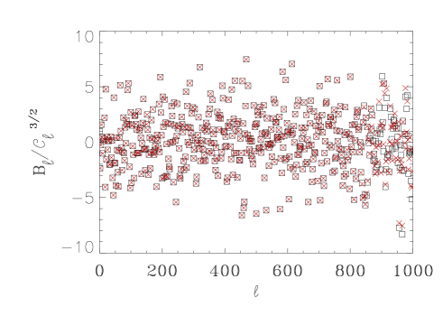
Figure 1: In this figure we represent the normalised bispectrum $I^{3}_{\ell}=B_{\ell}/C^{3/2}_{\ell}$ calculated for a full sky Gaussian map with a pixel size of $7^{{}^{\prime}}$. The red crosses show $I^{3}_{\ell}$ obtained with the $e_{\ell}$ method, the black boxes $I^{3}_{\ell}$ with $a_{\ell m}$ and the 3J symbols. We can see that at $\ell\simeq 800$ there is a quite evident difference between two plots, due to a pixelisation effect. We limit therefore our analysis to $\ell\leq 700$.

We have compared the $C_{\ell}$ and $B_{\ell\ell\ell}$ using these expressions with the standard results obtained using $a_{\ell m}$ and the Wigner 3J symbols, for a maximum $\ell$ value of $1000$. Using a set of CMB Gaussian maps with the best fit power spectrum measured by Boomerang [Netterfield et al. 2002] and a pixel resolution of $7^{{}^{\prime}}$ we have found that the bispectrum obtained with $e_{\ell}$ is affected by a pixelisation effect for high values of $\ell$ (while the power spectrum shows no difference). To check for this, we have done the same analysis with higher resolution ($\simeq 3^{{}^{\prime}}$) and have found that the pixelisation effect vanishes. Given that we are restricted to the pixelisation level of the data, we can use the comparison of the two estimates of the bispectrum to define a maximum $\ell$ out to which we can trust the new estimate of the trispectrum. Note that it is computationally intractable to perform such a comparison in terms of the trispectrum, although this would be preferable. From Fig. 1 one can see that discrepancies arise for $\ell>800$ and we chose not to estimate the trispectrum beyond $\ell=700$, leaving a conservative margin as we did not test the trispectrum itself. Furthermore, we chose not to consider any $\ell$ below 100 because the BOOMERanG data are not very sensitive to these modes, due to limited sky coverage and data filtering.

Another novelty in our analysis (as compared to that of Kunz et al. 2001) is the method for constructing ${\cal L}_{\ell}^{a;\alpha}$. There, a Gram-Schmidt (GS) procedure was used to calculate the orthonormal transformation matrix ${\cal L}_{\ell}^{a;\alpha}$. Due to the inherent instability of the GS procedure, it is not applicable to large matrices, i.e. for large $\ell$. We have opted therefore to use an alternative orthonormalisation method. We subtract the $a=0$ part and use a Jacobi routine to obtain a spectral decomposition (SD) of the remaining matrix. The eigenvectors of the non-vanishing eigenvalues form then the transformation matrices. This method is robust and, moreover, gives us an unambiguous procedure for ordering the estimators through the different eigenvalues. As a strong consistency test we have applied our trispectrum code to the COBE data and compared the results with those of [Kunz et al 2001]. The results of the SD method lie, up to a possible sign change, very close to the original ones (see figure 2). In any case, the statistical significance of the results (and the conclusions one can extract) are the same as in Kunz et al (2001). We advocate the use of the SD method from now on, even in the case of analyses limited to low $\ell$s.

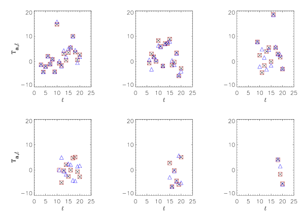
Figure 2: In this figure we reproduce the COBE results for the trispectrum with the GS and SD orthonormalisation methods (see text) and compare them with (Kunz et al. 2001).The black crosses are the (Kunz et al. 2001) results, green squares are GS method results and blue triangles are SD method results.

For our analysis we have used the best four of the six $150$ GHz channels of the BOOMERanG 1998 flight; we naively coadd the data taken at the scan speed of $1$ degree per second ($1$ dps). We simulate three sets of 1000 Gaussian maps each. In fact, we need three statistically independent ensembles of simulated maps for our analysis: one to estimate the Gaussian contribution described above, another to estimate our estimator’s covariance matrix and a third one to perform the actual comparison with real data. To produce the maps we follow the very same steps used during the real Boomerang data reduction. To generate a map we use timestream simulations created with the actual flight pointing and transient flagging. The signal component of these time streams is generated from simulated gaussian CMB maps, while the noise component is from gaussian realizations of the measured detector noise power spectrum. The noise spectrum is determined using the iterative procedure described in Ferreira $\&$ Jaffe (2000) and Netterfield et al. (2002).

To reduce the effects of $1/f$ noise on this naively binned map, a brick-wall highpass Fourier filter is first applied to the timestream at a frequency of $0.1$ Hz. A notch filter is also applied between 8 and 9 Hz to eliminate a non-stationary spectral line in the data. This only affects angular scales well above $\ell=1000$ and is therefore irrelevant for our analysis.

The coaddition of several channels is achieved by averaging the maps (both from the data, and from the Monte-Carlos of each channel). Each channel has a slightly different beam size, which is taken into account in the generation of the simulated maps. We select the most central region of the scan by applying an elliptical mask as in (Netterfield et al. 2002). This corresponds to $\simeq 1.8\%$ of the full sky. The mask selects a region of approximately uniform coverage and high signal to noise and comprises $\sim 57000$ pixels of size $\sim 7^{\prime}$ each in the Healpix pixelization scheme (Górski et al. 1998). We refer the reader to Ruhl et al. (2002) for a thorough description of a simulation pipeline (based on the MASTER/FASTER algorithms described in [Hivon et al. 2000]) very similar to the one used here.

5 Results and application to the BOOMERanG data

Figure 3: Top panel: An estimate of the non-orthogonalised trispectrum, ${\bar{T}}^{\alpha;\ell}$ (multiplied by $\ell^{4}$) for $\alpha=5,100,400$ from the BOOMERanG data (crosses) and the corresponding $95\%$ confidence limits from the $1000$ Monte-Carlo simulations. Bottom panel: An estimate of the non-orthogonalised trispectrum corrected for Gaussian contamination, ${\bar{T}}^{\alpha;\ell}$ (multiplied by $\ell^{4}$) for $\alpha=5,100,400$ from the BOOMERanG data (crosses) and the corresponding $95\%$ confidence limits from the $1000$ Monte-Carlo simulations.

To show in detail the method proposed in Sections 2 and 3 we are going to discuss the results obtained at each step from both the data and the Monte-Carlo simulations. We start with the estimate of the ${\bar{T}}^{\alpha;\ell}$ without Gaussian corrections. In the top panel of Figure 3 we plot ${\bar{T}}^{\alpha;\ell}$ as a function of $\ell$ for selected values of $\alpha$. We can highlight two features. Firstly the ${\bar{T}}^{\alpha;\ell}$ are highly correlated for adjacent values of $\ell$ due to the finite sky coverage, as expected. Secondly, and because of the finite sky coverage, there is a strong contamination from the disconnected component of the trispectrum. This is evident in the fact that the values of ${\bar{T}}^{\alpha;\ell}$ scatter about the $(C_{\ell})^{2}$ and that the $95\%$ confidence limits are not centred about zero. As one would expect the lower the value of $\alpha$, the more contaminated the estimate is by the disconnected part. As advocated in Section 3, we correct for the contamination due to the disconnected component by using a Monte Carlo ensemble (of 1000 realizations) to generate a correction. This can be seen as a bias which must be subtracted off all estimates of ${\bar{T}}^{\alpha;\ell}$ with $\alpha>0$. In the bottom panel of Figure 3 we plot the “Gaussian corrected” estimate of ${\bar{T}}^{\alpha;\ell}$ with corresponding $95\%$ confidence limits. As expected the estimates now scatter around zero, while the confidence limits, although not necessarily symmetric around the $\ell$ axis are much more centred. The remaining asymmetry is merely a manifestation that for low $\alpha$s the distribution of the ${\bar{T}}^{\alpha;\ell}$ is slightly skewed.

Figure 4: An estimate of the non-orthogonalised trispectrum corrected for Gaussian contamination and normalised ${\bar{T}}^{\alpha;\ell}/({\hat{C}}_{\ell})^{2}$ for $\alpha=5,100,400$ from the BOOMERanG data (crosses) and the corresponding $95\%$ confidence limits from the $1000$ Monte-Carlo simulations.

Given that we will be working with normalised estimates of the trispectrum (as in Kunz et al 2001) it is illustrative to plot the $\ell$ dependence of ${\bar{T}}^{\alpha;\ell}/({\hat{C}}_{\ell})^{2}$ for a few values of $\alpha$. We do this in Figure 4. One can see the dependence on $\alpha$ of the $95\%$ confidence intervals, i.e. the $\ell$ value of minimum scatter depends on $\alpha$.

Let us now proceed to the orthornomalised estimators, ${\hat{T}}_{a;\ell}$; a selection of estimators are plotted for a choice of $a$s in Figure 5. As noted above, the $a$ are limited to $a\leq{\rm int}(l/3)$, and we see a clear suppression of the high $a$ values for each $\ell$ (or, in the case of the figure, of the low $\ell$ values for fixed $a$), as the maps with limited sky coverage contain less information than full sky maps.

Figure 5: Top panel: An estimate of the orthogonalised trispectrum corrected for Gaussian contamination and normalised ${\hat{T}}_{a;\ell}/({\hat{C}}_{\ell})^{2}$ for $a=5,100,200$ from the BOOMERanG data (crosses) and the corresponding $95\%$ confidence limits from the $1000$ Monte-Carlo simulations. Bottom panel: The absolute value of the estimate of the orthogonalised trispectrum corrected for Gaussian contamination and normalised ${\hat{T}}_{a;\ell}/({\hat{C}}_{\ell})^{2}$ for $a=5,100,200$ from the BOOMERanG data (crosses) and the corresponding $95\%$ confidence limits from the $1000$ Monte-Carlo simulations.

Figure 6: The $\chi^{2}$ distribution of Monte-Carlo simulated maps (histogram) and data value (vertical line) for the trispectrum estimator $|{\hat{T}}_{a;\ell}|$ in the case of $\Delta a=10$ and $\Delta l=40,50,60$ (top) and in the case of $\Delta a=15$ and $\Delta l=40,50,60$ (bottom)

Figure 7: The $\chi^{2}$ distribution of Monte-Carlo simulated maps (histogram) and data value (vertical line) for the trispectrum estimator ${\hat{T}}_{a;\ell}$ in the case of $\Delta a=10$ and $\Delta l=40,50,60$ (top) and in the case of $\Delta a=15$ and $\Delta l=40,50,60$ (bottom)

bin width	$|{\hat{T}}_{a;\ell}|$	${\hat{T}}_{a;\ell}$
$\Delta\ell=40$
$\Delta a=10$	$21.8\%$	$10.6\%$
$\Delta\ell=50$
$\Delta a=10$	$13.7\%$	$19.3\%$
$\Delta\ell=60$
$\Delta a=10$	$76\%$	$23.2\%$
$\Delta\ell=40$
$\Delta a=15$	$15.7\%$	$26\%$
$\Delta\ell=50$
$\Delta a=15$	$8.7\%$	$8.5\%$
$\Delta\ell=60$
$\Delta a=15$	$87.9\%$	$53.8\%$

Table 1: Probability that the Gaussian models have a $\chi^{2}$ greater than the data value for both the trispectrum estimators and for different bin widths in $\ell$ and $a$.

Once we have calculated the trispectrum estimators both for the BOOMERanG data and for the Monte-Carlo simulations, we can proceed to get the $\chi^{2}$ distribution for the simulated Gaussian maps and compare it to the data. We used two different approaches: one taking as estimator ${\hat{T}}_{a;\ell}$ (the orthogonalised trispectrum corrected for Gaussian contamination and normalised to $C_{l}^{2}$) and the other one taking its absolute value $|{\hat{T}}_{a;\ell}|$.

We construct a standard multivariate $\chi^{2}$ as:

$$\chi^{2}=\sum_{\ell,\ell^{{}^{\prime}}\!,a,a^{{}^{\prime}}}(\langle{\hat{T}}_{l;a}\rangle{{}_{G}}-{\hat{T}}_{l;a})C^{-1}_{\ell,a,\ell^{{}^{\prime}}\!,a^{{}^{\prime}}}(\langle{\hat{T}}_{l^{{}^{\prime}};a^{{}^{\prime}}}\rangle{{}_{G}}-{\hat{T}}_{l^{{}^{\prime}};a^{{}^{\prime}}})$$ (40)

deriving the expectation values $\langle{\hat{T}}_{l;a}\rangle{{}_{G}}$ and the covariance matrix $C_{\ell,a,\ell^{{}^{\prime}}\!,a^{{}^{\prime}}}=\langle{\hat{T}}_{l;a}{\hat{T}}_{l^{{}^{\prime}};a^{{}^{\prime}}}\rangle{{}_{G}}-\langle{\hat{T}}_{l;a}\rangle{{}_{G}}\langle{\hat{T}}_{l^{{}^{\prime}};a^{{}^{\prime}}}\rangle{{}_{G}}$ from one of the two remaining Monte-Carlo ensembles. As discussed earlier, we don’t sum over all $\ell$ and $a$, but bin both $a$ and $\ell$, varying the size of the bins. Finally we calculate the $\chi^{2}$ distribution from the last ensemble of Gaussian maps.

In figures 6 and 7 we show the $\chi^{2}$ distribution derived from $1000$ Gaussian realizations compared to the BOOMERanG data for both estimators and for different bin widths. The probability $P(\chi^{2}>\chi_{B}^{2})$ that a Gaussian map has a larger $\chi^{2}$ than the Boomerang map is given in table 1. Although the values vary considerable with the choice of bin-widths, none of them is below $5\%$ or $2\sigma$. We conclude that the trispectrum does not detect any non-Gaussianity in the coadded Boomerang 150 GHz maps.

6 Conclusions

We have applied an improved version of the method of [Kunz et al 2001] for measuring the trispectrum to the four best 150 GHz Boomerang maps. To this end, we used maps containing only one multipole each to avoid computing the Wigner 3J symbols and subtracted the average Gaussian contribution using an ensemble of simulated maps. We then orthogonalised these maps and normalised them to $C_{\ell}$. We then binned the resulting trispectrum values with a variety of different bin sizes, and computed the $\chi^{2}$ value, using a full covariance matrix estimated from a second ensemble of simulated Gaussian maps. When comparing the data $\chi^{2}$ value to the Gaussian realizations (obtained from a third ensemble of simulated Gaussian maps) we concluded that the trispectrum does not detect any deviations from Gaussianity.

This work complements the pixel-space analysis (Polenta et al. 2002) and the bispectrum analysis (Contaldi et al. in preparation) of the BOOMERanG data.

In this paper we have studied for the first time the trispectrum of real CMB data with sub-degree resolution. The main problem encountered was the limited sky coverage, which introduces strong correlations, and prevents the use of orthogonalisation to remove the Gaussian (connected) part of the trispectrum. We expect therefore that the MAP and Planck satellites will be able to improve on this analysis considerably, but this study provides a proof of feasibility for measuring the trispectrum of full sky high resolution maps as well as first results on small angular scales.

References

- [Aghanim et al 2003] Aghanim N., Kunz M., Castro P.G., Forni O., 2003, submitted to A&A.
- [Banday, Zaroubi & Gorski 2000] Banday A.J., Zaroubi S., Gorski K.M., 2000, ApJ 533, 575
- [Bartolo & Liddle 2002] Bartolo N., Liddle A.R., 2002, Phys. Rev. D65, 121301
- [Benoit et al. 2002] Benoit et al., astro-ph/0210305 submitted to A&A letters
- [Bernardeau & Uzan 2002] Bernardeau F., Uzan J.P., 2002, Phys. Rev. D66, 103506
- [Bernardeau & Uzan 2002] Bernardeau F., Uzan J.P., astro-ph/0209330
- [Bernardeau 1997] Bernardeau F., 1997, A&A, 324, 15-26
- [Bond, Jaffe & Knox 1998a] Bond J.R., Jaffe A.H., and Knox, L., Phys. Rev. D (1998).
- [Castro 2003] Castro P.G., 2003, submitted to Phys. Rev. D, astro-ph/0212500
- [Coles and Barrow 1987] Coles P. and Barrow J.D., 1987, MNRAS 228, 407
- [Contaldi C.R. et al., 2003] Contaldi C.R. et al., 2003, in preparation
- [Cooray & Kesden 2002] Cooray A., Kesden M., 2002, astro-ph/0204068
- [de Bernardis et al 2000] de Bernardis P., et al., 2000, Nature (London), 404, 995
- [Ferreira, Magueijo, & Gorski 1998] Ferreira, P.G., Magueijo, J., Gorski, K.M., 1998, ApJL, 503, L1
- [Ferreira, Magueijo, & Silk 1997] Ferreira, P.G., Magueijo, J., Silk J., 1997, Phys.Rev. D 56, 4592
- [Gorski et al. 1998] Gorski K.M., Hivon E., Wandelt B.D., astro-ph/9812350; http://www.eso.org/kgorski/healpix/
- [Grainge et al. 2002] Grainge, K., et al, 2002, submitted to MNRAS letters, astro-ph/0212495
- [Halverson et al. 2002] Halverson N.W. et al., 2002 ApJ 568, 38
- [Hanany et al 2000] Hanany S., et al., 2000, ApJ, 545, L5
- [Hivon et al. 2000] Hivon E., Gorski K.M., Netterfield C.B., Crill B.P., Prunet S., Hansen F., 2002, ApJ, 567, 2
- [Hu 2001] Hu W., 2001, Phys. Rev. D 64, 083005
- [Kogut et al 1996] Kogut A., Banday A.J., Bennett C.L., Gorski L., Hinshaw G., Smoot G.F., Wright E.L., 1996, ApJ 464, L29
- [Komatsu et al. 2001] Komatsu E., Wandelt B.D., Spergel D.N., Banday A.J., Gorski K.M., 2001, ApJ, 566, 19
- [Komatsu 2002] Komatsu E., PhD Thesis, astro-ph/0206039
- [Kunz et al 2001] Kunz M., Banday A.J., Castro P.G., Ferreira P.G., Gorski K.M., 2001, ApJ, 563, L99
- [Kuo et al. 2002] Kuo, C.L: et al., submitted to ApJ, astro-ph/0212289
- [Lee et al. 2002] Lee, A.T. et al. (2001) ApJ,561, L1
- [Lyth & Wands 2002] Lyth D., Wands D., 2002, Phys. Lett. B, 524, 5
- [Muciaccia P.F., Natoli P., Vittorio N., 1997] Muciaccia P.F., Natoli P., Vittorio N., 1997, ApJ, 488, L63
- [Netterfield et al. 2002] Netterfield C.B. et al., 2002, ApJ, 568, 38
- [Ostriker & Vishniac 1986] Ostriker J.P. and Vishniac E.T., 1986, Nature 322, 804
- [Park et al. 2001] Park C.G., Park C., Ratra B., Tegmarg M., astro-ph/0102406
- [Pearson et al. 2002] Pearson T.J. et al., 2002, submitted to ApJ, astro-ph/0205388
- [Polenta et al. 2002] Polenta G. et al., 2002, ApJ, 572, L27
- [Ruhl et al. 2002] Ruhl, J. E. et al., 2002, submitted to ApJ, astro-ph/0212229
- [Santos et al 2002] Santos M.G. et al, 2002, submitted to MNRAS, astro-ph/0211123
- [Spergel & Goldberg 1999] Spergel D.N., Goldberg D.M., 1999, Phys.Rev. D 59, 103001
- [Sunyaev & Zeldovich 1980] Sunyaev R., Zeldovich Y.B., 1980, Ann. Rev. Astron. Astrophys. 18, 537
- [Wu et al 2001] Wu J.H.P., et al., 2001, Phys.Rev.Lett., 87, 251303