Simulating IGM Reionization

Abstract

We have studied the IGM reionization process in its full cosmological context including structure evolution and a realistic galaxy population. We have used a combination of high-resolution N-body simulations (to describe the dark matter and diffuse gas component), a semi-analytic model of galaxy formation (to track the evolution of the sources of ionizing radiation) and the Monte Carlo radiative transfer code CRASH (to follow the propagation of ionizing photons into the IGM). The process has been followed in the largest volume ever used for this kind of study, a field region of the universe with a comoving length of $L\sim 20h^{-1}$ Mpc, embedded in a much larger cosmological simulation. To assess the effect of environment on the reionization process, the same radiative transfer simulations have been performed on a $10h^{-1}$ Mpc comoving box, centered on a clustered region. We find that, to account for the all ionizing radiation, objects with total masses of $M\sim 10^{9}$ M_⊙ must be resolved. In this case, the simulated stellar population produces a volume averaged ionization fraction $x_{v}=0.999$ by $z\sim 8$, consistent with observations without requiring any additional sources of ionization. We also find that environment substantially affects the reionization process. In fact, although the simulated proto-cluster occupies a smaller volume and produces a higher number of ionizing photons, it gets totally ionized later. This is because high density regions, which are more common in the proto-cluster, are difficult to ionize because of their high recombination rates.

1 Introduction

Recent discoveries of quasars at $z>5.8$ (e.g. Fan et al. 2000, 2001) are finally allowing quantitative studies of the high-redshift InterGalactic Medium (IGM) and its reionization history. In particular, the detection of a Gunn-Peterson trough (Gunn & Peterson 1965) in the Keck (Becker et al. 2001) and VLT (Pentericci et al. 2002) spectra of the Sloan Digital Sky Survey quasar SDSS 1030-0524 at $z=6.28$ is a clear indication that the universe is approaching the reionization epoch at $z\sim 6$.

Whatever the exact value of the reionization redshift, $z_{ion}$, it is clear that the hydrogen in the IGM is in a highly ionized state at $z\lower 2.15277pt\hbox{$\;\buildrel<\over{\sim}\;$}6$. The nature of the responsible sources is the subject of a lively debate. Several authors (Madau, Haardt & Rees 1999 and references therein) have claimed that the known populations of quasars and galaxies provide $\sim 10$ times fewer ionizing photons than are necessary to explain the observed IGM ionization level. Thus, additional sources of ionizing photons are required at high redshift, the most promising being early galaxies and quasars. While no evidence for the existence of high-redshift quasars has yet been found, recent observations of temperature and metal abundance in the lowest density regions of the IGM suggest the existence of an early population of pregalactic stellar objects, which may have contributed to the reionization and metal enrichment of the IGM (Cowie & Songaila 1998; Ellison et al. 2000; Schaye et al. 2000; Madau, Ferrara & Rees 2001). For this reason, most theoretical work on IGM reionization has assumed stellar sources.

The study of IGM reionization by primeval stellar sources has been tackled by several authors, both via semi-analytic (e.g. Haiman & Loeb 1997; Valageas & Silk 1999; Miralda-Escudé, Haehnelt & Rees 2000; Cojazzi et al. 2000) and numerical (e.g. Gnedin & Ostriker 1997; Ciardi et al. 2000; Chiu & Ostriker 2000; Gnedin 2000; Razoumov et al. 2002) approaches. Two main ingredients are required for a proper treatment of the reionization process: i) a model of galaxy formation and ii) a reliable treatment of the radiative transfer of ionizing photons.

The commonly accepted scenario for structure formation is of a universe dominated by Cold Dark Matter (CDM). The evolution of dark matter structures in such a universe is now well understood, while the treatment of the physical processes that govern the formation and evolution of luminous objects (e.g. heating/cooling of the gas, star formation, feedback), is still quite uncertain. Despite many applications of hydrodynamical simulations to the structure formation process (e.g. Cen & Ostriker 1993, 2000; Katz, Weinberg & Hernquist 1996; Katz, Hernquist & Weinberg 1999; Blanton et al. 1999; Pearce et al. 2001; Weinberg, Hernquist & Katz 2002), much of our current understanding has come from semi-analytic models, based on simplified physical assumptions. These have proved successful in reproducing many (but not all) observed galaxy properties (e.g. Lacey et al. 1993; Kauffmann, White & Guiderdoni 1993; Heyl et al. 1995; Baugh et al. 1998; Mo, Mao & White 1998; Devriendt et al. 1998; Cole et al. 2000; Somerville, Primack & Faber 2001). Although these models do not provide as detailed information as numerical simulations, they have the advantage of allowing a larger dynamic range and of being fast enough to explore a vast range of parameters. Their main disadvantage is that no information on the spatial distribution of structures is provided. For this reason a new method has recently been developed combining N-body numerical simulations of the dark component of matter, with semi-analytic models which ‘attach’ to it the galaxies and their properties (e.g. Kauffmann, Nusser & Steinmetz 1997; Kauffmann et al. 1999; Benson et al. 2000; Diaferio et al. 2001; Springel et al. 2001, SWTK). The advantage of this method is that, once the cosmology is fixed, the N-body simulation, which provides the overall structure, has to be performed only once, while the semi-analytic model can be run many times to explore different physical parameters describing the galaxy formation process.

A limitation of the above method is related to the resolution of the N-body simulation, and turns out to be critical in simulations aimed at the study of the reionization process. The resolution must be high enough to follow the formation and evolution of the objects responsible for producing the bulk of the ionizing radiation. At the same time, a large simulation volume is required to have a region with “representative” properties and to avoid biases due to cosmic variance on small scales. So far, simulations of reionization have been run in fairly small volumes ($L\sim 7h^{-1}$ Mpc comoving; Ciardi et al. 2000; Gnedin 2000; Razoumov et al. 2002). These fail to represent correctly the expected large-scale distribution either of the ionizing sources or of the material to be ionized. The minimum mass of objects that contribute substantially to the reionization process must be determined and then, simulations run in the largest possible volume compatible with resolving this mass. This procedure ensures the best possible treatment of the ionizing photon production (Ciardi 2002).

In addition to a reliable model of galaxy formation, an accurate treatment of the propagation of ionizing photons is required to study IGM reionization. The full solution of the seven dimension radiative transfer equation is still well beyond our computational capabilities, and although in some specific cases it is possible to reduce its dimensionality, for the reionization process no spatial symmetry can be invoked. Several authors (e.g. Umemura, Nakamoto & Susa 1999; Razoumov & Scott 1999; Abel, Norman & Madau 1999; Gnedin 2000; Ciardi et al. 2001, CFMR; Gnedin & Abel 2001; Cen 2002; Maselli, Ferrara & Ciardi 2003) have recently devoted their efforts to the development of radiative transfer codes based on a variety of approaches (e.g. ray tracing, Monte Carlo, local optical depth approximation). Given the intrinsic difficulty in solving a high dimensionality equation, most codes aim to solve simplified problems, and cannot be applied for more general use. Moreover, these codes face a speed problem. Most of them are prohibitively slow when applied in a cosmological contest. For this reason, approximate methods have been developed to allow faster calculations (e.g. Gnedin & Abel 2001; Abel & Wandelt 2002).

In this paper we study the IGM reionization process through a combination of high-resolution N-body simulations (to describe the distribution of dark matter and diffuse gas), a semi-analytic model of galaxy formation (to track the sources of ionization) and the Monte Carlo radiative transfer code CRASH (to follow the propagation of ionizing photons in the IGM; CFMR). In Section 2 we describe the numerical simulations of structure formation and in Section 3 the radiative transfer code. In Section 4 we present the results of the calculation and in Section 5 and 6 our discussion and conclusions.

2 Numerical Simulations of Structure Formation

As discussed in the Introduction, the mass resolution of the underlying N-body simulation plays a crucial role in modeling reionization. The objects that produce the bulk of the ionizing photons must be resolved. While at $z>15$ the main contributors are small mass objects ($M\sim 10^{7}$ M_⊙), at lower redshift, the radiation from such objects is negligible compared with that from galaxies with total (dark halo and galaxy) masses $M>10^{9}$ M_⊙. Thus, our numerical simulations should be able to resolve objects with $M\lower 2.15277pt\hbox{$\;\buildrel<\over{\sim}\;$}10^{9}$ M_⊙ and, at the same time, have the largest possible volume compatible with such mass resolution. Smaller mass objects remain important, however, for the small scale clumping (Ciardi 2002; Ciardi et al. 2000).

We started out with a simulation from the VIRGO consortium ($479h^{-1}$ Mpc comoving on a side; Yoshida, Sheth & Diaferio 2001) based on a $\Lambda$CDM cosmology with $\Omega_{m}=0.3$, $\Omega_{\Lambda}=0.7$, $h=0.7$, $n=1$, $\sigma_{8}=0.9$ and $\Omega_{b}=0.04$. We then selected a “typical” spherical region of diameter $\sim 50h^{-1}$ Mpc and resimulated it four times with higher mass resolutions within the region and lower resolution far outside it. Particle masses in the high resolution region are $M_{p}=6.8\times 10^{10}h^{-1}$ M_⊙, $4.8\times 10^{9}h^{-1}$ M_⊙, $9.5\times 10^{8}h^{-1}$ M_⊙ and $1.7\times 10^{8}h^{-1}$ M_⊙ for the ‘M0’, ‘M1’, ‘M2’ and ‘M3’ simulations, respectively. A discussion of the effect of mass resolution on our computations is presented in Section 5. All four simulations were prepared with the techniques of SWTK and were carried out with the N-body code GADGET (Springel, Yoshida & White 2001). For the highest mass resolution $\sim 7\times 10^{7}$ particles had to be followed. Finally, we have extracted a box of comoving side $L=20h^{-1}$ Mpc, which will be used to study the reionization process. A larger box ($\sim 30h^{-1}$ Mpc) could have been extracted, but would have required a prohibitively long radiative transfer. The choice of a $20h^{-1}$ Mpc box allows a reasonably fast calculation in a region of the universe with “representative” properties. The location and mass of the dark matter haloes in the simulation have been determined by means of a friends-of-friends algorithm, while we identify gravitationally bound substructures with SUBFIND (SWTK) and build the merging tree for haloes and subhaloes following the prescription of SWTK. The smallest haloes have masses of $M\sim 10^{9}$ M_⊙, consistent with the requirements described above.

We then model the galaxy population with the semi-analytic technique of Kauffmann et al. (1999) in the implementation of SWTK. This procedure follows the merging tree of the dark matter haloes extracted from the simulation, and models galaxy formation in the haloes and subhaloes using simple recipes for gas cooling, star formation, feedback from supernovae and galaxy-galaxy merging. We adopt the same parameter values in these recipes as SWTK. At the end of this process we obtain a catalogue of galaxies for each of the 51 simulation outputs, containing for each galaxy, among other quantities, its position, stellar mass and star formation rate (SFR). The model reproduces reasonably well the extinction and incompleteness corrected SFR data of Somerville, Faber & Primack (2001) up to a redshift of 3. For higher redshifts the situation is less clear because of the lack of observational data, but we expect the model to be accurate to within a factor of two. The model is fully consistent with the upper bounds from the maximal extinction correction estimates of Somerville, Faber & Primack (2001).

In order to infer the emission properties of our model galaxies, we have assumed a Salpeter IMF and a time-dependent spectrum typical of metal-free stars (CFMR). This choice is further discussed in Section 5. Of the emitted ionizing photons, only a fraction $f_{esc}$ will actually be able to escape into the IGM. Throughout the calculation we adopt $f_{esc}=5\%$. This choice assumes that $f_{esc}$ is independent of other physical quantities and is the same for every galaxy. Actually, $f_{esc}$ may well vary with, e.g., redshift, mass and structure of a galaxy, as well as with the ionizing photon production rate (e.g. Wood & Loeb 1999; Ricotti & Shull 2000; Ciardi, Bianchi & Ferrara 2002). Given the large uncertainty in $f_{esc}$, we consider $5\%$ merely as a reference value. This choice is further discussed in Section 5.

In order to determine the effects of environment on the reionization process, we will also study how reionization proceeds in a proto-cluster rather than in a field region. For this purpose we use the cluster simulations performed by SWTK. Also in this case numerical simulations are available at different mass resolution, ‘S1’-‘S4’. Runs labelled with the same numbers in the ‘M’ and ‘S’ series have comparable mass resolution.

2.1 Simulation Convergence

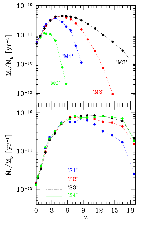
Figure 1: Redshift evolution of the total star formation rate, $\dot{M}_{\star}$, normalized to the total baryonic mass, $M_{b}$, for the field region simulation (upper panel) with four increasing mass resolutions (‘M0’-‘M3’ from left to right). In the lower panel the same quantity is shown for the cluster simulation.

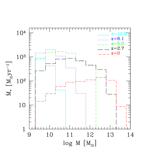
Figure 2: Star formation rate, $\dot{M}_{\star}$, for the ‘M3’ simulation, as a function of the halo mass, $M$. The curves refer to different redshifts: $z=12.8$ (solid line), 8.1 (dotted), 5 (short dashed), 2.7 (long dashed) and 0 (dashed-dotted).

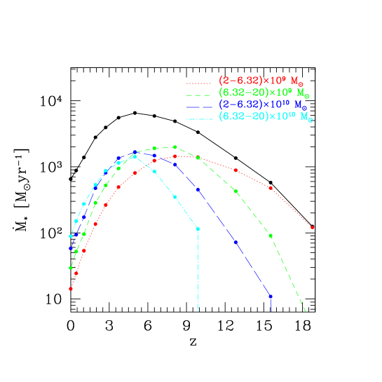
Figure 3: Redshift evolution of the total star formation rate (solid line) and the contribution from haloes with masses in different ranges: $(2-6.32)\times 10^{9}$ M_⊙ (dotted line), $(6.32-20)\times 10^{9}$ M_⊙ (dashed line), $(2-6.32)\times 10^{10}$ M_⊙ (long dashed line) and $(6.32-20)\times 10^{10}$ M_⊙ (dashed-dotted line).

We now use our series of simulations run to check for convergence. In Fig. 1 the total star formation rate, $\dot{M}_{\star}$, normalized to the total baryonic mass, $M_{b}$, is shown as a function of redshift for the field region simulations (upper panel). The ‘M2’ simulation converges to ‘M3’ at $z_{conv}\sim 5.5$, while the ‘M0’ simulation converges to higher resolution results only at $z_{conv}\sim 0$. The lower panel of Fig. 1 shows a similar comparison for the cluster simulations. In comparison to the field region, convergence is reached at earlier times. This is due to the fact that structure growth is accelerated in the proto-cluster region so that its star formation becomes dominated by relatively massive galaxies much earlier than in the field.

Thus, the ‘S2’ and ‘S1’ simulations converge to ‘S3’ already at $z_{conv}\sim 9$ and $z_{conv}\sim 8$, respectively. Comparing the ‘S3’ and the ‘S4’ simulations we conclude that the ‘S3’, which has a mass resolution of $M_{p}=2.4\times 10^{8}h^{-1}$ M_⊙, somewhat lower than ‘M3’, already accounts for all significant star formation. A simulation of the field region with mass resolution comparable to ‘S4’ is not available. We therefore estimate the redshift after which the ‘M3’ run accounts for all star formation by deriving the contribution to the total star formation from objects with masses in different ranges.

In Fig. 2 we plot $\dot{M}_{\star}$ as a function of the halo mass, $M$ at different redshift. The bins are 0.5 wide, in units of log $M$ and they have been chosen so that the lower limit is equivalent to our mass resolution. Before redshift $\sim 10$ the main contribution comes from the smallest mass objects, but larger and larger objects become important as the redshift decreases. This can be seen more clearly in Fig. 3 where the redshift evolution of the total star formation rate is plotted (solid line) together with the contribution from haloes with masses in different ranges. As expected, at the higher redshifts the major contribution comes from objects with mass of few $10^{9}$ M_⊙. At $z\sim 11$ their contribution drops below half of the total. We have plotted the contribution of haloes with mass up to $\sim 10^{11}$ M_⊙, as more massive objects are important only at $z<5$, and thus are not relevant for our study. From this analysis we can conclude that the ‘M3’ simulation accounts for most star formation at $z\lower 2.15277pt\hbox{$\;\buildrel<\over{\sim}\;$}11$.

3 Radiative Transfer

To follow the propagation of ionizing radiation produced by the sources through the given IGM density distribution, we use the Monte Carlo (MC) radiative transfer code CRASH (Cosmological RAdiative transfer Scheme for Hydrodynamics) described in CFMR. It should be noted that in the present study a wider range of densities is encountered, reaching values of the optical depth of a few hundreds in the highest density regions. For this reason, additional tests, that we do not report here, have been run to check its reliability, finding that it reaches the same accuracy providing a right number of photon packets is emitted (see below). For clarity, we briefly summarize the main features of the numerical scheme relevant to the present study.

In the application of a MC scheme to radiative transfer problems, the radiation intensity is discretized into a representative number of monochromatic photon packets. Then, all the processes involved (e.g. packet emission and absorption) are treated statistically by randomly sampling the appropriate distribution function and solving the time-dependent ionization equation. Differently from CFMR, here we deal with more than one ionizing source. In this case, a better solution of the discretized time-dependent ionization equation is obtained if the time step $\Delta t$ used in their eq. 10 is not treated statistically. Thus, here $\Delta t$ is the time elapsed since a photon packet has gone through the cell for which the equation is being solved. The only inputs needed for the calculation are the gas density field and ionization state, as well as the source positions and emission properties. Then, CRASH provides the final gas ionization state, while the gas density field remains constant throughout the radiative transfer simulation. The above procedure is repeated for each output of the N-body simulation described in the previous Section. The inputs and the CRASH running time, $t_{rt}$, are changed accordingly; in particular, $t_{rt}=t_{out}$, the time between two outputs of the simulation. In the following, we discuss how the above inputs are derived and updated.

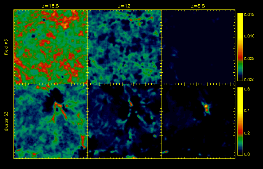
Figure 4: Slices through the simulation boxes. The six panels show the neutral hydrogen number density for the field region (upper panels) and the proto-cluster (lower panels), at redshift, from left to right, $z=16.5,12$ and 8.5. The simulation box of the field region (proto-cluster) has a comoving length of $L\sim 20h^{-1}$ Mpc ($10h^{-1}$ Mpc).

For each output of the N-body simulation, the dark matter density distribution, $n_{dm}$, is tabulated on a mesh using a Triangular Shaped Cloud (TSC) interpolation (Hockney & Eastwood 1981). We discuss the effect of neglecting density variations on sub-grid scales in Section 5. Assuming that the gas distribution follows that of the dark matter, we set the gas density in each grid cell by requiring the adimensional baryon density to be $\Omega_{b}=0.04$. A number $N_{c}=128^{3}$ of cells have been used (see Section 5 for a discussion on this choice). As long as the sources are of stellar type, the presence of helium does not sensibly affect the H reionization process. For this reason, we consider a gas of pure hydrogen. Moreover, a simulation with an H/He gas, although feasible with the updated version of the code CRASH (Maselli, Ferrara & Ciardi 2003), would be extremely time consuming. The other quantities, such as temperature, $T$, and ionization fraction, $x$, are initialized as in CFMR and updated as described in the following paragraphs.

The source positions are obtained directly from the outputs of the N-body simulations, as described in the previous Section. In order to reduce the computational cost of the calculation, we group all sources in a grid cell into a single source placed at the cell center. Mass and luminosity conservation are assured. To further reduce the computational cost of the radiative transfer simulation, each source is modeled with a number of photon packets proportional to its luminosity, i.e. its star formation rate. In practice, this means that we randomly sample the source luminosity distribution function. For the range of densities considered here, we find that a number of photon packets equal to ${\cal N}_{p}=\left[5\times 10^{7}\left(E/10^{60}{\rm erg}\right)\right]$, where $E$ is the total ionizing energy emitted at each output of the simulation, is needed to reach numerical convergence in the volume averaged ionization fraction to within few percent. If we were rather interested, e.g., in resolving the ionization fronts, a much higher number of photons packets would have been required (Maselli, Ferrara & Ciardi 2003). Of the emitted packets, only $f_{esc}{\cal N}_{p}$ will actually be able to escape from the galaxies and break into the IGM. The packets have the same energy, ${\cal E}_{p}=E/{\cal N}_{p}$, but contain a different number of monochromatic photons. We determine $E$ as follows. As ionizing photon production decreases rapidly as stars age, the bulk of the ionizing radiation is produced by newly formed stars. We thus assume that a mass of stars $M_{\star}=t_{out}\times\sum_{i=1}^{n_{s}}\dot{M}_{\star,i}$, is responsible for the all emission, neglecting the contribution from stars formed in previous outputs. This is a good approximation as long as $t_{out}\lower 2.15277pt\hbox{$\;\buildrel>\over{\sim}\;$}10^{7}$ yr, the mean lifetime of an OB star. $\dot{M}_{\star,i}$ is the star formation rate of the i-th galaxy and $n_{s}$ is the number of galaxies at the output under consideration. We derive $E$ integrating over $t_{out}$ the time-dependent SED of a Simple Stellar Population of metal-free stars, with a total mass $M_{\star}$, distributed according to a Salpeter IMF (see Section 2).

Given the above density distribution, source positions and emission properties, we run the code CRASH for the time $t_{out,k}$, corresponding to the output, $k$, under consideration. Before running CRASH for the next output, $k+1$, we update the relevant physical quantities as it follows. Let’s assume that the i-th cell has an ionization fraction $x_{i}$; we thus assign to each particle in the cell, $p_{i}$, the value $x_{i}$. We follow the same procedure for all the cells. At the output $k+1$ the $p_{i}$ particles may have moved into another cell. We thus reconstruct the new distribution of particles, together with their ionization fraction. Then, when we grid the box of the simulation at the $k+1$ output, we assign to each cell an ionization fraction averaged over those of the particles that end up in that cell. Particles flowing in from the external boundaries inherit the properties of the particles in the cell. This procedure is performed for all the quantities relevant to the calculation, with the exception of the gas density, which is updated from the simulations as described above. In this way, we can follow the reionization process in an evolving universe.

Finally, to mimic the presence of an unknown background, photons escaping from a side of the box re-enter from the opposite side. At the early times, when HII regions are still confined around their sources, few photons exit the box. Their number increases rapidly as the regions start to overlap. This is consistent with the expected build up of an ionizing background (e.g. Gnedin 2000).

4 Results

As discussed in the previous Sections, to study the effect of the environment on the reionization process, we have performed the same radiative transfer simulation on a 20 $h^{-1}$ Mpc comoving box positioned in a field region of the universe and on a 10 $h^{-1}$ Mpc comoving box centered on a clustered region. It should be noticed that in the redshift range where the radiative transfer simulations are applied, the cluster has not yet collapsed. The application of the CRASH code in its first version, that does not follow the detailed temperature evolution, is thus appropriate, since less than 1% of the gas is in regions with $T>>10^{4}$ K (see also Mo & White 2002). In the following we present the results of our simulations.

In Fig. 4 we show illustrative slices cut through the simulation boxes. The six panels show the neutral hydrogen number density for the ‘M3’ field region (upper panels) and the ‘S3’ proto-cluster (lower panels), at redshifts, from left to right, $z=16.5,12$ and 8.5. The ionized regions (black) clearly grow differently in the two environments. In the field, high density peaks are uncommon and HII regions easily break into the IGM; in the proto-cluster the density is higher, so ionization is more difficult and recombination is faster. Moreover, many photons are initially needed to ionize the high density gas surrounding the sources, before photons can escape into the low density IGM. As a result, more photons are required to ionize the proto-cluster region; although in the proto-cluster the ionizing photon production per unit mass is higher at high redshift (see Fig. 1), filaments of neutral gas are still present after the field region is almost completely ionized.

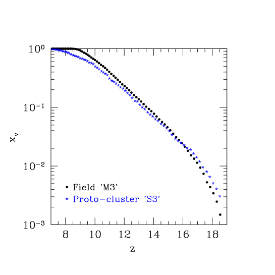
Figure 5: Redshift evolution of the volume averaged ionization fraction, $x_{v}$, for the ‘M3’ field region (filled circles) and ‘S3’ proto-cluster (asterisks).

This is more clearly seen in Fig. 5, where the volume averaged ionization fraction, $x_{v}$, is shown as a function of redshift for ‘M3’ and ‘S3’. This ionization fraction is defined as $x_{v}=\sum_{i}x_{i}V_{i}/V$, where $x_{i}$ and $V_{i}$ are the ionization fraction and volume of the $i$-th cell respectively, and $V$ is the total volume of the box. The evolution proceeds differently in the two regions: initially the ionization fraction are comparable, but the proto-cluster gas ionizes more slowly, for the reasons discussed above. While the ‘M3’ field region already has $x_{v}\sim 0.999$ at $z=8.3$, $x_{v}\sim 0.8$ for the proto-cluster at the same redshift.

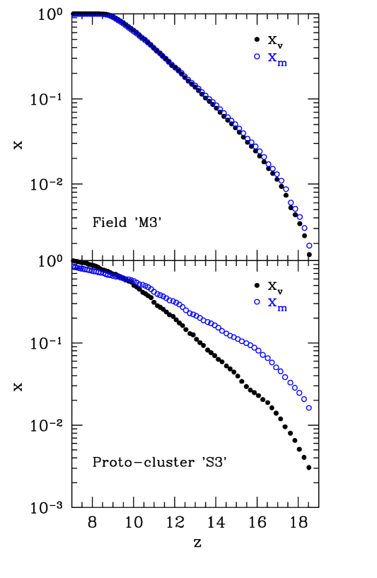
Figure 6: Redshift evolution of ionization fraction for the ‘M3’ field region (upper panel) and the ‘S3’ proto-cluster (lower panel). Volume (filled circles) and mass (open circles) averaged ionization fraction ($x_{v}$ and $x_{m}$, respectively) are shown.

A comparison between volume and mass averaged ionization fractions is useful to understand how the reionization process proceeds. We define the latter quantity as $x_{m}=\sum_{i}x_{i}M_{i}/M$, where $M_{i}$ is the mass in the $i$-th cell and $M$ is the total mass in the box. In Fig. 6 the redshift evolution of $x_{v}$ (filled circles) and $x_{m}$ (open circles) is compared both for the ‘M3’ field region (upper panel) and for the ‘S3’ proto-cluster (lower panel). The most interesting feature of these plots is that, while for the field region $x_{m}$ is always comparable with $x_{v}$, $x_{m}>x_{v}$ initially in the proto-cluster, i.e. at first relatively dense cells are ionized. This because the density immediately surrounding the sources must be ionized, before the photons can break into the IGM. This indicates that the assumption adopted by some authors (e.g. Miralda-Escudé, Haehnelt & Rees 2000), that lower density gas always gets ionized before higher density regions, fails in a cluster environment. The trend reverses at later times, when large, low density regions get ionized and the highest density peaks remain neutral or recombine. Although almost 90% of the proto-cluster volume is ionized by $z\sim 8$, this is true for only $\sim 70\%$ of the mass.

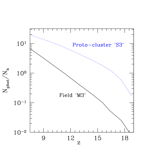
Figure 7: Ratio between the cumulative number of escaping ionizing photons, $N_{phot}$, and the number of baryons, $N_{b}$, as a function of redshift for the ‘M3’ field region (solid line) and the ‘S3’ proto-cluster (dotted line).

Some approaches to the study of the reionization process adopt the one-photon-per-baryon approximation. This is valid only in cases when recombination can be safely neglected. An estimate of the photon budget required to ionize the IGM in a more realistic case is shown in Fig. 7, where the ratio between the cumulative number of escaping ionizing photons, $N_{phot}$, and the number of baryons, $N_{b}$, is plotted as a function of redshift for the ‘M3’ field region (solid line) and the ‘S3’ proto-cluster (dotted line). High density peaks, where star formation preferentially takes place, are more abundant in the proto-cluster, so photon production is higher there than in the field region, at least up to $z\sim 11$. At $z\sim 8$, when $x_{v}=0.999$, about 5 photons per baryon have been produced in the field region. However, the $\sim 15$ photons per baryon produced in the proto-cluster are not enough to reionize it completely for the reasons discussed above.

5 Discussion

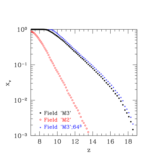
Figure 8: Redshift evolution of volume averaged ionization fraction, $x_{v}$, for the ‘M3’ (filled circles) and the ‘M2’ (open circles) field region and for the ‘M3’ field region with $N_{c}=64^{3}$ (asterisks).

In the following we will discuss the convergence of our simulations with respect to mass and grid resolution. To assess the impact of mass resolution on our results, we have run a reionization simulation on the ‘M2’ field region. The redshift evolution of $x_{v}$ is shown in Fig. 8 as open circles. The ‘M2’ and ‘M3’ curves converge only at $z<7$. The difference observed at higher redshift is due to the mass resolution, which, for the ‘M2’ simulation, is not enough to resolve the objects that give the main contribution to the ionizing radiation, as is evident from the upper panel of Fig. 1. From Figs. 2-3 we are confident that the ‘M3’ simulation has the appropriate resolution to account for the bulk of ionizing photon production, at least after $z\sim 11$. It should be noticed that the formation and evolution of objects with $M<10^{9}$ M_⊙ may be affected by feedback effects, that inhibit their star formation (e.g. Haiman, Rees & Loeb 1997; Omukai & Nishi 1999; Mac Low & Ferrara 1999; Barkana & Loeb 1999; Ciardi et al. 2000; Glover & Brand 2000; Nishi & Tashiro 2000; Kitayama et al. 2001; Glover & Brand 2002; Benson et al. 2002). Thus, these smaller mass structures may well play a minor role in the reionization process.

To assess the impact of grid resolution we have rerun our radiative transfer simulations with $N_{c}=64^{3}$. The resulting evolution of $x_{v}$ is shown in Fig. 8 by asterisks. From this figure it is evident that the grid resolution does not greatly affect the final results; the value of $x_{v}$ never differs in the two runs by more than 10 or $20\%$, although the case with $N_{c}=64^{3}$ produces slightly higher values. $N_{c}>128^{3}$ is not allowed by the mass resolution of our N-body simulation, as sampling fluctuations in the density field then become large.

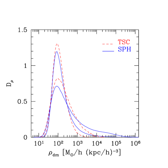
Figure 9: Distribution of DM densities at the positions of the DM particles, for a 32-particle SPH smoothing kernel (solid line) and the TSC interpolation scheme (dashed). The upper two curves show the distributions for $z=10$, the lower ones for $z=6$. $D_{p}$ gives the relative number of particles per $\log\rho$ interval.

As mentioned above, small mass objects, although negligible for ionizing photon production, are important because small-scale clumping can enhance recombination. Simulations which do not include such objects may underestimate the actual number of ionizing photons needed to reionize the IGM. To mimic clumping on unresolved scales, a so called clumping factor, $C$, is often introduced. It is defined as $C=<n^{2}>/<n>^{2}$, where $n$ is the density. The TSC technique used to derive our density distributions will lead us to underestimate the clumping factor. The TSC interpolation has the advantage of producing smoothed density values at the positions of the grid cells, as required for the radiative transfer computation. However, this technique is not adaptive, like an SPH kernel for example, and density variations on sub-grid scales are smoothed out, reducing the contrast of the DM density peaks where our sources are positioned. This results in an underestimate of the recombination rate and thus faster reionization. In order to address the importance of this effect we have measured densities at the particle positions using both the TSC interpolation and a 32-particle SPH smoothing kernel. The result of this comparison for ‘M3’ at redshifts $z=10$ and $z=6$ is shown in Fig. 9. The overall agreement for low and intermediate densities is reasonable, but the smoothing of the TSC scheme is clearly visible at the high densities. This is especially true at $z=6$. An estimate of the error introduced can be quantified by the ratio of the total recombination rate derived with the two different schemes, $r_{SPH}/r_{TSC}$. This ratio is equal to 6.24 (20.87) at $z=10$ (6), suggesting that we are substantially underestimating the recombination rate in the high density regions surrounding the sources. We are interested primarily in the higher redshifts, where agreement is somewhat better. Since almost all the high density regions where the above corrections are important host sources, the error in the recombination rate can be considered part of the uncertainty on our adopted escape fraction (see below). Moreover, the effect of clumping is alleviated by photoevaporation, which tends to weaken the effect of gas on unresolved scales as ionization precedes (Shapiro et al. 2003).

The number of available ionizing photons depends on the choice of the stellar spectrum, IMF and escape fraction. As the first stars form out of gas of primordial composition, they are thought to be very massive, resulting in a higher ionizing photon emission, when compared with higher metallicity stars (e.g. Larson 1998). For example, Schneider et al. (2002) propose that enrichment is needed to permit further fragmentation into stars with significantly lower masses, inducing a transition from a top-heavy to a more conventional IMF. The debate on the metallicity and the IMF of the first stars is still very lively and many authors argue that metal-free stars are distributed according to a top-heavy IMF. On the other hand, Christlieb et al. (2002) recently discovered a low mass star with metallicity only $3\times 10^{-6}$ that of the Sun. To be conservative, in this paper we have assumed metal-free stars with a Salpeter IMF.

Even more uncertain is the value of the escape fraction. Values derived in previous work vary from 0 to 60% (see e.g. Wood & Loeb 1999; Ricotti & Shull 2000; Ciardi, Bianchi & Ferrara 2002 for theoretical work and e.g. Leitherer et al. 1995; Hurwitz et al. 1997; Bland-Hawthorn & Maloney 1999; Steidel, Pettini & Adelberger 2001 for observations), according to the galaxy mass, redshift and density distribution. Given these uncertainties and the impossibility of accurately modeling this parameter for every galaxy (see e.g. Ciardi, Bianchi & Ferrara 2002 for a discussion), we regard $f_{esc}=5\%$ as a constant, reference value. It should be noticed that, as the resolution of the radiative transfer calculation is equivalent to the dimension of a single grid cell (which is always larger than the dimension of the sources), $f_{esc}$ is actually an “effective” escape fraction, i.e. it includes both the contribution to the absorption of the interstellar medium in the emitting object (“real” escape fraction) and the one of the IGM in the same cell as the object.

Although it is not possible to disentangle different choices for the source emission properties from clumping on small scales, their expected global effect can be estimated introducing the parameter ${\cal A}=C_{n}^{-1}(f_{esc}/0.05)(N_{\gamma}/1\times 10^{61}{\rm M}_{\odot}^{-1})$, where $C_{n}$ is the clumping factor normalized to the value of our simulations (e.g. $C_{n}=2$ means that the clumping factor is twice that of the simulations) and $N_{\gamma}$ is the total number of ionizing photons per unit solar mass of formed stars produced by the adopted spectrum and IMF. $N_{\gamma}$ is normalized to a Salpeter IMF and a spectrum typical of metal-free stars (CFMR). From a “back of the envelope” calculation, we conclude that if ${\cal A}=10$, the $\sim 5$ photons per baryon required to reionize the IGM are already available at $z\sim 13$, while if ${\cal A}=0.1$ the above condition is never reached. As the most recent observations of high redshift quasars (Becker et al. 2001; Djorgovski et al. 2001; Pentericci et al. 2002) suggest that the universe was already ionized at $z\sim 6.3$, the lowest value of ${\cal A}$ consistent with this constraint is $\sim 0.7$. A lower value of ${\cal A}$ would require additional sources of ionizing photons to produce the observed ionization level. In a forthcoming paper we will discuss the possible contribution to ionizing radiation from a primordial population of quasars (see also Wyithe & Loeb 2002). In a recent paper Ricotti (2002) has suggested that a possible contribution to ionizing photons could also come from globular clusters. Given our conservative assumptions on the value of the escape fraction and the IMF, a higher value of the clumping factor would also be compatible with a reionization driven by primordial stellar sources.

Recent results from the WMAP satellite require a mean optical depth to Thomson scattering $\tau_{e}\sim 0.17$, suggesting that reionization must have begun at relatively high redshift (e.g. Kogut et al. 2003; Spergel et al. 2003). Reconciling an early reionization with observations of the Gunn-Peterson effect in $z>6$ quasars, which imply a volume-averaged neutral fraction above $10^{-3}$ at $z\sim 6$, may be challenging. In Ciardi, Ferrara & White (2003) we run additional simulations and discuss our model in view of these new data.

6 Conclusions

We have studied the IGM reionization process in a full cosmological context with structure evolution and a realistic galaxy population. We have used a combination of high-resolution N-body simulations (to describe the dark component of matter), a semi-analytic model of galaxy formation (to track the gas evolution) and the Monte Carlo radiative transfer code CRASH (to follow the propagation of ionizing photons into the IGM; CFMR). The process has been followed in the largest volume ever used for this kind of study, with a comoving length of $L\sim 20h^{-1}$ Mpc, a mass resolution of $\sim 10^{8}$ M_⊙ and tree from periodic boundary conditions. This allows us to resolve the primary objects responsible for the production of ionizing radiation and, at the same time, to simulate a region of the universe with “mean” properties. To study the effect of environment on the reionization process, we have performed the same radiative transfer simulation on a $10h^{-1}$ Mpc comoving box, centered on a proto-cluster region. The main results discussed in this paper can be summarized as follows.

(1) Our field region of the universe gets reionized by the simulated galaxy population at a redshift $z_{ion}\sim 8$, while the proto-cluster, although it produces a higher number of ionizing photons, gets ionized later. This is due to the fact that high density gas, which is more common in the proto-cluster, is more difficult to ionize and recombines much faster.

(2) While for the field region $\sim 5$ photons per baryon are enough to produce $x_{v}=0.999$ at $z\sim 8$, the $\sim 15$ photons per baryon produced by this time in the proto-cluster are not enough to reionize it.

(3) For the same reason, while for the field region the mass and volume averaged ionization fractions, $x_{m}$ and $x_{v}$ respectively, are always comparable, $x_{m}$ substantially exceeds $x_{v}$ for the proto-cluster, at high redshifts. This is because the high density regions surrounding the sources have to be ionized first, before the photons can break out into the low density IGM.

(4) The primordial stellar sources considered in this study give a value of the reionization epoch consistent with observation, without invoking the presence of additional sources of ionization. Our conservative assumptions on the value of the escape fraction and the IMF can accommodate the additional clumping which remains unresolved in our scheme.

(5) The mass resolution of the simulations can deeply affect the final results. Objects with total masses of $M\sim 10^{9}$ M_⊙ or less must be resolved to account for the bulk of the star formation.

References

- [1] Abel, T., Norman, M. L. & Madau, P. 1999, ApJ, 523, 66
- [2] Abel, T. & Wandelt, B. D. 2002, MNRAS, 330, L53
- [3] Barkana, R. & Loeb, A. 1999, ApJ, 523, 54
- [4] Baugh, C. M., Cole, S., Frenk, C. S., Lacey, C. G., 1998, ApJ, 498, 504
- [5] Becker, R. H. et al. 2001, AJ, 122, 2850
- [6] Benson, A. J., Baugh, C. M., Cole, S., Frenk, C. S. & Lacey, C. G. 2000, MNRAS, 316, 107
- [7] Benson, A. J., Lacey, C. G., Baugh, C. M., Cole, S. & Frenk, C. S. 2002, MNRAS, 333, 156
- [8] Bland-Hawthorn, J. & Maloney, P. R. 1999, ApJ, 510, 33
- [9] Blanton, M., Cen, R., Ostriker, J. P. & Strauss, M. 1999, ApJ, 522, 590
- [10] Cen, R. 2002, ApJS, 141, 211
- [11] Cen, R. & Ostriker, J. P. 1993, ApJ, 417, 415
- [12] Cen, R. & Ostriker, J. P. 2000, ApJ, 538, 83
- [13] Chiu, W. A. & Ostriker, J. P. 2000, ApJ, 534, 507
- [14] Ciardi, B. 2002, in ”The Evolution of Galaxies. II. Basic Building Blocks” proceedings, Ile de la Reunion, France, October 16-21 2001; eds. M. Sauvage, G. Stazinska & D. Schaerer; Kluwer Academic Publishers; pp. 515-518
- [15] Ciardi, B., Bianchi, S. & Ferrara, A. 2002, MNRAS, 331, 463
- [16] Ciardi, B., Ferrara, A., Governato, F. & Jenkins, A. 2000, MNRAS, 314, 611
- [17] Ciardi, B., Ferrara, A., Marri, S. & Raimondo, G. 2001, MNRAS, 324, 381 (CFMR)
- [18] Ciardi, B., Ferrara, A. & White, S. D. M. 2003, astro-ph/0302451
- [19] Cojazzi, P., Bressan, P., Lucchin, F., Pantano, O. & Chavez, M. 2000, MNRAS, 315, 51
- [20] Cole, S., Lacey, C. G., Baugh, C. M. & Frenk, C. S. 2000, MNRAS, 319, 168
- [21] Cowie, L. L., & Songaila, A. 1998, Nature, 344, 44
- [22] Christlieb, N. et al. 2002, Nature, 419, 904
- [23] Devriendt, J. E. S., Sethi, S. K., Guiderdoni, B. & Nath, B. B. 1998, MNRAS, 298, 708
- [24] Diaferio, A. et al. 2001, MNRAS, 323, 999
- [25] Djorgovski, S. G., Castro, S., Stern, D. & Mahabal, A. A. 2001, ApJ, 560, L5
- [26] Ellison, S. L., Songaila, A., Schaye, J. & Pettini, M. 2000, AJ, 120, 1175
- [27] Fan, X. et al. 2000, AJ, 120, 1167
- [28] Fan, X. et al. 2001, AJ, 122, 2833
- [29] Glover, S. C. O. & Brand, P. W. J. L. 2000, MNRAS, 321, 385
- [30] Glover, S. C. O. & Brand, P. W. J. L. 2002, astro-ph/0205308
- [31] Gnedin, N. Y. 2000, ApJ, 535, 530
- [32] Gnedin, N. Y. & Abel, T. 2001, NewA, 6, 437
- [33] Gnedin, N. Y. & Ostriker, J. P. 1997, ApJ, 486, 581
- [34] Gunn, J.E. & Peterson, B.A. 1965, ApJ, 142, 1633
- [35] Haiman, Z. & Loeb, A. 1997, ApJ, 483, 21
- [36] Haiman, Z., Rees, M. J. & Loeb, A. 1997, ApJ, 476, 458
- [37] Heyl, J. S., Cole, S., Frenk, C. S. & Navarro, J. F. 1995, MNRAS, 274, 755
- [38] Hockney, R. W. & Eastwood, J. W. 1981, in ”Computer Simulations Using Particles”; New York: McGrow-Hill
- [39] Hurwitz, M., Jelinsky, P. & Dixon, W. V. 1997, ApJ, 481, L31
- [40] Katz, N., Hernquist, L.& Weinberg, D. H. 1999, ApJ, 523, 463
- [41] Katz, N., Weinberg, D. H.& Hernquist, L. 1996, ApJS, 105, 19
- [42] Kauffmann, G., Colberg, J. M., Diaferio, A. & White, S. D. M. 1999, MNRAS, 303, 188
- [43] Kauffmann, G., Nusser, A. & Steinmetz, M. 1997, ApJ, 286, 795
- [44] Kauffmann, G., White, S. D. M. & Guiderdoni, B. 1993, MNRAS, 264, 201
- [45] Kitayama, T., Susa, H., Umemura, M. & Ikeuchi, S. 2001, MNRAS, 326, 1353
- [46] Kogut, A. et al. 2003, astro-ph/0302213
- [47] Lacey, C., Guiderdoni, B., Rocca-Volmerange, B. & Silk, J. 1993, ApJ, 402, L15
- [48] Larson, R. B. 1998, MNRAS, 301, 569
- [49] Leitherer, C. et al. 1999, ApJS, 123, 3
- [50] Mac Low, M.-M. & Ferrara, A. 1999, ApJ, 513, 142
- [51] Madau, P., Ferrara, A. & Rees, M. J. 2001, ApJ, 555, 92
- [52] Madau, P., Haardt, F. & Rees, M. J. 1999, ApJ, 514, 648
- [53] Maselli, A., Ferrara, A. & Ciardi, B. 2003, in prep.
- [54] Miralda-Escudé, J., Haehnelt, M. & Rees, M. R. 2000, ApJ, 530, 1
- [55] Mo, H. J., Mao, S. & White, S. D. M. 1998, MNRAS, 295, 319
- [56] Mo, H. J. & White, S. D. M. 2002, MNRAS, 336, 112
- [57] Nishi, R. & Tashiro, M. 2000, ApJ, 537, 50
- [58] Omukai, K. & Nishi, R. 1999, ApJ, 518, 64
- [59] Pearce, F. R. et al. 2001, MNRAS, 326, 649
- [60] Pentericci et al. 2002, ApJ, 123, 2151
- [61] Razoumov, A. O., Norman, M. L., Abel, T. & Scott, D. 2002, ApJ, 572, 695
- [62] Razoumov, A. & Scott, D. 1999, MNRAS, 309, 287
- [63] Ricotti, M. 2002, astro-ph/0208352
- [64] Ricotti, M. & Shull, J. M. 2000, ApJ, 542, 548
- [65] Schaye, J., Rauch, M., Sargent, W. L. W. & Kim, T. 2000, ApJ, 541, L1
- [66] Schneider, R., Ferrara, A., Natarajan, P. & Omukai, K. 2002, ApJ, 571, 30
- [67] Shapiro, P. R., Iliev, I. T., Raga, A. C. & Martel, H. 2003, astro-ph/0302339
- [68] Somerville, R. S., Primack, J. R. & Faber, S. M. 2001, MNRAS, 320, 504
- [69] Spergel, D.N. et al. 2003, astro-ph/0302207
- [70] Springel, V., White, S. D. M., Tormen, G. & Kauffmann, G. 2001, MNRAS, 328, 726 (SWTK)
- [71] Springel, V., Yoshida, N. & White, S. D. M. 2001, NewA, 6, 79
- [72] Steidel, C. C., Pettini, M. & Adelberger, K. L. 2001, ApJ, 546, 665
- [73] Umemura, M., Nakamoto, T. & Susa, H. 1999, in Numerical Astrophysics, eds.Miyama et al. (Kluwer: Dordrecht), p.43
- [74] Valageas, P. & Silk, J. 1999, A&A, 347, 1
- [75] Weinberg, D. H., Hernquist, L.& Katz, N. 2002, ApJ, 571, 15
- [76] Wyithe, J. S. B. & Loeb, A. 2002, astro-ph/0209056
- [77] Wood, K. & Loeb, A. 1999, AAS, 195, 1309
- [78] Yoshida, N., Sheth, R. K. & Diaferio, A. 2001, MNRAS, 328, 669