Evolution of the Mass Function of Dark Matter Haloes

Abstract

We use a high resolution $\Lambda$CDM numerical simulation to calculate the mass function of dark matter haloes down to the scale of dwarf galaxies, back to a redshift of fifteen, in a 50 $h^{-1}$Mpc volume containing 80 million particles. Our low redshift results allow us to probe low $\sigma$ density fluctuations significantly beyond the range of previous cosmological simulations. The Sheth and Tormen mass function provides an excellent match to all of our data except for redshifts of ten and higher, where it overpredicts halo numbers increasingly with redshift, reaching roughly 50 percent for the $10^{10}-10^{11}{\rm{M}}_{\odot}$ haloes sampled at redshift 15. Our results confirm previous findings that the simulated halo mass function can be described solely by the variance of the mass distribution, and thus has no explicit redshift dependence. We provide an empirical fit to our data that corrects for the overprediction of extremely rare objects by the Sheth and Tormen mass function. This overprediction has implications for studies that use the number densities of similarly rare objects as cosmological probes. For example, the number density of high redshift (z $\simeq$ 6) QSOs, which are thought to be hosted by haloes at 5$\sigma$ peaks in the fluctuation field, are likely to be overpredicted by at least a factor of 50$\%$. We test the sensitivity of our results to force accuracy, starting redshift, and halo finding algorithm.

1 Introduction

Cold dark matter models with a cosmological constant ($\Lambda$CDM) are successful in explaining a wide array of kinematic and structural properties of the observed universe. A critical test of the $\Lambda$CDM model is how well it predicts the abundance of dark matter haloes, which serve as hosts for observable clusters, groups, and galaxies. Simulations that resolve haloes out to high redshift can be used to model the evolution of the numbers of observable high redshift objects, their progenitors, and their evolved descendants. Lyman break galaxies, for example, observed at redshifts out to z $\simeq$ 4 (e.g. Steidel et al. 1996) are likely progenitors of groups or clusters (Governato et al. 1998; Governato et al. 2001), and we are able to model their numbers over their entire observable lifespan. Many objects, however, lie outside the realm that can presently be simulated because their number densities, masses, or redshifts are too extreme. For example, to model a reasonably sized sample of the hosts of the highest redshift (z $\simeq$ 6) quasi-stellar objects (QSOs), whose number density has been measured by the Sloan Digital Sky Survey (Fan et al. 2001), would require a simulation with volume roughly as large as the observable universe with (so far) prohibitively high particle numbers. Simulations of adequate resolution and volume could be used, in principle, to estimate the host masses of such rare QSOs, or to estimate cosmological parameters after assuming host masses, by matching predicted and observed number densities. However, with much less computational effort, by modeling smaller cosmological volumes at higher redshift, we are able to test analytic mass functions in the same regime of rare density enhancements. Generally, rare density peaks correspond to high values of M/M_∗, where M_∗ is the ‘characteristic’ mass of a typical collapsing halo at that epoch (to be discussed later). By modeling haloes over a wide range of M/M_∗, we can constrain analytic mass functions for ranges of redshift and mass that have not yet been simulated. This is possible because analytic mass functions are generally derived from assumptions of how linear density fluctuations lead to halo collapse, and thereby have no explicit redshift dependence. High redshift QSO hosts, galaxy progenitors, and perhaps even the first generation of stars are all examples of high $M/M_{*}$ objects whose mass functions can presently only be calculated analytically.

Press & Schechter (P-S, 1974) developed an analytical framework that predicts the number and formation epoch of dark matter haloes. In P-S theory, as the universe evolves, linear density fluctuations grow gravitationally until they reach a critical spherical overdensity, at which time non-linear gravitational collapse is assumed to occur. Cosmological numerical simulations have shown the P-S framework to be approximately correct, but P-S theory consistently underpredicts the number of high mass haloes and overestimates the number of haloes less than about $M_{*}$ (e.g. Efstathiou et al. 1988; Gross et al. 1998; Governato et al. 1999; Jenkins et al. 2001; White 2002) even when merging of dark matter haloes is included in predictions (Bond et al. 1991; Bower 1991; Lacey & Cole 1993; Gardner 2001), though the high mass end fits well if the finite size of haloes is taken into account (Yano, Nagashima, & Gouda 1996; Nagashima 2001). Ellipsoidal halo collapse models (e.g. Monaco 1997ab; Lee & Shandarin 1998; Sheth, Mo, & Tormen 2001) yield much more robust predictions than the conventional spherical collapse models, and are in excellent agreement with empirical fits by Sheth & Tormen (1999). Monaco et al. (2001), using the semi-analytic code PINOCCHIO, which uses a perturbative approach, show that the dark matter halo distribution can be accurately predicted at much lower computational cost, on a point-by-point basis, from a numerical realization of an initial density field. Jenkins et al. (2001) utilize a large set of simulations of a range of volumes and cosmologies (Jenkins et al. 1998; Governato et al. 1999; Evrard et al. 2002) to test the Sheth & Tormen (S-T) mass function over more than four orders of magnitude in mass, and out to a redshift of 5, finding good agreement with the S-T function down to their resolution limit of $\simeq 3\times 10^{11}{\rm{M}}_{\odot}$, except for an overprediction by the S-T function for haloes at rare density enhancements. In this study, we probe previously untested regimes of the mass function by simulating a volume that resolves haloes down to the scale of $10^{10}{\rm{M}}_{\odot}$ dwarfs, in a cosmological environment, allowing us to sample the mass function back to z$\simeq$15. Our paper is outlined as follows: in section 2, we describe our simulations and numerical techniques; in section 3, we review the analytic theory; then we discuss our results and compare with previous work in section 4; we conclude with a discussion of the implications of our work.

2 The simulations

Our cosmology is the presently favored $\Lambda$CDM with $\Lambda=0.7$ and $\Omega_{m}=0.3$. We use the parallel tree gravity solver PKDGRAV (Stadel 2001) to simulate $81\times 10^{6}$ (432³) dark matter particles from a starting redshift, z₀, of 69. We then resimulate the same volume but with z${}_{0}=$139, and evolve this volume to z$=$7; which allows us to consider results at higher redshift than with the z${}_{0}=$69 run. In order to simulate the highest possible mass resolution, we employ a volume of 50 $h^{-1}$Mpc on a side. Our particle mass is $1.3\times 10^{8}h^{-1}{\rm{M}}_{\odot}$ allowing us to resolve haloes down to less than $10^{10}h^{-1}{\rm{M}}_{\odot}$ with 75 particles. Our force resolution is 5 $h^{-1}$kpc. We use a cell opening angle of $\Theta<$ 0.8 at low redshift, and $\Theta<$ 0.7 at z $>$ 2. In section 4.2, we discuss tests that confirm that our choices of initial redshift, softening, and high redshift opening angle are adequate (see Table 1). We use a “multistepping” approach, where particles in the highest density regions undergo 16,000 timesteps. Timesteps were constrained to $\delta t<0.2\sqrt{\epsilon/a}$, where $\epsilon$ is the softening length and $a$ is the magnitude of the acceleration of a given particle. We normalize the density power spectrum of our initial conditions such that $\sigma_{8}$, the rms density fluctuation of spheres of 8 $h^{-1}$Mpc extrapolated to redshift of zero is 1.0, consistent with both the cluster abundance (see e.g. Eke, Cole, & Frenk 1996 and references therein) and the COBE normalization (e.g. Ratra et al. 1997). To set our initial conditions, we use the Bardeen et al. (1986) transfer function with $\gamma=\Omega_{m0}h$, where $h$ is the hubble constant in units of 100 $kms^{-1}Mpc{-1}$.

2.1 Halo Identification

In order to identify haloes in our simulation, we use both the friends-of-friends (FOF) algorithm (Davis et al. 1985), and the spherical overdensity (SO) algorithm (Lacey & Cole 1994). The FOF halo finder uses a “linking length”, ll, to link together all neighboring particles with spacing closer than ll as members of a halo. SO identifies haloes by identifying spherical regions with the expected spherical overdensities of virialized haloes. For our SO haloes, we first use SKID (Stadel 2001) to identify all bound haloes, including those that are subhaloes within larger haloes. Next, we grow a sphere outward from each SKID center until it just contains the virialized overdensity. Finally, we iterate by growing spheres outward from all neighboring SKID haloes until we have identified the center of mass for each SO halo. For our SO criterion, we use the virial overdensity predicted by the spherical collapse tophat model of Eke, Cole, & Frenk (1996). In a $\Lambda$CDM universe, the virial overdensity, in units of critical density, declines from an asymptotic value of 178 as cosmic time increases and $\Omega_{m}$ drops below 1; for redshift of zero, the $\Lambda$CDM overdensity $\Delta_{vir}$ is 100 (Kitayama & Suto 1996). We exclude haloes that contain less than 64 particles, which is conservative, as it is more than the estimated 20 or 30 particles needed for a robust halo identification based on resolution tests (Jenkins et al. 2001; Governato et al. 1999).

We utilize the FOF algorithm for the bulk of our analyses since it is reasonably robust and computationally efficient. Our FOF ll choice is 0.2 for all redshifts (except when matching $ll$ from previous studies); this approach has been shown to be sound for a range of cosmologies by Jenkins et al. (2001), although the evolution of $\Delta_{vir}$ in the spherical collapse tophat model implies that $ll$ should range from $ll=$0.164 at z$=$0 to $ll=$0.2 at high redshift in $\Lambda$CDM cosmology (Lacey & Cole 1994; Eke, Cole, & Frenk 1996; Jenkins et al. 2001). To test the sensitivity of the mass function to halo selection criteria, we apply both FOF $ll=$0.164 and SO to our data at various redshifts, discussed in section 4.1.

3 Analytic Theory

Analytic P-S formalism yields the following (See Jenkins et al. 2001, whose notation we adopt in this section, and references therein for further discussion, which we summarize here):

$$f(\sigma;{\rm P{\rm-}S})=\sqrt{2\over\pi}{\delta_{c}\over\sigma}\exp\bigg{[}-{\delta_{c}^{2}\over 2\sigma^{2}}\bigg{]},$$ (1)

where $\delta_{c}$ is the threshold spherical linear overdensity above which a region will collapse. $\delta_{c}$ depends only weakly on the cosmological parameters and redshift (e.g. More, Heavens, & Peacock 1986; Jenkins et al. 2001), and $\delta_{c}=1.686$ for $\Omega_{0}=1$. In our analysis, we assume that $\delta_{c}=1.686$ at all redshifts. $\sigma^{2}(M,z)$ is the variance of the linear density field, smoothed with a spherical top-hat filter enclosing mass $M$, and is calculated from the linear density power spectrum $P(k)$, extrapolated to $z=0$:

$$\sigma^{2}(M,z)={b^{2}(z)\over 2\pi^{2}}\int_{0}^{\infty}k^{2}P(k)W^{2}(k;M){\rm d}k,$$ (2)

where $W(k;M)$ is the Fourier-space top-hat filter, and ${\it b(z)}$ is the growth factor of linear perturbations normalized to unity at z$=$0 (Peeble 1993). In the P-S formalism, all mass is contained in haloes:

$$\int_{-\infty}^{\infty}f(\sigma;{\rm P{\rm-}S}){\rm d}\ln\sigma^{-1}=1.$$ (3)

The mass function $f(\sigma,z)$ can be related to the number density, $n(M,z)$, of haloes with mass less than $M$:

$$f(\sigma,z)\equiv\frac{M}{\rho_{0}(z)}{{\rm d}n(M,z)\over{\rm d}\ln\sigma^{-1}},$$ (4)

where $\rho_{0}(z)$ is the mean density of the universe at that time.

The S-T model is a modification to the P-S model based on empirical fits to simulations (Sheth & Tormen 1999), has been shown to reproduce simulation results substantially better than P-S (e.g. Jenkins et al. 2001; White 2002), and is theoretically justified in that it matches P-S formalism derived with ellipsoidal halo collapse models (Sheth, Mo, & Tormen 2001):

$$f(\sigma;{\rm S{\rm-}T})=A\sqrt{{2a\over\pi}}\bigg{[}1+\big{(}{\sigma^{2}\over a\delta_{c}^{2}}\big{)}^{p}\bigg{]}{\delta_{c}\over\sigma}\exp\bigg{[}-{a\delta_{c}^{2}\over 2\sigma^{2}}\bigg{]},$$ (5)

where A=0.3222, $a=0.707$ and $p=0.3$. Jenkins et al. (2001) offer an empirical fit using high resolution simulations of a range of cosmologies. Their fit is constructed in the $f-\ln(\sigma^{-1})$ plane, which has the advantage of being invariant with redshift:

$$\phantom{xxxxxxx}f(\ln\sigma^{-1})=0.315\;\exp\big{[}-|\ln\sigma^{-1}+0.61|^{3.8}\big{]}.$$ (6)

The Jenkins et al. function adjusts for an overprediction by the S-T function for the rare objects at large $\ln\sigma^{-1}$, and is calibrated for the range $-1.2\leq\ln\sigma^{-1}\leq 1.05$, which corresponds to masses down to approximately 3$\times 10^{11}h^{-1}{\rm{M}}_{\odot}$ at present epoch, and includes haloes out to z$=$5, with FOF fixed at $ll=$0.2.

In each of these analytic functions, virialized haloes have a characteristic mass, $M_{*}$(z):

$$\sigma(M_{*}(z))=\delta_{c},$$ (7)

and $\sigma(M,z)=\sigma(M,z=0)b(z)$. ${\it b(z)}$ evolves as $(1+z)^{-1}$ in an $\Omega_{0}=1$ universe, and more slowly in a $\Lambda$CDM universe. $\sigma(M)$ decreases slowly with increasing mass, which leads to the steep redshift dependence of $M_{*}$(z), shown in Fig. 1 for the $\Lambda$CDM universe, and results in a broad mass spectrum of collapsed objects. An important test of analytic mass functions is the accuracy of their predictions at high values of $M/M_{*}$ and $z$. At low redshift, high $M/M_{*}$ haloes would have unrealistically large masses, but at high redshift the steep evolution of $M_{*}$ puts high $M/M_{*}$ objects well into the realm of simulations. Furthermore, the evolution of halo masses that correspond to high $\sigma$ density enhancements means that rare haloes are most easily simulated at high redshift (Fig. 1). Our simulations model the mass function of haloes lying at up to 4$\sigma$ density fluctuations.

Figure 1: The curves correspond to the halo mass of $n\sigma$ fluctuations in the density field, given by $\sigma(M,z)=\delta_{c}/n$, with $n=$1, 2, 3, 4, and 5, from bottom to top. The characteristic mass, $M_{*}$, given by $\sigma(M_{*}(z))=\delta_{c}$, is the 1$\sigma$ curve. The area between the long dashed lines is sampled with poisson errors of less than 20$\%$ in our data.

4 Evolution of the Mass Function

In Fig. 2, we compare the analytic version of the P-S, the S-T, and the Jenkins et al. mass function with our simulation results at several redshifts. The S-T function provides the best fit to our simulation with excellent agreement at all masses and redshifts except for our highest redshift outputs. The P-S function overpredicts substantially everywhere except at the low and high mass extremes. And the Jenkins et al. mass function fits much of our data well at z$=$0, but diverges from our simulation results once well below the limit of its empirical fit of $\ln\sigma^{-1}=-1.2$, which corresponds to $\simeq 4\times 10^{11}h^{-1}{\rm{M}}_{\odot}$ with $\sigma_{8}=1.0$. Note that $\sigma(M,z)$ is sensitive to $\sigma_{8}$, so for a $\sigma_{8}=0.9$ $\Lambda$CDM model, which was used in many of the simulations that were part of the Jenkins et al. fit, $\ln\sigma^{-1}=-1.2$ would correspond to only $\simeq 2\times 10^{11}h^{-1}{\rm{M}}_{\odot}$.

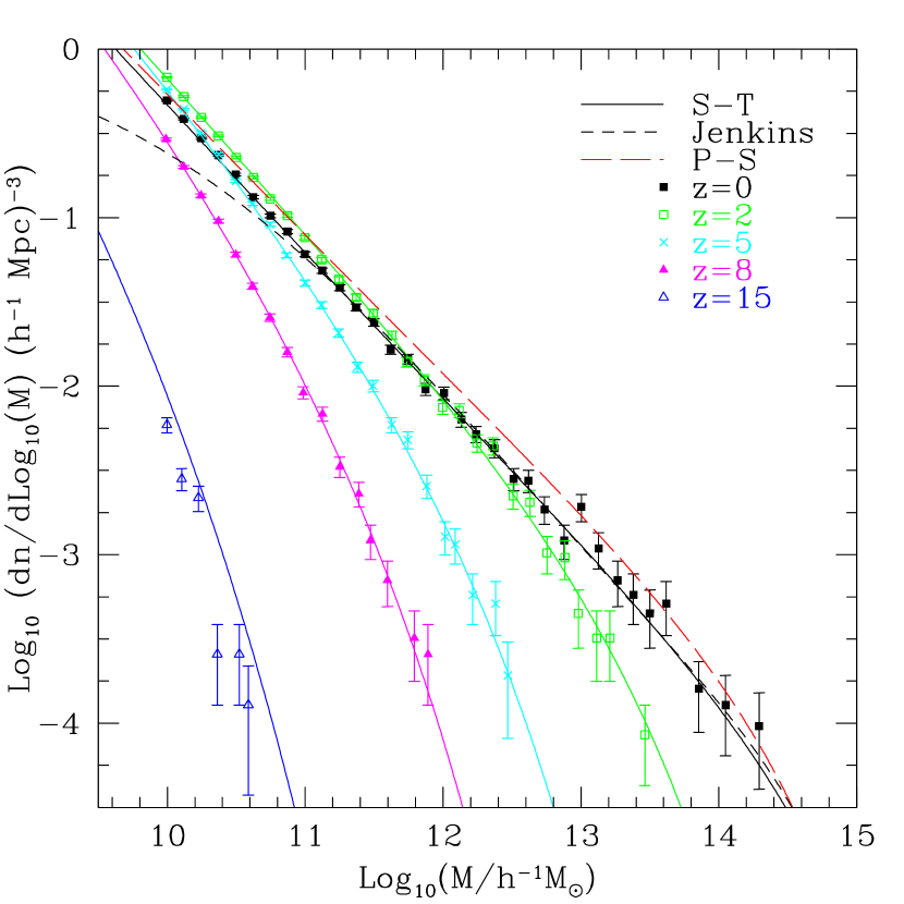
Figure 2: Comparison of the mass function per decade of mass. Data points are our $\Lambda$CDM simulation results with 1$\sigma$ poisson error bars. Throughout the paper, haloes are identified using a FOF $ll=$0.2, unless otherwise specified; only haloes with at least 64 particles are considered. In our plots, we plot the median halo mass in a bin. Solid curves are the Sheth & Tormen function at z$=$0, 2, 5, 8, & 15. Short dashed curve is the Jenkins et al. “universal” mass function (Eqn. 6), which diverges when extrapolated well below its original lower mass limit of $\simeq 4\times 10^{11}h^{-1}{\rm{M}}_{\odot}$ for our $\sigma_{8}=1.0$ model (see text). Long dashed curve is the Press & Schechter function.

In Fig. 3, we show the evolution of the mass function over all of our redshifts compared to its S-T predicted evolution. The S-T function provides an excellent fit to our data, except at very high redshifts, where it significantly overpredicts the halo abundance. At all redshifts up to z$=$10, the difference is $\lower 2.15277pt\hbox{$\;\buildrel<\over{\sim}\;$}10\%$ for each of our well sampled mass bins. However, the S-T function begins to overpredict the number of haloes increasingly with redshift for z$\;\buildrel>\over{\sim}\;$10, up to $\sim 50$% by z$=$15. The simulation mass functions appear to be generally steeper than the S-T function, especially at high redshifts. In Fig. 4, we show the evolution of the mass function over all of our redshifts as a function of $M/M_{*}$. This highlights the remarkable accuracy of the S-T mass function over more than 10 decades of $M/M_{*}$.

Figure 3: Fractional difference between our simulated mass function (FOF $ll=$0.2) and the S-T prediction. Poisson error bars shown.

Figure 4: Number density vs. M/M^∗. Data points with poisson error bars are our simulation results. Curves are S-T predictions. Redshifts plotted are (from left to right) 0, 1., 2., 3., 4., 5., 6.2, 7.8, 10., 12.1, 14.5

In Fig. 5, we plot the mass function for all of our outputs in the $f-\ln(\sigma^{-1})$ plane. Large values of $\ln\sigma^{-1}$ correspond to rare haloes of high redshift and/or high mass, while small values of $\ln\sigma^{-1}$ describe haloes of low mass and redshift combinations. In Fig. 6, we compare our simulated mass function with the S-T prediction, by plotting the residuals over our entire range. We limit plotted data to bins with poisson errors of less than 20%. Remarkably, the S-T function fits our simulated mass function to better than 10$\%$ over the range of -1.7 $\leq\ln\sigma^{-1}\leq$ 0.5. We are unaware of any previous studies that probe the mass function down to such low values of $\ln\sigma^{-1}$ in a cosmological environment. The S-T function appears to significantly overpredict haloes for $\ln\sigma^{-1}\geq$ 0.5. This is the same overprediction seen in the number density for $z\geq 10$ in figs. 3 and 4. The large apparent scatter of the mass function for ln$\sigma^{-1}\lower 2.15277pt\hbox{\mbox{$\;\buildrel>\over{\sim}\;$}}$ 0.5 is due to larger poisson errors in this range. For large ln$\sigma^{-1}$, we estimate the uncertainty in the mass function due to cosmic variance by estimating the contribution of linear fluctuations on the scale of the box size. Cosmic variance can have large effects on results since it has the potential to increase or decrease the mass function in multiple mass bins simultaneously, and cosmic variance is difficult to quantify without a large set of simulated volumes. In our estimation, we use a second order Taylor expansion of $f(\sigma;{\rm S{\rm-}T})$, ignoring the first order term since we have imposed the average density of our simulation to be $\Omega_{m}$. The resulting estimate for the uncertainty in the mass function due to cosmic variance is $\Delta_{f,c.v.}\sim{{\partial^{2}f(\sigma;{\rm S{\rm-}T})}\over\partial\sigma^{2}}{1\over{2}}{\sigma_{Mbox}^{2}}$, which we evaluate numerically. In our well sampled, low redshift mass bins, $\Delta_{f,c.v.}$ is negligible. For our highest redshift results, $\Delta_{f,c.v.}$ is smaller than our poisson error limit of 20$\%$ for figures 6 and 7, even for our highest mass bins. However, $\Delta_{f,c.v.}$ approaches our poisson error limit of 20$\%$ for our $z=$14.5 output. For our $z=$10 and $z=$12 outputs, $\Delta_{f,c.v.}$ is less than 10$\%$ in bins where poisson errors are less than 10$\%$, which is the case for most of our bins at that redshift. Thus, while cosmic variance is a significant source of error where the mass function is steepest, it is unlikely to entirely account for our discrepancy with the S-T function. We note that several of our $z<2$ points lie roughly 3$\sigma$ above the mean; this is actually just one mass bin plotted repeatedly at different redshifts, and so is not entirely surprising. By careful examination of ranges of ln$\sigma^{-1}$ where outputs of different redshifts overlap, we verify that the magnitude of the S-T overprediction at high values of ln$\sigma^{-1}$ is consistent with being a function purely of ln$\sigma^{-1}$ rather than redshift, a natural consequence of the fact that the mass function is self similar in time (e.g. Efstathiou et al. 1988; Lacey & Cole 1994; Jenkins et al. 2001). Jenkins et al. (2001) also find an overprediction by the S-T function for $\ln\sigma^{-1}\lower 2.15277pt\hbox{\mbox{$\;\buildrel>\over{\sim}\;$}}0.75$, which with their larger simulation volumes, corresponded primarily to objects of z$\leq$2 and of much higher mass. Additionally, Jenkins et al. find the mass function to be invariant with redshift within their own results. In Fig. 7, we compare a subset of our data with the Jenkins et al. “universal” mass function. We note that when extrapolated to $\ln\sigma^{-1}\leq-1.4$, well below its empirical fit range of $-1.2\leq\ln\sigma^{-1}\leq 1.05$, the Jenkins et al. function diverges from our results, reflecting the fact that it is of a form not ideally suited for extrapolation. Where our data overlap ($\ln\sigma^{-1}\geq-1.2$), we find generally good agreement, although we have $\sim 20\%$ fewer haloes and a somewhat steeper mass function at $\ln\sigma^{-1}\lower 2.15277pt\hbox{\mbox{$\;\buildrel>\over{\sim}\;$}}0.25$. Over the range of -1.4 $\lower 2.15277pt\hbox{$\;\buildrel<\over{\sim}\;$}\ln\sigma^{-1}\lower 2.15277pt\hbox{$\;\buildrel<\over{\sim}\;$}$ 0.75, the Jenkins et al. mass function matches our data to within $\simeq 20\%$.

We consider the possibility that this difference between our data and the Jenkins et al. fit could be due to differences in the effective slope of the power spectrum, n_eff, where $P(k)\propto k^{n_{eff}}$. Applying a simple power law to Eqn. 2 yields $\sigma^{2}\propto M^{-(n_{eff}+3)/3}$, which can be reparameterized as

$$n_{\rm eff}=6{{\rm d}\ln\sigma^{-1}\over{\rm d}\ln M\phantom{+}}-3,$$ (8)

(Jenkins et al. 2001). Fig. 8 shows the $n_{eff}~{}vs.~{}\ln\sigma^{-1}$ parameter space that our results cover. Our data generally has a steeper $n_{eff}$ than Jenkins et al., though there is some overlap, especially at lower redshifts. Since the slope of the linear power spectrum is invariant with redshift for a given $k$, n${}_{eff}(z)$ is constant for a given mass, meaning that for our lowest mass haloes we sample nearly all of our $f(\sigma)$ at an n${}_{eff}\simeq-2.3$. If we consider $n_{eff}(\sigma=0.5)$, where the power spectrum begins to go nonlinear, then we find that our results differ significantly from the Jenkins et al. function only where $n_{eff}$ at the nonlinear scale is steepest. In particular, the disagreement is worst at z$\geq$10 where $n_{eff}(\sigma=0.5)$ exceeds their maximum value of -2.26. Thus, there is a possibility that our steeper values of n_eff results in an $f(\sigma)$ with a slightly different shape, which might account for the difference with prior results, but a larger set of simulations with still steeper $n_{eff}$ would be needed to clearly show any such dependence.

Figure 5: Mass function plotted in redshift independent form for all of our outputs as in Fig. 4. Solid curve is S-T prediction.

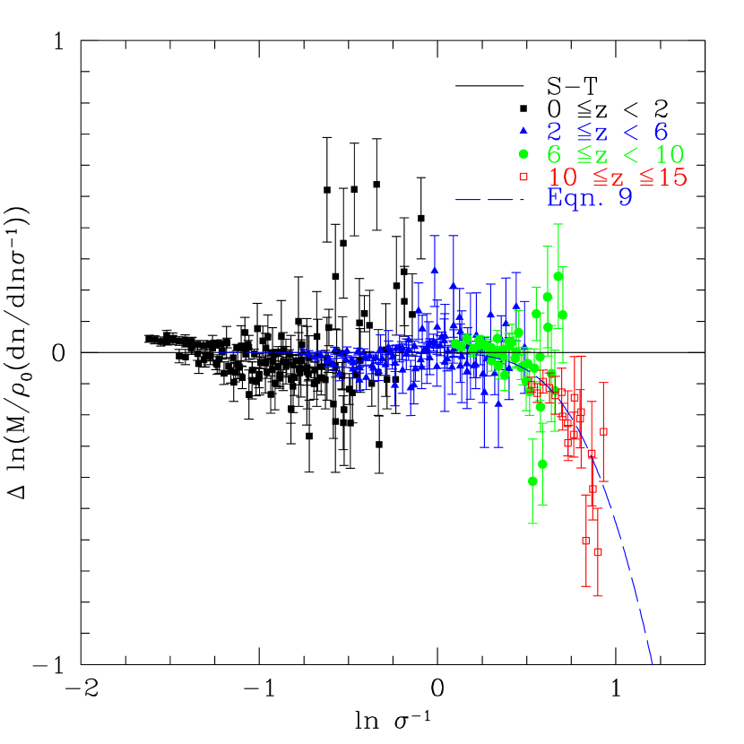
Figure 6: Residuals between S-T prediction and our results for the mass function of Fig. 5 (with FOF $ll$=0.2). Solid straight line is the S-T function. Dashed line is our empirical adjustment to the S-T function.

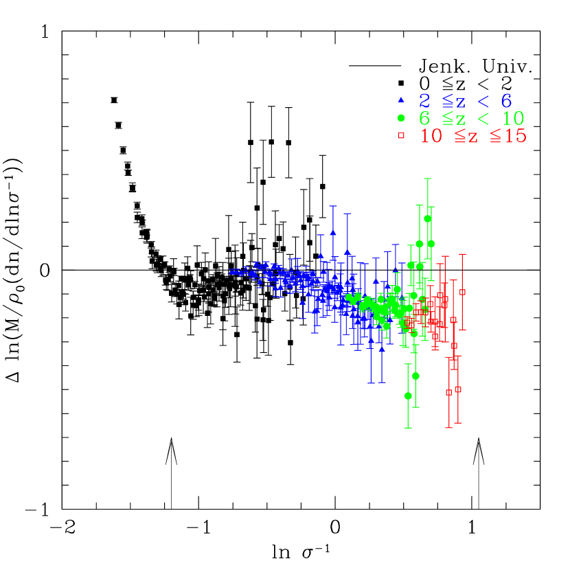
Figure 7: Residuals between Jenkins et al. mass function and our results for the mass function of Fig. 5. Arrows encompass the range of data used in the Jenkins et al. empirical fit, which is denoted by the solid straight line.

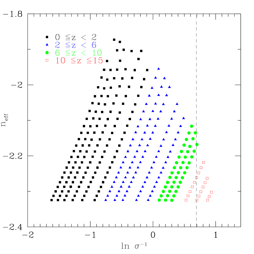
Figure 8: Parameter range covered by our results. Each mass bin for which we have poisson statistics of better than 20$\%$ error is shown. The vertical line denotes $\sigma=0.5$.

Since no mass function that we have considered is accurate for the entire range of our data, we consider the possibility of an empirical adjustment to the S-T function. We insert a crude multiplicative factor to the S-T function as follows, with $\delta_{c}$ $=$ 1.686 and FOF $ll=$0.2 (Fig. 6):

$$f(\sigma)=f(\sigma;{\rm S{\rm-}T})\bigg{[}exp[-0.7/(\sigma[\cosh(2\sigma)]^{5})]\bigg{]},$$ (9)

valid over the range of -1.7 $\leq\ln\sigma^{-1}\leq$ 0.9. The resulting function is virtually identical to the S-T function for all $-\infty\leq\ln\sigma\leq 0.4$. At higher values of $\ln\sigma^{-1}$, this function declines relative to the S-T function, reflecting an underabundance of haloes that becomes greater with increasing $\ln\sigma^{-1}$. For -1.7 $\leq\ln\sigma^{-1}\leq$ 0.5, Eqn. 9 matches our data to better than 10$\%$ for well-sampled bins, while for 0.5 $\leq\ln\sigma^{-1}\leq$ 0.9, where poisson errors are larger, our data is matched to roughly 20$\%$. We must caution that though Eqn. 9 is a good fit to our data, it differs from the S-T function in the regime where poisson and cosmic errors are highest, and where our results are most prone to potential numerical errors because of the steepness of the mass function. Our results are more robust in the low $\ln\sigma^{-1}$ regime. Note that in the Eqn. 9 fit, not all mass belongs to a halo, so Eqn. 3 is not valid.

4.1 Friends-of-Friends (FOF) versus Spherical Overdensity (SO)

Other authors have noted the advantages and disadvantages of the FOF and SO algorithms (see Jenkins et al. 2001 and references therein). The FOF method has the advantage that it can identify haloes of any shape as long as their minimum local number density is at least roughly $1/b^{3}$, and FOF is generally computationally cheaper than SO. However, FOF can sometimes spuriously link together haloes that lie close together within a filament (see e.g. Governato et al. 1997). In Fig. 9, we compare FOF mass functions of our simulation with the corresponding SO mass functions for a range of redshifts. Note that the vertical axes are somewhat arbitrary for the z$=$10 and z$=$15 outputs as these were made from the z${}_{0}=69$ version of the simulation which had a somewhat suppressed mass function, which we discuss in section 4.2. The halo finders have excellent agreement at low redshifts, with differences of $\lower 2.15277pt\hbox{$\;\buildrel<\over{\sim}\;$}10\%$ over the range where the mass function is well sampled. Differences in the high mass bins are due to a combination of different mass calculations for individual selected clusters as well as offset mass bins. The steep dropoff in the SO mass function for low masses is due to a our exclusion of SKID haloes of less than 64 particles as potential SO centers. At high redshifts, FOF $ll=$0.2 produces a substantially higher mass function than FOF $ll=$0.164 or SO, which are similar to each other, implying sensitivity to $ll$ for large $\ln\sigma^{-1}$, probably because the mass function is steep there, and thus sensitive to halo selection criteria. To verify that the discrepancy of FOF $ll=$0.2 with SO is not due simply to our choice of using skid haloes as our initial SO centers, we have included a high redshift (z$=$10) SO mass function which uses FOF haloes as initial SO centers; our choice of centers from which to grow our SO spheres has no effect on the SO mass function. A visual inspection in which halo members are “marked”, reveals that at high redshift, FOF $ll=$0.2 links together some neighboring haloes connected by filaments, but FOF also identifies some individual haloes (often of highly elongated shape) that are missed by SO, so neither algorithm is ideal. The overprediction of the S-T function for rare objects worsens somewhat if we use SO derived mass functions. Using a linking length that varies with redshift in an attempt to match the varying overdensity of virialized haloes, would have little effect on our mass function, since at low redshift the mass function is insensitive to $ll$, and at high redshift $\Omega_{m}\simeq$1, implying $ll=$0.2 (Davis et al. 1985; Lacel & Cole 1994). However, had we sampled large $\ln\sigma^{-1}$ at low redshift, adjusting $ll$ to match virial overdensity would likely have a significant effect.

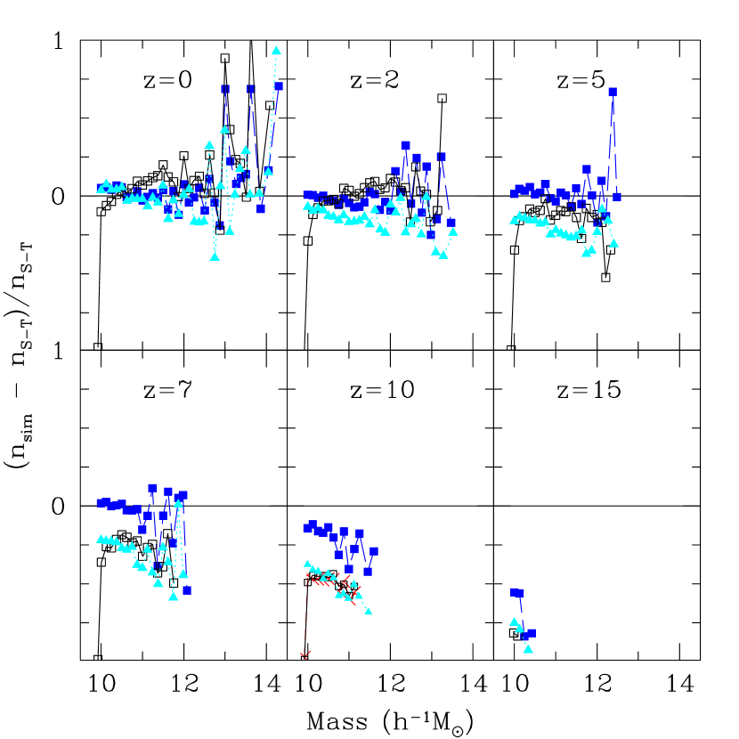
Figure 9: Comparison of SO and FOF mass functions from our simulation. Filled squares (connected by dashed lines) are for FOF $ll=$0.2 haloes; filled triangles (connected by dotted lines) are FOF $ll=$0.164 haloes. Open squares (solid lines) are SO haloes made with SKID centers. X’s at z$=$10 are SO haloes made using FOF centers. SO overdensity criterion is from Kitayama & Suto 1996. Note that the $z=10$ and $z=15$ data lie too far below the S-T function in this plot because it is from our z${}_{0}=$69 run rather than our z${}_{0}=$139 run, which we use for the rest of the high redshift results of this paper.

4.2 Numerical Tests

We check that the disagreement of S-T which appears at high redshift is not a result of delayed halo collapse due to numerical errors that can be caused by too large of a gravitational softening length. We make additional checks addressing potential numerical errors caused by mapping particles with Zel‘dovich displacements (Zel’dovich 1970) onto a particle grid; an insufficiently high starting redshift could delay collapse of the first haloes (e.g. Jenkins et al. 2001). If initial conditions are set with some regions having overdensities high enough to already be in the non-linear regime, then the linear Zel‘dovich mapping can not account for shell-crossing wherein mass piles up as it flows toward overdensities. The effects of either of these error sources, if present, should have evolved away by lower redshifts, since the tiny fraction of matter that is in haloes at such high redshifts is soon incorporated into clusters or large groups.

Table 1: N-body simulation parameters, including test runs

z0	$r_{\rm soft}(h^{-1}{\rm kpc}$)	$\Theta$(z$>$7)	nreplica	zevolved:	$\Theta$(2$<$z$<$7)	$\Theta$(z$<$2)
69	5.0	0.7	1	0	0.7	0.8	Applied to z$<$7 results; SO vs. FOF test
139	5.0	0.5	1	7	–	–	Applied to z$\geq$7 results
139	5.0	0.5	2	7	–	–	Test
69	2.5	0.7	1	7	–	–	Test
39	5.0	0.7	1	10	–	–	Test
279	5.0	0.5	2	7	–	–	Test

Table 1 lists our test runs, each of which consists of an identical 432³ particle volume with identical random waves, and is evolved to z$=$7. Fig. 10 shows the mass function for z$\simeq$7-15 for our low softening test run, started from z${}_{0}=$69, and plotted relative to the S-T function along with our z${}_{0}=$69, 5 $h^{-1}$kpc data. Halving the softening to 2.5 $h^{-1}$kpc has no effect on the mass function. Fig. 11 shows the mass function for z$\simeq$7-15 for our initial redshift test runs, all with 5 $h^{-1}$kpc softening. Lowering the initial redshift to 39 substantially reduces the number of high redshift haloes, so we did not evolve the z${}_{0}=$39 run to z$<$10. The z${}_{0}=$139 run matches the z${}_{0}=$279 run, indicating convergence, but the z${}_{0}=$69 run has a reduced mass function relative to the z${}_{0}=$139 run at redshifts z$\;\buildrel>\over{\sim}\;$12. By z$=$7, however, the z${}_{0}=$139 and z${}_{0}=$69 mass functions have converged, showing that evolving the simulation over an expansion factor of $\simeq$10 from initial conditions is sufficient for mass function measurements. We consequently derive our low redshift (z$<$7) results throughout this paper from the z${}_{0}=$69, 5 $h^{-1}$kpc simulation, and utilize the z${}_{0}=$139 run for our z$\geq$7 results. We make an additional test of z$\geq$7 cell opening angle, which is used to determine how accurately long range gravitational forces are to be approximated. If the cell opening angle is too large, then artificial net forces will be incurred upon particles, which could cause “spurious” haloes to form. This effect is most likely to occur at high redshifts when gravitational perturbations are small and force errors are fractionally larger. Decreasing the opening angle from $\Theta$=0.7 to $\Theta$=0.5, for our z${}_{0}=$139 case, had no appreciable effect on the mass function for z$\geq$7. We test that the number of replicas used for our periodic boundaries, n${}_{r}=$1, is adequate. With z${}_{0}=$139, increasing n_r from 1 to 2 has no effect on the mass function. Additionally, to test that our box size is adequate, we have verified that our z$=$0 mass function agrees with the mass function from larger, lower resolution volumes where they overlap (not included in Table 1).

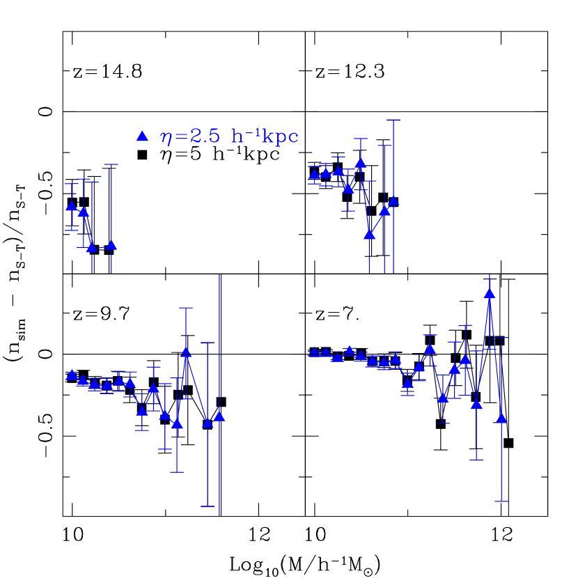
Figure 10: The high redshift mass functions for runs with softening lengths of 5 $h^{-1}$kpc and 2.5 $h^{-1}$kpc. Both runs were started from a redshift of 69.

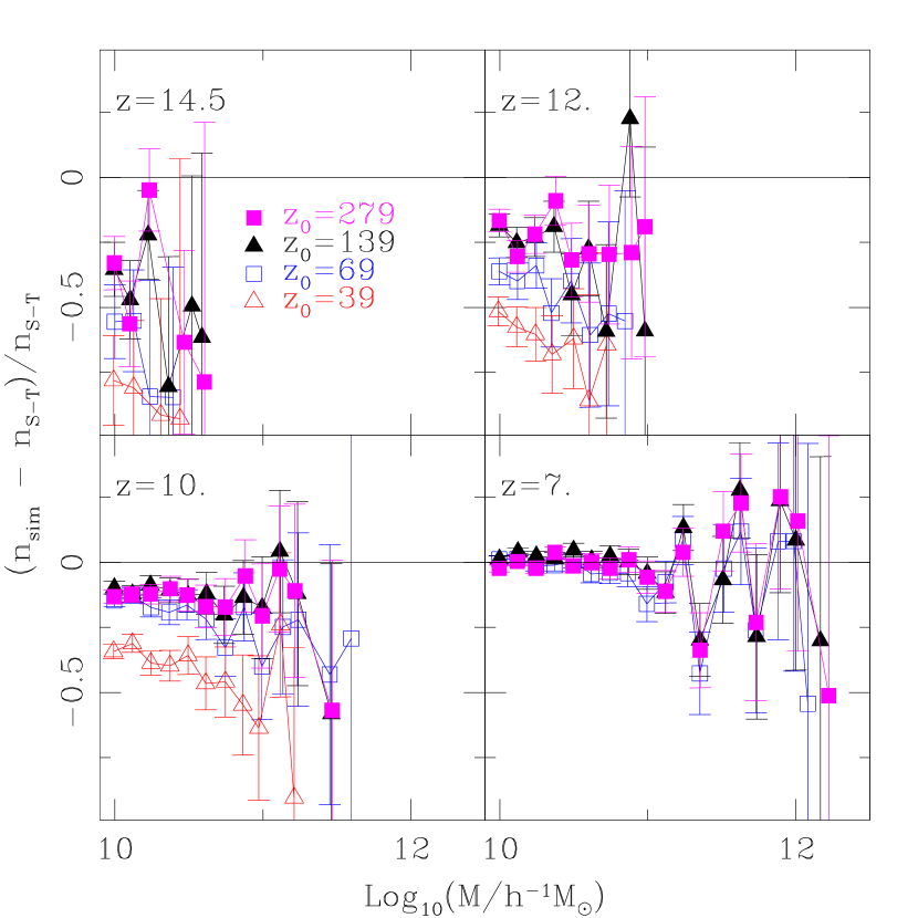
Figure 11: The high redshift mass functions for initial redshifts of 39, 69, 139, and 279. Each run has a softening of 5 $h^{-1}$kpc. The $z_{0}=$39 run was stopped at $z=$10.

5 Conclusions

Our results extend to lower masses and higher redshifts than the original empirical fit of the S-T mass function. The range of masses and redshifts over which the S-T mass function remains valid is quite remarkable, and though it does begin to break down at redshift $\;\buildrel>\over{\sim}\;$ 10 in our results, no other function matches its range and accuracy. It is not well understood why the mass function can be described so well by solely $\sigma(M)$. Lacey & Cole 1994, in simulations with scale free power spectra, found evidence that the mass function depends on n_eff as well as $\sigma$, though they tested a wider range in n_eff than in more recent CDM simulations. The generally good agreement of our data with previous work at much shallower n_eff implies that any such dependence is weak, though it may be manifested in our results where we differ from the S-T function. As n_eff approaches -3, the growth of M_∗ with time diverges, so any dependence of f($\sigma$) on n_eff is most likely to occur near that regime. Simulations with finer mass resolution will be able to test yet steeper values of n_eff. Based on the apparent trend of the S-T function to overpredict halo numbers for objects of greater rarity, we expect that the overprediction of the S-T function may continue to worsen when even higher values of $\ln\sigma^{-1}$, or equivalently, when more extreme values of $M/M_{*}$ and redshift, are analyzed. Theoretical work that focuses on halo collapse in this high $\ln\sigma^{-1}$ range is needed to produce more robust predictions.

Because the form of the mass function for low mass, low redshift haloes closely resembles a power law, we are cautiously optimistic that the S-T mass function will continue to provide a good match to simulation data as lower values of $\ln\sigma^{-1}$ are modeled, though this extrapolation will likely breakdown where n_eff approaches -3. Simulations that model higher particle numbers (leading to higher redshifts), are needed to extend the known range of the mass function of dark matter haloes. The accuracy of the S-T function for low mass haloes out to high redshifts has important implications for a number of astrophysical problems. Evolution of the mass and luminosity functions down to dwarf scales permits comparison with surveys, providing important cosmological tests, and allows calculations of merger histories and star formation histories of galaxies, groups, and clusters. Our results verify that the S-T function is accurate over the entire evolutionary range (for which progenitors or descendants are observable) of lyman break galaxies and groups of galaxies. Assuming a weak dependence on n_eff, the redshift invariance of the mass function implies that extrapolation of mass functions should be reliable for combinations of masses and redshifts that cannot presently be simulated, as long as only values of $\ln\sigma^{-1}$ that have been verified by simulation are considered. The number densities of low mass ($<10^{10}{\rm{M}}_{\odot}$) haloes at high redshift (z $\sim$ 10), needed for studies of reionization, or galaxy formation (e.g. Haiman 2002), should be well described by the S-T function since although they lie below our mass range, they are within our range of simulated $\ln\sigma^{-1}$. For such extrapolation to be accurate down to indefinitely small masses, all mass would have to be in dark matter haloes of some mass or else low mass haloes would be overpredicted.

Extrapolation of mass functions to large values of $\ln\sigma^{-1}$ that have yet to be verified by simulations, however, are likely to be significantly in error, as suggested by the trend of increasing overprediction by the S-T function for high values of $\ln\sigma^{-1}$. Though our results only reach $\simeq$4$\sigma$ density peaks, there is a trend for the S-T function to increasingly overpredict the mass function for increasing $\sigma$ beginning at $\simeq$3$\sigma$. The discrepancy with the S-T function for rare objects has significant implications for studies that make use of such rare objects as a cosmological probe. For example, the number density of high redshift (z $\simeq$ 6) QSOs, which are thought to be hosted by haloes at 5$\sigma$ peaks in the fluctuation field (Haiman & Loeb 2001; Fan et al. 2001), are likely to be overpredicted by at least a factor of 50$\%$. Some uncertainty is also introduced for studies employing the abundance of the highest redshift clusters to probe cosmological parameters (e.g. Robinson, Gawiser, & Silk 2000 and references therein).

5.1 Summary

In summary, we have utilized high resolution simulations to derive the mass function of dark matter haloes over an extended range in both mass and redshift over previous work. We find that the S-T mass function holds up exceptionally over more than 10 orders of magnitude of $M/M_{*}$. For -1.7 $\leq\ln\sigma^{-1}\leq$ 0.5, the S-T mass function is an excellent fit to our data, but begins to overpredict haloes for ln$(\sigma^{-1})\lower 2.15277pt\hbox{\mbox{$\;\buildrel>\over{\sim}\;$}}$ 0.5, or $M/M_{*}$ $\;\buildrel>\over{\sim}\;$ 10⁶ in our volume, reaching a $\sim$50$\%$ discrepancy by ln$(\sigma^{-1})\simeq$ 0.9, corresponding to $M/M_{*}$ $\sim$ 10⁹ at z$\simeq$15 in our volume. We offer an empirical adjustment for the high ln$(\sigma^{-1})$ portion of the S-T mass function. Our results confirm the redshift invariance of the mass function.

References

- (1) Bardeen, J.M., Bond, J.R., Kaiser, N., Szalay, A.S., 1986, ApJ, 305, 15.
- (2) Bond J.R., Cole S., Efstathiou G., Kaiser N., 1991, ApJ, 379, 440
- (3) Bower, R.G., 1991, MNRAS, 248, 332
- (4) Davis, M., Efstathiou, G., Frenk, C.S., White, S.D.M., 1985, ApJ, 292, 381
- (5) Efstathiou, G., Frenk, C.S., White, S.D.M., Davis, M., 1988, MNRAS, 235, 715
- Eke et al. (1996) Eke, V.R., Cole, S., Frenk, C.S., 1996, MNRAS, 282, 263
- Evrard et al. (2002) Evrard, A., et al. , 2002, ApJ, 573, 7
- Fan et al. (2001) Fan, X. et al. , 2001, AJ, 122, 2833
- Gardner (2001) Gardner, J.P., 2001, ApJ, 557, 616
- (10) Governato, F., Moore, B., Cen, R., Stadel, J., Lake, G., Quinn, T., 1997, NewA, 2, 91
- (11) Governato, F., Baugh, C., Frenk, C., Cole, S., Lacey, C., Quinn, T., Stadel, J., 1998, Nature, 392, 359.
- Governato et al. (1999) Governato F., Babul A., Quinn T., Tozzi P., Baugh C. M., Katz N., Lake G., 1999, MNRAS, 307, 949
- Governato et al. (2001) Governato F., Ghigna, S., Moore, B., Quinn T., Stadel, J., Lake G., 2001, ApJ, 547, 555
- (14) Gross, M.A., Somerville, R.S., Primack, J.R., Holtzman, J., Klypin, A., 1998, MNRAS, 301, 81
- (15) Haiman, Z., 2002, ESO Astrophysic Symposium, astro-ph 0201173
- (16) Haiman, Z., Loeb, A., 2001, ApJ 552, 459
- (17) Jenkins A., Frenk C.S., Pearce F.R., Thomas, P.A., White, S.D.M., Couchman H.M.P., Peacock, J.A., Efstathiou, G., Neson, A.H., 1998, ApJ, 499, 20
- (18) Jenkins A., Frenk C.S., White S.D.M., Colberg J.M., Cole S., Evrard A.E., Couchman H.M.P., Yoshida N., 2001, MNRAS, 321, 372
- (19) Kitayama, T., Suto, Y., 1996, MNRAS, 469, 480.
- (20) Lacey C., Cole S., 1993, MNRAS, 262, 627
- (21) Lacey C., Cole S., 1994, MNRAS, 271, 676
- (22) Lee J., Shandarin S.F., 1998, ApJ, 500, 14
- (23) Monaco P., 1997a, MNRAS, 287, 753
- (24) Monaco P., 1997b, MNRAS, 290, 439
- (25) Monaco P., Theuns, T., Taffoni, G., Governato, F., Quinn, T., & Stadel, J., 2002, ApJ, 564, 8.
- (26) More, J., Heavens A., Peacock, J., 1986, MNRAS 220, 189
- (27) Nagashima, M., 2001, ApJ, 562, 7.
- (28) Peebles P.J.E., 1993, Principles of Physical Cosmology, Princeton University Press, Princeton
- (29) Press W.H., Schechter P., 1974, ApJ, 187, 425
- (30) Ratra, B., Sugiyama, N., Banday, A.J., Gorski, K.M., 1997, ApJ, 481, 22
- (31) Robinson, J., Gawiser, E., Silk, J., 2000, ApJ, 532, 1 1997, ApJ, 481, 22
- (32) Sheth R.K., Mo H., Tormen G., 2001, MNRAS, 323, 1
- Sheth & Tormen (1999) Sheth R. K., Tormen G., 1999, MNRAS, 308, 119
- (34) Stadel, J, 2001, PhDT.
- (35) Steidel, C. C., Giavalisco, M., Pettini, M., Dickinson, M., Adelberger, K., 1996, ApJ, 162, L17.
- (36) White M., 2002, ApJS, 143, 241.
- (37) Williams, R., et al. 1996, AJ, 112, 1335
- (38) Yano, T., Nagashima, M., & Gouda, N., 1996, ApJ, 466, 1.
- (39) Zel’dovich YA. B., 1970, Astrofizika, 6, 319 (translated in Astrophysics, 6, 164 [1973])