Near-Infrared Interferometric Measurements of Herbig Ae/Be Stars

Abstract

We have observed the Herbig Ae/Be sources AB Aur, VV Ser, V1685 Cyg (BD+40^∘4124), AS 442, and MWC 1080 with the Palomar Testbed Interferometer, obtaining the longest baseline near-IR interferometric observations of this class of objects. All of the sources are resolved at 2.2 $\mu$m with angular size scales generally $\lesssim 5$ mas, consistent with the only previous near-IR interferometric measurements of Herbig Ae/Be stars by Millan-Gabet and collaborators. We determine the angular size scales and orientations predicted by uniform disk, Gaussian, ring, and accretion disk models. Although it is difficult to distinguish different radial distributions, we are able to place firm constraints on the inclinations of these models, and our measurements are the first that show evidence for significantly inclined morphologies. In addition, the derived angular sizes for the early type Herbig Be stars in our sample, V1685 Cyg and MWC 1080, agree reasonably well with those predicted by the face-on accretion disk models used by Hillenbrand and collaborators to explain observed spectral energy distributions. In contrast, our data for the later-type sources AB Aur, VV Ser, and AS 442 are somewhat inconsistent with these models, and may be explained better through the puffed-up inner disk models of Dullemond and collaborators.

1 Introduction

Herbig Ae/Be (HAEBE; Herbig, 1960) stars are intermediate-mass (2–10 M_⊙) young stellar objects that show broad emission lines, rapid variability, and excess infrared and millimeter-wavelength emission. These properties are consistent with the presence of hot and cold circumstellar dust and gas. While there is still some debate about the morphology of this circumstellar material, most evidence supports the hypothesis that in many cases the dust and gas lies in a massive ($\sim 0.01$ M_⊙) circumstellar disk (Natta, Grinin, & Mannings 2000; Hillenbrand et al. 1992, hereafter HSVK).

The strongest evidence for circumstellar disks around HAEBE stars comes from direct imaging with millimeter interferometry. Flattened structures around several sources have been resolved on $\sim 100$ AU scales (Mannings & Sargent, 1997, 2000; Piétu et al., 2003), and detailed kinematic modeling of one source, MWC 480, shows that the observations are fit well by a rotating Keplerian disk (Mannings et al., 1997). For a spherical distribution, these and other observations (e.g., Mannings, 1994) imply extinctions at visible and infra-red wavelengths much higher than actually observed. In addition, in recent H$\alpha$ spectropolarimetric observations of HAEBE sources (which trace dust on scales of tens of stellar radii), Vink et al. (2003) find signatures of flattened circumstellar structures around 83% of their sample, and evidence for rotation around 9 HAe stars. Furthermore, the forbidden emission lines that arise in winds and outflows around HAEBE sources typically show blue-shifted emission but lack redshifted emission, which suggests that the redshifted component of the outflow is occluded by a circumstellar disk. The broad linewidths of low-velocity features are consistent with this emission arising in rotating circumstellar disk winds (Corcoran & Ray, 1997).

The distribution of circumstellar material around HAEBEs can also be inferred from modeling of spectral energy distributions (SEDs). Three distinct morphologies were identified in this way by HSVK, who classified observed HAEBE sources into three groups, I, II, and III. All sources in our observed sample fall into Group I, which has SEDs of the form $\lambda F_{\lambda}\propto\lambda^{4/3}$. These can be modeled well by flat, irradiated, accretion disks with inner holes on the order of $\sim 10$ stellar radii. Recent SED modeling of a sample of fourteen isolated HAEBE stars with the characteristics of Group I sources is consistent with emission from a passive reprocessing disk (Meeus et al., 2001). Moreover, Meeus et al. (2001) (and other investigators, e.g., Natta et al., 2001) attribute this emission to the outer part of a flared circumstellar disk (e.g., Chiang & Goldreich, 1997), while previous authors attributed blackbody components observed in SEDs of HAEBE sources to tenuous envelopes (Hartmann et al., 1993; Miroshnichenko et al., 1999; Natta et al., 1993).

Size scales and orientations of disks around HAEBE stars can only be determined directly through high angular resolution imaging. The spatial and velocity structure of cooler outer HAEBE disks on $\sim 100$ AU scales has been mapped with millimeter-wave interferometers (as discussed above). To probe the warmer inner regions of the disk ($\sim 1$ AU scales), measurements with near-IR interferometers are necessary. The only near-IR interferometric observations of HAEBE sources to date, conducted with the IOTA interferometer (Millan-Gabet et al. 1999; Millan-Gabet, Schloerb, & Traub 2001, hereafter MST), led to sizes and orientations of sources largely inconsistent with values estimated using other techniques. A geometrically flat disk may be too simplistic to accommodate all the observations, and puffed up inner disk walls (Dullemond, Dominik, & Natta 2001; hereafter DDN) or flared outer disks (e.g., Chiang & Goldreich, 1997) may need to be included in the models. However, the limited number of HAEBE sources observed with near-IR interferometers and the sparse $u-v$ coverage of these observations (MST, ) make it difficult to draw unambiguous conclusions about the structure of the circumstellar material.

We have begun a program with the Palomar Testbed Interferometer (PTI) to observe HAEBE stars. By increasing the sample size and improving $u-v$ coverage, we aim to understand better the structure of the circumstellar emission on $\sim 1$ AU scales. In this paper, we present results for five sources, AB Aur, VV Ser, V1685 Cyg (BD+40^∘4124), AS 442, and MWC 1080. We note that neither our list of HAEBEs, nor that of MST, represents an unbiased sample, but rather, is limited to those stars that are bright enough ($K\lesssim 6.5$) to be successfully observed. We model the structure of circumstellar dust around HAEBE stars using these PTI data, together with IOTA measurements where available. Specifically, we compare various models—Gaussians, uniform disks, uniform rings, and accretion disks with inner holes—to the visibility data to determine approximate size scales and orientations of the circumstellar emission.

In §2, we describe the PTI observations. In §3, we fit the observed data to several different models for the circumstellar dust distribution and derive angular sizes and orientations. Implications of the modeling and comparisons with previous observations are discussed in §4.

2 Observations and Calibration

The Palomar Testbed Interferometer (PTI) is a long-baseline near-IR Michelson interferometer located on Palomar Mountain near San Diego, CA (Colavita et al., 1999). PTI combines starlight from two 40-cm aperture telescopes using a Michelson beam combiner, and records the resulting fringe visibilities. These fringe visibilities are related to the source brightness distribution via the van Cittert-Zernike theorem, which states that the visibility distribution in $u-v$ space and the brightness distribution on the sky are Fourier transform pairs (Born & Wolf, 1999).

We observed five HAEBE sources, AB Aur, VV Ser, V1685 Cyg (BD+40^∘4124), AS 442, and MWC 1080, with PTI between May and October of 2002. Properties of the sample are included in Table A. We obtained K-band (2.2 $\mu$m) measurements on an 85-m North-West (NW) baseline for all five objects, and on a 110-m North-South (NS) baseline for three. The NW baseline is oriented $109^{\circ}$ west of north and has a fringe spacing of $\sim 5$ mas, and the NS baseline is $160^{\circ}$ west of north and has a fringe spacing of $\sim 4$ mas. A summary of the observations is given in Table A.

PTI measures fringes in two channels, corresponding to the two outputs from the beam combiner. One output is spatially filtered with an optical fiber and dispersed onto five “spectral” pixels, while the other output is focused onto a single “white-light” pixel (without spatial filtering). The white-light pixel is used principally for fringe-tracking: the fringe phase is measured and then used to control the delay line system to track atmospheric fringe motion (and thus maintain zero optical path difference between the two interfering beams). The spectral pixels are generally used to make accurate measurements of the squared visibility amplitudes ($V^{2}$) of observed sources. We sample the data at either 20 or 50 milliseconds in order to make measurements on a timescale shorter than the atmospheric coherence time. A “scan”, which is the unit of data we will use in the analysis below, consists of 130 seconds of data, divided into five equal time blocks. The $V^{2}$ is calculated for each of these blocks using an incoherent average of the constituent 20 or 50-ms measurements from a synthetic wide-band channel formed from the five spectral pixels (Colavita, 1999). $V^{2}$ for the entire scan is given by the mean of these five estimates, and the statistical uncertainty is given by the standard deviation from the mean value.

We calibrate the measured $V^{2}$ for the observed HAEBE sources by comparing them to visibilities measured for calibrator sources of known angular sizes, for which we can easily calculate the expected $V^{2}$ for an ideal system. The visibilities are normalized such that $V^{2}=1$ for a point source observed with an ideal system. We calculate the expected $V^{2}$ by assuming that the calibrators are uniform stellar disks. Making use of the van Cittert-Zernike theorem, the squared visibilities for these sources are given by

$$V^{2}_{\rm calc}=\left(2\frac{J_{1}(\pi\theta r_{\rm uv})}{\pi\theta r_{\rm uv}}\right)^{2}.$$ (1)

Here, $J_{1}$ is the first-order Bessel function. $\theta$ is the angular diameter of the star, and $r_{\rm uv}$ is the “uv radius”, defined by

$$r_{\rm uv}=\sqrt{u^{2}+v^{2}}=\frac{\vec{B}\cdot\vec{s}}{\lambda},$$ (2)

where $\vec{B}$ is the baseline vector, $\vec{s}$ is a unit vector pointing from the center of the baseline towards the source, and $\lambda$ is the observing wavelength. (The qualitative explanation of Equation 1 is that while for unresolved sources the visibility is constant with increasing uv radius, for progressively larger sources the visibility decreases faster with increasing uv radius.) By comparing $V^{2}_{\rm calc}$ to the measured $V^{2}$ for a calibrator, we derive the “system visibility”, which represents the point source response of the interferometer:

$$V^{2}_{\rm sys}=\frac{V^{2}_{\rm meas,calibrator}}{V^{2}_{\rm calc}}.$$ (3)

This system visibility, in turn, is used to calibrate the squared visibilities for the target source:

$$V^{2}_{\rm target}=\frac{V^{2}_{\rm meas,target}}{V^{2}_{\rm sys}}.$$ (4)

Specifically, we determine $V_{\rm sys}^{2}$ at the time of each target scan, using an average of $V_{\rm meas,calibrator}^{2}$ weighted by the proximity of the target and calibrator in both time and angle. For further discussion of the calibration procedure, see Boden et al. (1998).

Calibrators must be close to the target sources (on the sky an in time) so that the atmospheric effects will be the same for both. They should also be of small angular size, $\theta$, so that $V^{2}\rightarrow 1$ and $dV^{2}_{\rm sys}/d\theta\rightarrow 0$, and the calibration is thus less sensitive to uncertainties in the assumed calibrator diameter. The angular size of a calibrator can be estimated from the published stellar luminosity and distance, from a blackbody fit to published photometric data with the temperature constrained to that expected for the published spectral type, or from an unconstrained blackbody fit to the photometric data. We adopt the average of these three size estimates in our analysis, and the uncertainty is given by the spread of these values. Relevant properties of the calibrators used in these observations are given in Table A.

3 Results

We measured calibrated squared visibilities for AB Aur, VV Ser, V1685 Cyg, AS 442, and MWC 1080 (Table A). All five sources are resolved by PTI (i.e., $V^{2}$ is significantly different from unity), implying angular sizes $\gtrsim 1$ mas. The data are consistent with disk-like morphologies for all sources, and we can place good constraints on disk inclinations for most sources. MWC 1080, V1685 Cyg, and VV Ser show evidence for significantly non-zero inclinations, while a circularly symmetric distribution appears appropriate for AB Aur. The AS 442 data are insufficient to constrain the inclination.

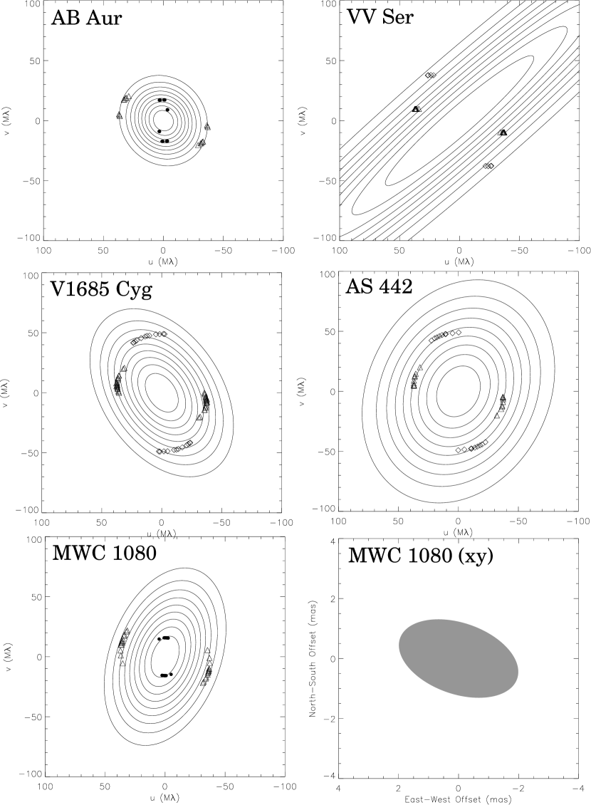
Figure 11: Contour plots of best-fit inclined uniform disk models for AB Aur, VV Ser, V1685 Cyg, AS 442, and MWC 1080, whose parameters are listed in Tables A-A. The contour increment is 10% in $V^{2}$. We also plot the best-fit inclined disk model for MWC 1080 on the sky (bottom right panel, greyscale). We over-plot the uv points sampled for each source by the PTI NW baseline (open triangles), the PTI NS baseline (open diamonds), and by IOTA (filled dots). Since we know that the brightness distributions of the sources are real, the visibilities must be reflection symmetric (through the origin), and so we also plot these reflections of the sampled uv points.

Interferometric observations of AB Aur and MWC 1080 at 2.2 $\mu$m have also been obtained with the 21-m and 38-m baselines of the IOTA interferometer (Millan-Gabet et al., 1999; MST, ). When combined with our longer baseline PTI data (85-m and 110-m), these help fill in the $u-v$ plane, and enable us to improve constraints on source models (see below; Figure 11). Based on discussion with R. Millan-Gabet, we assign an uncertainty to each IOTA visibility given by the standard deviation of all data obtained for a given source with a given baseline. We verify the registration of the IOTA and PTI data using calibrators observed by both interferometers. Since the IOTA data for AB Aur was calibrated using HD 32406, which is unresolved by both PTI and IOTA, we can be confident of the registration. We measured the diameter of HD 220074, the calibrator for MWC 1080, to be $\theta_{\rm UD}=1.98\pm 0.06$, while MST assumed a size of $2.10\pm 0.22$. This difference in angular size translates into only a 0.7% effect, which is within the measurement errors (the effect is so small because the calibrator is essentially unresolved by IOTA).

3.1 Visibility Corrections

Nearby companions that lie outside the interferometric field of view, $\sim 50$ mas, but within the field of view of the detector, $\sim 1^{\prime\prime}$, will contribute incoherent light to the visibilities. For MWC 1080, which has a known nearby companion (Corporon, 1998), we use the correction factor

$$\frac{V^{2}_{\rm true}}{V^{2}_{\rm meas}}=\left(\frac{1}{1+10^{\Delta K/2.5}}\right)^{2},$$ (5)

where $\Delta K$ is the difference in K-band magnitudes between the two stars. For MWC 1080, we measured $\Delta K=2.70$ (angular separation $=0\hbox to0.0pt{.\hss}^{\prime\prime}78$) using the Palomar Adaptive Optics system on the 200-inch telescope on November 18, 2002. V1685 Cyg is also known to have a faint companion ($\Delta K=5.50$; Corporon, 1998), but the effect of this companion on the visibilities is negligible. Adaptive optics images of the other sources in our sample show that none of these has any bright companions ($\Delta K<5$) at distances between $\sim 50$ mas and $1^{\prime\prime}$.

Our measured visibilities contain information about emission from both the circumstellar material and the star itself. We can remove the effect of the central star on the visibilities by including it in the models:

$$V^{2}_{\rm tot}=\left(\frac{F_{\ast}V_{\ast}+F_{\rm x}V_{\rm x}}{F_{\ast}+F_{\rm x}}\right)^{2}\approx\left(\frac{F_{\ast}+F_{\rm x}V_{\rm x}}{F_{\ast}+F_{\rm x}}\right)^{2},$$ (6)

where $F_{\ast}$ is the stellar flux, $F_{\rm x}$ is the excess flux (both measured at 2.2 $\mu$m), $V_{\ast}\approx 1$ is the visibility of the (unresolved) central star, and $V_{\rm x}$ is the visibility due to the circumstellar component. It is reasonable to assume that $V_{\ast}\approx 1$, since for typical stellar radii ($\sim 5$ R_⊙) and distances ($\sim 500$ pc), the angular diameters of the central stars will be $\sim 0.5$ mas. In the case of the binary model described below (§3.3.5), we do not perform any such correction, since the basic model already includes the stellar component.

Equation 6 assumes that the central star is a point source, and thus contributes coherently to the visibilities. It is also possible that the starlight is actually observable only as scattered light emission, and that it will have some incoherent contribution to the visibility ($V_{\ast}\neq 1$). For example, coronographic imaging with the Hubble Space Telescope has revealed scattered light on angular scales from $\sim 0\hbox to0.0pt{.\hss}^{\prime\prime}1$–$9^{\prime\prime}$ around AB Aur (Grady et al., 1999). A proper treatment of the effects of this scattered light on the visibilities is beyond the scope of this work, but we mention it as a possible source of uncertainty. Since the near-IR excess from HAEBE sources typically dominates over the near-IR stellar emission (§3.2; Table A), the effect should be insignificant.

3.2 Photometry

$F_{\ast}$ and $F_{\rm x}$ affect the visibilities (Equation 6), and thus it is important to determine these quantities accurately. Since HAEBE objects are often highly variable at near-IR wavelengths (e.g., Skrutskie et al., 1996), we obtained photometric K-band measurements of the sources in our sample that are nearly contemporaneous with our PTI observations, using the Palomar 200-inch telescope between November 14 and 18, 2002. Calibration relied on observations of 2MASS sources close in angle to the target sources, and we estimate uncertainties of $\sim 0.1$ magnitudes. Our photometry is consistent with published measurements to within $\sim 0.3$ magnitudes for all objects (HSVK, ; Eiroa et al., 2001).

Following HSVK and MST, we calculate $F_{\ast}$ and $F_{\rm x}$ using our K-band photometry (Table A) combined with BVRI photometry, visual extinctions, and stellar effective temperatures from the literature (HSVK, ; Oudmaijer et al., 2001; Eiroa et al., 2001; Bigay & Garnier, 1970). De-reddening uses the extinction law of Steenman & Thé (1991). Assuming that all of the short-wavelength flux is due to the central star, we fit a blackbody at the assumed effective temperature to the de-reddened BVRI data. The K-band stellar flux is derived from the value of this blackbody curve at 2.2 $\mu$m. The excess flux is then given by the difference between the de-reddened observed flux and the stellar flux. The derived fluxes are given in Table A. We note that VV Ser and AS 442 are optically variable by $\Delta V\gtrsim 1$ magnitudes on timescales of days to months (while the other sources in our sample show little or no optical variability; Herbst & Shevchenko, 1999), and thus $F_{\ast}$ is somewhat uncertain. However, since $F_{\rm x}/F_{\ast}\gg 1$ for these objects, this uncertainty is negligible when modeling the visibilities.

3.3 Models

For each source, we compare the observed visibilities to those derived from a uniform disk model, a Gaussian model, a ring model, and an accretion disk model with an inner disk hole (all models are 2-D). If we assume that the inclination of the circumstellar material is zero, then the one remaining free parameter in the models is the angular size scale, $\theta$. When we include inclination effects, we fit for three parameters: size ($\theta$), inclination angle ($\phi$), and position angle ($\psi$). Inclination is defined such that a face-on disk has $\phi=0$, and $\psi$ is measured east of north. Following MST, we include $\phi$ and $\psi$ in our models of the brightness distribution via a simple coordinate transformation:

$$x^{\prime}=x\sin\psi+y\cos\psi;\>y^{\prime}=\frac{y\cos\psi-x\sin\psi}{\cos\phi}.$$ (7)

Here, $(x,y)$ are the coordinates on the sky, and $(x^{\prime},y^{\prime})$ are the transformed coordinates. The effect of this coordinate transformation on the visibilities will be to transform $(u,v)$ to $(u^{\prime},v^{\prime})$:

$$u^{\prime}=u\sin\psi+v\cos\psi;\>v^{\prime}=\cos\phi(v\sin\psi-u\cos\psi).$$ (8)

Substitution of $(x^{\prime},y^{\prime})$ for $(x,y)$, and $(u^{\prime},v^{\prime})$ for $(u,v)$ in the expressions below yield models with inclination effects included.

In addition to these four models, we also examine whether the data are consistent with a wide binary model, which we approximate with two stationary point sources. For this model, the free parameters are the angular separation ($\theta$), the position angle ($\psi$), and the brightness ratio of the two components ($R$).

3.3.1 Gaussian Model

The brightness distribution for a normalized Gaussian model is given by

$$I_{\rm gauss}(x,y)=\exp\left(-\frac{4\ln 2\>\>(x^{2}+y^{2})}{\theta^{2}}\right),$$ (9)

and the (normalized) visibilities expected for this observed brightness distribution are calculated via a Fourier transform to be,

$$V_{\rm gauss}(r_{\rm uv})=\exp\left(-\frac{\pi^{2}\theta^{2}r_{\rm uv}^{2}}{4\ln 2}\right).$$ (10)

Here, $(x,y)$ are the angular offsets from the central star, $\theta$ is the angular FWHM of the brightness distribution, and $r_{\rm uv}=(u^{2}+v^{2})^{1/2}$ is the “uv radius” (Equation 2). The model for the observed squared visibilities is obtained by using Equation 6 with $V_{\rm x}=V_{\rm gauss}$.

3.3.2 Uniform Disk Model

The brightness distribution for a uniform disk is simply given by a 2-D top-hat function. Thus, the normalized visibilities are given by

$$V_{\rm uniform}(r_{\rm uv})=2\frac{J_{1}(\pi\theta r_{\rm uv})}{\pi\theta r_{\rm uv}},$$ (11)

where $\theta$ is the angular diameter of the uniform disk brightness distribution, and $r_{\rm uv}=(u^{2}+v^{2})^{1/2}$ is the “uv radius” (Equation 2). The model for the observed squared visibilities is obtained by using Equation 6 with $V_{\rm x}=V_{\rm uniform}$.

3.3.3 Accretion Disk Model

We derive the brightness distribution and predicted visibilities for a geometrically thin irradiated accretion disk following the analysis of HSVK and MST. Assuming that the disk is heated by stellar radiation and accretion (Lynden-Bell & Pringle, 1974), the temperature profile (in the regime where $R_{\ast}/R\ll 1$) is,

$$T_{\rm disk}=T_{\rm 1AU}\left(\frac{R}{\rm AU}\right)^{-3/4},$$ (12)

where $T_{\rm 1AU}$ is defined as the temperature at 1 AU, given by

$$T_{\rm 1AU}=\left[2.52\times 10^{-8}\left(\frac{R_{\ast}}{R_{\odot}}\right)^{3}T_{\ast}^{4}+5.27\times 10^{10}\left(\frac{M_{\ast}}{M_{\odot}}\right)\left(\frac{\dot{M}}{10^{-5}\>M_{\odot}\>{\rm yr^{-1}}}\right)\right]^{1/4}.$$ (13)

We assume that the disk is truncated at an inner radius $R_{\rm in}$, and an outer radius, $R_{\rm out}$. Guided by Figure 14 of HSVK, we choose $R_{\rm in}$ to be the radius where the temperature, $T_{\rm in}$, is 2000 K. Thus,

$$T_{\rm 1AU}=2000\left(\frac{R_{\rm in}}{\rm AU}\right)^{3/4}.$$ (14)

2000 K is a likely (upper limit) sublimation temperature for the dust grains that make up circumstellar disks, and thus it is reasonable that there would be little or no dust emission interior to $R_{\rm in}$ (although the model does not exclude the possibility of optically thin gas interior to $R_{\rm in}$). We choose $R_{\rm out}$ to be the lesser of 1000 AU or the radius at which $T=3$ K ($R_{\rm out}$ is not crucial in this analysis, since most of the near-IR flux comes from the hotter inner regions of the disk).

The brightness distribution and visibilities for this disk are calculated by determining the contributions from a series of annuli from $R_{\rm in}$ to $R_{\rm out}$. The flux in an annulus specified by inner boundary $R_{\rm i}$ and outer boundary $R_{\rm f}$ is given by

$$F_{\rm annulus}=\frac{\pi}{2d^{2}}[B_{\nu}(T_{\rm i})+B_{\nu}(T_{\rm f})](R_{\rm f}^{2}-R_{\rm i}^{2}),$$ (15)

and the visibilities for this annulus are (following MST, ),

$$V_{\rm annulus}=\frac{\pi}{d^{2}}[B_{\nu}(T_{\rm i})+B_{\nu}(T_{\rm f})]\left[R_{\rm f}^{2}\frac{J_{1}(\pi\theta_{\rm f}r_{\rm uv})}{\pi\theta_{\rm f}r_{\rm uv}}-R_{\rm i}^{2}\frac{J_{1}(\pi\theta_{\rm i}r_{\rm uv})}{\pi\theta_{\rm i}r_{\rm uv}}\right].$$ (16)

Here, $d$ is the distance to the source, $\nu$ is the observed frequency, $B_{\nu}$ is the Planck function, $T$ is the temperature, $R$ is the physical radius, $\theta$ is the angular size, $r_{\rm uv}$ is the “uv radius” (Equation 2), and $i,f$ indicate the inner and outer boundaries of the annulus. To obtain the visibilities for the entire disk, we sum the visibilities for each annulus, and normalize by the total flux:

$$V_{\rm disk}=\frac{\sum_{R_{in}}^{R_{out}}V_{\rm annulus}}{\sum_{R_{in}}^{R_{out}}{F_{\rm annulus}}}.$$ (17)

The resultant model visibilities are obtained by plugging this expression into Equation 6. We note that although we do not use the observed excess K-band flux to constrain the disk model, we do verify that the total flux in the model is consistent (to within a factor of 2) with the observations.

3.3.4 Ring Model

The brightness distribution for a uniform ring model is given by

$$I_{\rm ring}(x,y)=\cases{\rm constant&if $\frac{\theta_{\rm in}}{2}<\sqrt{x^{2}+y^{2}}<\frac{\theta_{\rm out}}{2}$\cr 0&otherwise}.$$ (18)

Here, $(x,y)$ are the angular offsets from the central star. We define the width of the ring via the relation $f=W/R$, where $R$ is the radius of the inner edge of the ring, and $W$ is the width of the ring. Using this relation, we write the inner and outer angular radii of the ring as $\theta_{\rm in}$ and $\theta_{\rm out}=(1+f)\theta_{\rm in}$. The normalized visibility of the ring is given by

$$V_{\rm ring}=\frac{2}{\pi\theta_{1}(2f+f^{2})}\left[(1+f)J_{1}([1+f]\pi\theta_{\rm in}r_{\rm uv})-J_{1}(\pi\theta_{\rm in}r_{\rm uv})\right],$$ (19)

where $r_{\rm uv}=(u^{2}+v^{2})^{1/2}$ is the “uv radius” (Equation 2). The model for the observed visibilities is obtained by using Equation 6 with $V_{\rm x}=V_{\rm ring}$.

In order to facilitate comparison of our data to puffed up inner disk models from the literature, we will use ring widths derived from radiative transfer modeling by DDN. Specifically, for stars earlier than spectral type B6, we assume $f=0.27$, and for stars later than B6, we assume $f=0.18$ (Table 1 from DDN, ).

3.3.5 Two-Component Model

This model simulates a wide binary, where visibilities are effectively due to two stationary point sources, with some flux ratio and angular separation vector. We explore flux ratios from 0.2 to 1, and angular separations from 1 to 100 mas. For flux ratios $<0.2$, or angular separations $<1$ mas, the effects of the companions on the visibilities will be negligible, and we can rule out angular separations $\gtrsim 100$ mas from adaptive optics imaging (§3.1). The squared visibility for the binary model is,

$$V^{2}_{\rm binary}=\frac{1+R^{2}+2R\cos\left(\frac{2\pi}{\lambda}\vec{B}\cdot\vec{s}\right)}{(1+R)^{2}},$$ (20)

where $(\vec{B}\cdot\vec{s})/\lambda=\theta[u\sin(\psi)+v\cos(\psi)]$, $\theta$ is the angular separation of the binary, $\psi$ is the position angle, $R$ is the ratio of the fluxes of the two components, and $\lambda$ is the observed wavelength.

3.4 Modeling of Individual Sources

For each source, we fit the PTI and IOTA visibility data with the models described in §3.3 using grids of parameter values. The grid for face-on disk models was generated by varying $\theta$ from 0.01 to 10 mas in increments of 0.01 mas. For inclined disk models, in addition to varying $\theta$, we varied $\phi$ from 0^∘ to $90^{\circ}$ and $\psi$ from 0^∘ to $180^{\circ}$, both in increments of $1^{\circ}$. As mentioned above, $\phi=0$ corresponds to face-on, and $\psi$ is measured east of north. Since inclined disk models are symmetric under reflections through the origin, we do not explore position angles between $180^{\circ}$ and $360^{\circ}$. For the binary model, we varied $\theta$ from 1 to 100 mas in increments of 0.01 mas, $\psi$ from 0^∘ to $180^{\circ}$ in increments of $1^{\circ}$, and $R=F_{2}/F_{1}$ from 0.2 to 1 in increments of 0.001.

For each point in the parameter grid, we generated a model for the observed $u-v$ coverage, and calculated the reduced chi squared ($\chi_{r}^{2}$) to determine the “best-fit” model. 1-$\sigma$ confidence limits were determined by finding the grid points where $\chi_{r}^{2}$ equals the minimum value plus one. For inclined disk or binary models, the confidence limits on each parameter were determined by projecting the 3-D $\chi_{r}^{2}$ = min$+1$ surface onto the 1-D parameter spaces.

Tables A-A list the best-fit angular size scales ($\theta$) for face-on models, the sizes ($\theta$), position angles ($\psi$), and inclinations ($\phi$) for inclined disk models, and the angular separations ($\theta$), position angles ($\psi$), and brightness ratios ($R$) for binary models. Values of $\chi_{r}^{2}$ are also included in the Tables. Figures 1, 3, 5, 7, and 9 show plots of observed $V^{2}$ versus $r_{\rm uv}$ for each source along with the curves predicted by various face-on models. Inclined models are not circularly symmetric, and the visibilities are a function of the observed position angle in addition to the projected baseline (Figure 11). We plot the observed and modeled $V^{2}$ for inclined models as a function of hour angle in Figures 2, 4, 6, 8, and 10.

The best-fit binary separations for all sources in our sample are $\gtrsim 2.5$ mas. For the distances and approximate masses of the sources in our sample, these separations correspond to orbital periods of many years. Thus, our assumption that the two point sources in the binary model are stationary is justified.

3.4.1 AB Aur

The visibilities for AB Aur are consistent with a disk-like circumstellar distribution that is inclined by $\lesssim 30^{\circ}$ (Figures 1–2). From Table A, the best-fit models indicate size scales between 2.2 and 5.8 mas, and an inclination angle between $27^{\circ}$ and 35^∘. The values of $\chi_{r}^{2}$ are significantly lower for inclined models than for face-on models ($\chi_{r}^{2}\sim 1$ and $2$, respectively; Table A), and the data cannot be fit well by a binary model ($\chi_{r}^{2}\sim 8$).

3.4.2 VV Ser

The angular size scales for best-fit disk models range from 1.5 to 3.9, and the disk inclinations are between $80^{\circ}$ and $90^{\circ}$ (Table A). An inclined disk model clearly fits the VV Ser data better than a face-on model (Figures 3 and 4). Inclined model fits give $\chi_{r}^{2}<1$, while face-on model fits have $\chi_{r}^{2}>5$ (Table A). However, as indicated in Figure 11, the $u-v$ coverage for this object is rather sparse, and precludes placing stringent constraints on the value of $\phi$. Moreover, with such sparse $u-v$ coverage a binary model cannot be ruled out (Figure 4).

3.4.3 V1685 Cyg

The size scales for V1685 Cyg under the assumptions of various disk models range from 1.3 to 3.9 mas, and the inclinations are between 49^∘ and 51^∘ (Table A). The visibility data are not fit very well by any model, although of those considered, inclined disks fit best (Figures 5–6). While we cannot rule out a binary model, we note that $\chi_{r}^{2}\sim 3$ for the binary model, compared to $\chi_{r}^{2}\sim 2$ for inclined disk models (Table A). Better coverage of the $u-v$ plane should help to improve our understanding of this source (Figure 11).

3.4.4 AS 442

The PTI data for AS 442 generally have low signal-to-noise, and it is difficult to distinguish between different models. Nevertheless, we can make an approximate determination of the size scale, although we cannot distinguish between inclined disk, face-on disk, or binary models (Figures 7 and 8). The size scales for various disk models range from 0.9 to 2.7 mas (Table A).

3.4.5 MWC 1080

The PTI and IOTA observations for MWC 1080 are completely incompatible with face-on models ($\chi_{r}^{2}>40$), and significantly non-zero inclinations are required to fit the data well (Figures 9 and 10). The best-fit inclination angles for various disk models range from $51^{\circ}$ to $56^{\circ}$, and the angular size scales are between 1.5 and 4.1 mas (Table A). For this source, we can rule out a binary model with a relatively high degree of confidence: $\chi_{r}^{2}\sim 10$ for the binary model, compared to $\chi_{r}^{2}\sim 2$ for inclined disk models.

4 Discussion

As discussed in §1, there is currently a wide variety of evidence that supports the existence of circumstellar disks around many HAEBE stars. Our new PTI results strengthen this contention. Resolved, small-scale ($\sim 1$ AU) distributions of dust are found in all observed sources, and the non-symmetric intensity distributions of best-fit models for most objects provide support for inclined disk geometries.

We suggest that the material around VV Ser, V1685 Cyg, and MWC 1080 is significantly inclined, and we cannot rule out a high inclination angle for AS 442. This hypothesis is compatible with observed optical variability in VV Ser and AS 442 ($\Delta V_{\rm VVser}\sim 2$, $\Delta V_{\rm AS442}\sim 1$; Herbst & Shevchenko, 1999), which has been attributed to variable obscuration from clumps of dust orbiting in inclined circumstellar disks. The AB Aur data, in contrast, are consistent with a circumstellar distribution that is within $35^{\circ}$ of face-on. This agrees well with MST and is compatible with modeling of scattered light observed with the Hubble Space Telescope, which suggests an inclination angle $\lesssim 45^{\circ}$ (Grady et al., 1999). The small amplitude of variability in AB Aur ($\Delta V\sim 0.25$; Herbst & Shevchenko, 1999) is also consistent with this low inclination angle (under the assumption that variability is caused by time-dependent circumstellar obscuration). The low inclination angle does not, however, agree with mm-wave imaging in the ¹³CO(1-0) line, which yields an estimated inclination of $76^{\circ}$ for the AB Aur disk (Mannings & Sargent, 1997).

The angular sizes determined from our observations are generally in good agreement with the non-inclined ($\phi=0$) flat accretion disk models of HSVK for early-type Herbig Be stars, V1685 Cyg and MWC 1080, but not for the later-type stars, AB Aur, VV Ser, and AS 442 (the spectral type for VV Ser, A0, is uncertain by $\pm 5$ spectral subclasses; Mora et al. 2001). Angular sizes derived from the earlier IOTA observations (MST) were often an order of magnitude larger than those predicted by the HSVK models, and on this basis MST ruled these models out.

HSVK determined the best-fit models for the SEDs of HAEBE sources by assuming a face-on disk geometry, adjusting the accretion rate to match the mid-IR flux, and then adjusting the size of the inner hole to match the near-IR flux. We compare our results with theirs in a qualitative way by plotting the visibilities predicted by the HSVK models along with the observed PTI and IOTA visibilities in Figures 1, 3, 5, 7, and 9. For a more quantitative comparison, we use published luminosities, effective temperatures, and accretion rates (HSVK, ) to calculate the inner radii predicted by flat accretion disk models with $T_{\rm in}=2000$ K (Equations 13 and 14), and compare these estimates to our interferometric results (which were also derived assuming $T_{\rm in}=2000$ K; §3.3.3). In Table A, $R_{\rm face-on}$ and $R_{\rm inclined}$ are the inner radii determined by fitting the interferometric data to face-on and inclined accretion disk models, respectively (§3.3.3), and $R_{\dot{M}=0}$, $R_{\dot{M}\neq 0}$ are the radii calculated using the HSVK flat disk models without accretion, and with accretion effects included, respectively. No estimate of $\dot{M}$ is available for AS 442.

Our data for the later-type stars AB Aur, VV Ser, and AS 442 are fairly consistent with the puffed up inner disk models of DDN, assuming inner disk temperatures $\gtrsim 2000$ K. In contrast, puffed up inner disk models are completely incompatible with the PTI results for the very early-type stars in our sample, V1685 Cyg and MWC 1080. The radius of the inner wall, $R_{\rm in}$, predicted by DDN is,

$$R_{\rm in}=\sqrt{\frac{L_{\ast}}{4\pi T_{\rm in}^{4}\sigma}(1+f)},$$ (21)

where, $L_{\ast}$ is the (published) stellar luminosity, $T_{\rm in}$ is the temperature of the inner wall, and $f$ is the ratio of the width of the inner wall to its radius. Based on DDN, we assume $f=0.27$ for stars earlier than spectral type B6, and $f=0.18$ for later-type stars. We calculate $R_{\rm in}$ for $T_{\rm in}=1500,2000$ K (likely sublimation temperatures for silicate and graphite dust grains, respectively), and compare these to the ring diameters derived from fitting to near-IR interferometric visibilities. In Table A, $R_{\rm face-on}$ and $R_{\rm inclined}$ represent the inner radii determined for face-on and inclined ring models, respectively (§3.3.4), and $R_{2000}$, $R_{1500}$ are the inner radii predicted by the DDN puffed-up inner disk models, assuming sublimation temperatures of 2000 and 1500 K, respectively.

We note that the comparison of our interferometric results to physical models should be independent of the assumed distance (see Appendix A). The inner radius is $\propto L^{1/2}\propto d$ in both the DDN and HSVK models, and the linear sizes determined from our interferometric results (converted from modeled angular sizes) are also $\propto d$, and thus, the comparison is independent of $d$.

Flat accretion disk models HSVK are generally in good agreement with the observed visibility data for early-type B-stars, while puffed up inner disk models (DDN) seem more consistent for later-type stars. We speculate that this could be due to different accretion mechanisms in earlier and later-type stars. A similar idea has been put forward based on the results of H$\alpha$ spectropolarimetry, where differences in the observations for early-type HBe stars and later-type HAe stars have been attributed to a transition from disk accretion in higher-mass stars to magnetic accretion in lower-mass stars (Vink et al., 2003).

There is always the possibility that the visibilities for some of the observed HAEBE sources may be (partially) due to close companions. For AB Aur and MWC 1080, we can rule out binary models (with separations $\gtrsim 1$ mas) with a high degree of confidence. However, MWC 1080 is an eclipsing binary with a period of $P\approx 2.9$ days (Shevchencko et al., 1994; Corporon & Lagrange, 1999). The separation is much too small to be detected by PTI, and the observed visibilities for this source are thus probably due to an inclined circum-binary disk. Observations over a time-span of $\sim 100$ days (Table A), with visibilities that are fairly constant in time (Figures 5 and 6) provide some evidence against V1685 Cyg being a binary. As yet, the binarity status of AS 442 and VV Ser remain uncertain based on our visibility data, although radial velocity variations of spectral lines in AS 442 have been attributed to a binary with $P\approx 64$ days and $e\approx 0.2$ (Corporon & Lagrange, 1999).

5 Summary

We observed the HAEBE sources AB Aur, VV Ser, V1685 Cyg (BD+40^∘4124), AS 442, and MWC 1080 at 2.2 $\mu$m with the Palomar Testbed Interferometer. These are only the second published near-IR interferometric observations of HAEBE stars. From these high angular resolution data, we determined the angular size scales and orientations predicted by uniform disk, Gaussian, ring, and accretion disk models, and we examined whether the data were consistent with binary models. AB Aur appears to be surrounded by a disk that is inclined by $\lesssim 30^{\circ}$, while VV Ser, V1685 Cyg, and MWC 1080 are associated with more highly inclined circumstellar disks. With the available data, we cannot distinguish between different radial distributions, such as Gaussians, uniform disks, rings, or accretion disks.

While the angular size scales determined in this work are generally consistent with the only other near-IR interferometric measurements of HAEBE stars by MST, our measurements are the first that show evidence for significantly inclined morphologies. Moreover, the derived angular sizes for early type Herbig Be stars in our sample, V1685 Cyg and MWC 1080, agree fairly well with those predicted by face-on accretion disk models used by HSVK to explain observed spectral energy distributions. The observations of AB Aur, VV Ser, and AS 442 are, however, not entirely compatible with these models, and may be better explained through the puffed-up inner disk models of DDN.

Acknowledgments. The new data presented in this paper were obtained at the Palomar Observatory using the Palomar Testbed Interferometer, which is supported by NASA contracts to the Jet Propulsion Laboratory. Science operations with PTI are possible through the efforts of the PTI Collaboration (http://huey.jpl.nasa.gov/palomar/ptimembers.html) and Kevin Rykoski. This research made use of software produced by the Michelson Science Center at the California Institute of Technology. We thank R. Millan-Gabet for providing us with the IOTA data, and for useful discussion. We are also grateful to S. Metchev and M. Konacki for obtaining the adaptive optics images and photometric data, and to C. Koresko, B. Thompson, and G. van Belle for useful comments on the manuscript. J.A.E. and B.F.L. are supported by Michelson Graduate Research Fellowships.

Appendix A Distance Estimates

AB Aur is associated with the Taurus-Auriga molecular cloud, and thus the estimated distance to this source ($d=140$ pc) is accurate to $\sim 10\%$. Photometric studies of VV Ser and other stars in Serpens estimated distances of $d\approx 250$ pc (Chavarría-K. et al., 1988) and $d\approx 310$ pc (de Lara et al., 1991), while an earlier study based on photometry of a single source estimated $d=440$ pc (Strom et al., 1974). Based on these estimates, we adopt a distance of 310 pc. Distance estimates to V1685 Cyg range from 980 pc (based on an extinction-distance diagram for 132 stars within $3.5^{\circ}$; Shevchencko et al., 1992) to 1000 pc (based on locating V1685 Cyg on the main sequence; Strom et al., 1972), to 2200 pc (based on photometry of stars in a large scale region around V1685 Cyg; Hiltner & Johnson, 1956). We adopt a distance of $d=1000$ pc to V1685 Cyg, since the 2200 pc estimate would imply a luminosity higher than expected for the published spectral type. AS 442 is associated with the North American Nebula, and thus the adopted distance of 600 pc is probably accurate to $\sim 10\%$. The distance to MWC 1080 has been determined by fitting photometric observations to the main sequence ($d=1000$ pc; HSVK, ), and using the Galactic rotation curve ($d=2500$ pc; Cantó et al., 1984). We adopt a distance of 1000 pc to MWC 1080, since the 2500 pc estimate based on the Galactic rotation curve would imply a luminosity much higher than expected for the published spectral type. Moreover, the 2500 pc estimate is uncertain by $\sim 50\%$, while the 1000 pc estimate is accurate to $\sim 20\%$.

Figure 1: $V^{2}$ data from PTI (symbols) and IOTA (filled dots; MST) for AB Aur, as a function of $r_{\rm uv}=(u^{2}+v^{2})^{1/2}$. PTI data for individual nights are represented by different symbols. Face-on uniform disk (solid line), ring (dotted line), and accretion disk (dashed line) models are over-plotted. We also plot the visibilities calculated for an accretion disk model with $R_{\rm in}=0.09$ AU and $T_{\rm in}=2360$ K (HSVK; thick solid line).

Figure 2: PTI and IOTA $V^{2}$ data for AB Aur (represented as in Figure 1), as a function of hour angle. Over-plotted are face-on and inclined accretion disk models (solid and dotted lines, respectively), as well as the best-fit binary model (dashed line).

Figure 3: PTI $V^{2}$ data for VV Ser, as a function of $r_{\rm uv}=(u^{2}+v^{2})^{1/2}$. PTI data for individual nights are represented by different symbols. Face-on uniform disk (solid line), ring (dotted line), and accretion disk (dashed line) models are over-plotted. We also plot the visibilities calculated for an accretion disk model with $R_{\rm in}=0.08$ AU and $T_{\rm in}=2710$ K (HSVK; thick solid line).

Figure 4: PTI $V^{2}$ data for VV Ser (represented as in Figure 3), as a function of hour angle. For clarity, we have plotted $V^{2}+1$ for the data taken with the NW baseline. Over-plotted are face-on and inclined accretion disk models (solid and dotted lines, respectively), as well as the best-fit binary model (dashed line).

Figure 5: PTI $V^{2}$ data for V1685 Cyg, as a function of $r_{\rm uv}=(u^{2}+v^{2})^{1/2}$. PTI data for individual nights are represented by different symbols. Face-on uniform disk (solid line), ring (dotted line), and accretion disk (dashed line) models are over-plotted. We also plot the visibilities calculated for an accretion disk model with $R_{\rm in}=0.63$ AU and $T_{\rm in}=2060$ K (HSVK; thick solid line).

Figure 6: PTI $V^{2}$ data for V1685 Cyg (represented as in Figure 5), as a function of hour angle. For clarity, we have plotted $V^{2}+1$ for the data taken with the NW baseline. Over-plotted are face-on and inclined accretion disk models (solid and dotted lines, respectively), as well as the best-fit binary model (dashed line).

Figure 7: PTI $V^{2}$ data for AS 442, as a function of $r_{\rm uv}=(u^{2}+v^{2})^{1/2}$. PTI data for individual nights are represented by different symbols. Face-on uniform disk (solid line), ring (dotted line), and accretion disk (dashed line) models are over-plotted. We also plot the visibilities calculated for an accretion disk model with $R_{\rm in}=0.10$ AU and $T_{\rm in}=2000$ K (HSVK; thick solid line).

Figure 8: PTI $V^{2}$ data for AS 442 (represented as in Figure 7), as a function of hour angle. For clarity, we have plotted $V^{2}+1$ for the data taken with the NW baseline. Over-plotted are face-on and inclined accretion disk models (solid and dotted lines, respectively), as well as the best-fit binary model (dashed line).

Figure 9: $V^{2}$ data from PTI (symbols) and IOTA (filled dots; MST) for MWC 1080, as a function of $r_{\rm uv}=(u^{2}+v^{2})^{1/2}$. PTI data for individual nights are represented by different symbols. Face-on uniform disk (solid line), ring (dotted line), and accretion disk (dashed line) models are over-plotted. We also plot the visibilities calculated for an accretion disk model with $R_{\rm in}=0.59$ AU and $T_{\rm in}=2490$ K (HSVK; thick solid line). While none of these face-on models fit the data well, good fits are obtained with inclined models (Figure 10).

Figure 10: PTI and IOTA $V^{2}$ data for MWC 1080 (represented as in Figure 9), as a function of hour angle. Over-plotted are face-on and inclined accretion disk models (solid and dotted lines, respectively), as well as the best-fit binary model (dashed line). Note the significant improvement in the fit when inclination effects are included in the model.

Table 1: Observed Sources

Source	Alt. Name	$\alpha$ (J2000)	$\delta$ (J2000)	$d$ (pc)	Sp.Ty.	$V$	$K$	$F^{{\dagger}}_{\ast}$ (Jy)	$F_{\rm x}^{{\dagger}}$ (Jy)
AB Aur	HD 31293	${\rm 04^{h}55^{m}45.84^{s}}$	${\rm+30^{\circ}33^{\prime}04\hbox to0.0pt{.\hss}^{\prime\prime}3}$	140	A0pe	7.07	4.27	1.92	10.59
VV Ser	HBC 282	${\rm 18^{h}28^{m}49.00^{s}}$	${\rm+00^{\circ}08^{\prime}39\hbox to0.0pt{.\hss}^{\prime\prime}0}$	310	A0Vevp	11.90	6.44	0.20	1.85
V1685 Cyg	BD+40∘4124	${\rm 20^{h}20^{m}28.25^{s}}$	${\rm+41^{\circ}21^{\prime}51\hbox to0.0pt{.\hss}^{\prime\prime}6}$	1000	B2Ve	10.71	5.70	0.42	3.64
AS 442	V1977 Cyg	${\rm 20^{h}47^{m}37.47^{s}}$	${\rm+43^{\circ}47^{\prime}24\hbox to0.0pt{.\hss}^{\prime\prime}9}$	600	B8Ve	10.89	6.75	0.20	1.21
MWC 1080	V628 Cas	${\rm 23^{h}17^{m}26.10^{s}}$	${\rm+60^{\circ}50^{\prime}43\hbox to0.0pt{.\hss}^{\prime\prime}0}$	1000	B0eq	11.68	4.83	0.87	9.85

References. — Distances, spectral types and V magnitudes from Hillenbrand et al. (1992), Mora et al. (2001), Strom et al. (1972), de Lara et al. (1991), and Bigay & Garner (1970). For discussion of the adopted distances, see Appendix A. K magnitudes from the present work. ${\dagger}$: De-reddened fluxes.

Table 2: Summary of Observations

Source	Date (MJD)	Baseline	ha cov.†	Calibrators (HD)
AB Aur	52575	NW	[1.21,1.85]	29645, 32301
	52602	NW	[-1.95,1.51]	29645, 32301
VV Ser	52490	NW	[-0.72,0.54]	171834
	52491	NS	[-1.55,-0.74]	171834
	52493	NW	[-1.31,0.20]	171834
	52499	NW	[-0.96,0.84]	164259,171834
V1685 Cyg	52418	NW	[-1.10,-1.00]	192640,192985
	52475	NW	[-1.69,1.44]	192640,192985
	52476	NW	[-1.80,-0.48]	192640,192985
	52490	NW	[-0.97,1.70]	192640,192985
	52491	NS	[-1.27,2.38]	192640
	52492	NW	[-0.90,-0.90]	192640
	52545	NS	[-1.12,2.48]	192640,192985
AS 442	52475	NW	[0.21,1.33]	192640,192985
	52476	NW	[-0.21,-0.21]	192640,192985
	52490	NW	[-1.11,0.38]	192640
	52491	NS	[-0.69,2.54]	192640
	52492	NW	[-1.05,0.00]	192640
	52545	NS	[-0.87,1.58]	192640,192985
MWC 1080	52475	NW	[0.17,0.17]	219623
	52476	NW	[-1.99,0.52]	219623
	52490	NW	[-0.14,1.39]	219623

References. — ${{\dagger}}$: Hour angle coverage of the observations.

Table 3: Properties of Calibrator Sources

Name	$\alpha$ (J2000)	$\delta$ (J2000)	Sp.Ty.	$V$	$K$	Cal. Size (mas)	$\Delta\alpha$ (∘)
HD 29645	${\rm 04^{h}41^{m}50.26^{s}}$	${\rm+38^{\circ}16^{\prime}48\hbox to0.0pt{.\hss}^{\prime\prime}7}$	G0V	6.0	4.6	$0.56\pm 0.09$	8.2
HD 32301	${\rm 05^{h}03^{m}05.75^{s}}$	${\rm+21^{\circ}35^{\prime}23\hbox to0.0pt{.\hss}^{\prime\prime}9}$	A7V	4.6	4.1	$0.47\pm 0.10$	9.1
HD 164259	${\rm 18^{h}00^{m}29.01^{s}}$	${\rm-03^{\circ}41^{\prime}25\hbox to0.0pt{.\hss}^{\prime\prime}0}$	F2IV	4.6	3.7	$0.77\pm 0.08$	7.5
HD 171834	${\rm 18^{h}36^{m}39.08^{s}}$	${\rm+06^{\circ}40^{\prime}18\hbox to0.0pt{.\hss}^{\prime\prime}5}$	F3V	5.4	4.5	$0.54\pm 0.07$	6.8
HD 192640	${\rm 20^{h}14^{m}32.03^{s}}$	${\rm+36^{\circ}48^{\prime}22\hbox to0.0pt{.\hss}^{\prime\prime}7}$	A2V	4.9	4.9	$0.46\pm 0.02$	4.71,9.42
HD 192985	${\rm 20^{h}16^{m}00.62^{s}}$	${\rm+45^{\circ}34^{\prime}46\hbox to0.0pt{.\hss}^{\prime\prime}3}$	F5V	5.9	4.8	$0.44\pm 0.04$	4.31,5.92
HD 219623	${\rm 23^{h}16^{m}42.30^{s}}$	${\rm+53^{\circ}12^{\prime}48\hbox to0.0pt{.\hss}^{\prime\prime}5}$	F7V	5.6	4.3	$0.54\pm 0.03$	9.5

References. — 1,2: Offsets from V1685 Cyg, AS 442, respectively.

Table 4: Results of Modeling for AB Aur

Model	$\chi^{2}_{\rm r}$	$\theta$ (mas)	$\psi$ (∘)	$\phi$ (∘)†
Face-On Gaussian	2.42	$3.59_{-0.08}^{+0.09}$
Face-On Uniform	1.78	$5.34_{-0.09}^{+0.09}$
Face-On Accretion	1.93	$2.18_{-0.02}^{+0.03}$
Face-On Ring	1.92	$3.26_{-0.03}^{+0.02}$
Inclined Gaussian	0.96	$3.88_{-0.27}^{+0.38}$	$103_{-25}^{+23}$	$35_{-18}^{+12}$
Inclined Uniform	0.89	$5.80_{-0.45}^{+0.65}$	$128_{-45}^{+30}$	$26_{-19}^{+10}$
Inclined Accretion	0.88	$2.30_{-0.11}^{+0.23}$	$105_{-20}^{+34}$	$27_{-17}^{+13}$
Inclined Ring	0.88	$3.66_{-0.38}^{+0.42}$	$144_{-51}^{+17}$	$28_{-18}^{+10}$
Binary Model	8.96	$3.41_{-0.28}^{+0.13}$	$38_{-3}^{+7}$	$0.58_{-0.03}^{+0.04}$

References. — ${\dagger}$: For the binary model, $\phi$ represents the brightness ratio, $R=F_{2}/F_{1}$.

Table 5: Results of Modeling for VV Ser

Model	$\chi^{2}_{\rm r}$	$\theta$ (mas)	$\psi$ (∘)	$\phi$ (∘)†
Face-On Gaussian	9.13	$2.33_{-0.09}^{+0.09}$
Face-On Uniform	6.91	$3.68_{-0.12}^{+0.12}$
Face-On Accretion	8.33	$1.49_{-0.05}^{+0.05}$
Face-On Ring	5.86	$2.30_{-0.07}^{+0.07}$
Inclined Gaussian	0.85	$2.56_{-0.13}^{+1.66}$	$37_{-55}^{+6}$	$89_{-50}^{+1}$
Inclined Uniform	0.85	$3.94_{-0.17}^{+2.35}$	$41_{-53}^{+2}$	$82_{-43}^{+8}$
Inclined Accretion	0.85	$1.62_{-0.98}^{+1.58}$	$38_{-70}^{+5}$	$83_{-45}^{+7}$
Inclined Ring	0.85	$2.44_{-0.11}^{+1.92}$	$43_{-78}^{+5}$	$81_{-51}^{+9}$
Binary Model	0.85	$8.80_{-0.95}^{+1.02}$	$176_{-3}^{+9}$	$0.45_{-0.04}^{+0.38}$

References. — ${\dagger}$: For the binary model, $\phi$ represents the brightness ratio, $R=F_{2}/F_{1}$.

Table 6: Results of Modeling for V1685 Cyg

Model	$\chi^{2}_{\rm r}$	$\theta$ (mas)	$\psi$ (∘)	$\phi$ (∘)†
Face-On Gaussian	6.51	$1.96_{-0.11}^{+0.11}$
Face-On Uniform	7.52	$3.17_{-0.15}^{+0.16}$
Face-On Accretion	6.75	$1.27_{-0.06}^{+0.06}$
Face-On Ring	8.10	$1.92_{-0.09}^{+0.09}$
Inclined Gaussian	2.32	$2.43_{-0.37}^{+0.44}$	$125_{-28}^{+9}$	$51_{-16}^{+12}$
Inclined Uniform	2.36	$3.91_{-0.55}^{+0.60}$	$124_{-24}^{+9}$	$50_{-14}^{+11}$
Inclined Accretion	2.33	$1.57_{-0.22}^{+0.27}$	$124_{-22}^{+9}$	$50_{-14}^{+12}$
Inclined Ring	2.38	$2.33_{-0.29}^{+0.37}$	$122_{-24}^{+10}$	$49_{-13}^{+11}$
Binary Model	3.33	$3.41_{-0.56}^{+0.37}$	$62_{-11}^{+6}$	$0.24_{-0.04}^{+0.08}$

References. — ${\dagger}$: For the binary model, $\phi$ represents the brightness ratio, $R=F_{2}/F_{1}$.

Table 7: Results of Modeling for AS 442

Model	$\chi^{2}_{\rm r}$	$\theta$ (mas)	$\psi$ (∘)	$\phi$ (∘)†
Face-On Gaussian	0.99	$1.49_{-0.19}^{+0.19}$
Face-On Uniform	1.04	$2.44_{-0.28}^{+0.29}$
Face-On Accretion	0.99	$0.95_{-0.12}^{+0.13}$
Face-On Ring	1.07	$1.55_{-0.17}^{+0.17}$
Inclined Gaussian	0.94	$1.63_{-0.29}^{+0.82}$	$60_{-60}^{+120}$	$41_{-41}^{+49}$
Inclined Uniform	0.94	$2.67_{-0.34}^{+1.29}$	$63_{-63}^{+117}$	$39_{-39}^{+51}$
Inclined Accretion	0.94	$1.03_{-0.18}^{+0.57}$	$63_{-63}^{+117}$	$36_{-36}^{+54}$
Inclined Ring	0.95	$1.70_{-0.28}^{+0.80}$	$65_{-65}^{+115}$	$38_{-38}^{+52}$
Binary Model	0.95	$2.69_{-1.50}^{+0.69}$	$30_{-19}^{+32}$	$0.21_{-0.01}^{+0.79}$

References. — ${\dagger}$: For the binary model, $\phi$ represents the brightness ratio, $R=F_{2}/F_{1}$.

Table 8: Results of Modeling for MWC 1080

Model	$\chi^{2}_{\rm r}$	$\theta$ (mas)	$\psi$ (∘)	$\phi$ (∘)†
Face-On Gaussian	56.33	$2.34_{-0.05}^{+0.05}$
Face-On Uniform	42.04	$3.84_{-0.07}^{+0.07}$
Face-On Accretion	54.24	$1.54_{-0.03}^{+0.03}$
Face-On Ring	36.00	$2.33_{-0.05}^{+0.04}$
Inclined Gaussian	3.21	$2.61_{-0.08}^{+0.11}$	$71_{-9}^{+11}$	$56_{-5}^{+6}$
Inclined Uniform	2.54	$4.13_{-0.10}^{+0.12}$	$70_{-8}^{+10}$	$53_{-5}^{+7}$
Inclined Accretion	3.07	$1.69_{-0.05}^{+0.07}$	$71_{-9}^{+10}$	$55_{-3}^{+5}$
Inclined Ring	2.28	$2.47_{-0.06}^{+0.06}$	$69_{-9}^{+10}$	$51_{-6}^{+6}$
Binary Model	9.32	$2.57_{-0.18}^{+0.22}$	$56_{-3}^{+4}$	$0.36_{-0.02}^{+0.02}$

References. — ${\dagger}$: For the binary model, $\phi$ represents the brightness ratio, $R=F_{2}/F_{1}$.

Table 9: Comparison with Hillenbrand et al. (2001) Models

Source	$R_{\rm face-on}^{\ast}$	$R_{\rm inclined}^{\ast}$	$R_{\dot{M}=0}$	$R_{\dot{M}\neq 0}$
	(AU)	(AU)	(AU)	(AU)
AB Aur	$0.15\pm 0.01$	$0.16\pm 0.01$	0.07	0.12
VV Ser	$0.23\pm 0.01$	$0.25\pm 0.19$	0.03	0.13
V1685 Cyg	$0.64\pm 0.03$	$0.79\pm 0.13$	0.44	0.71
AS 442	$0.29\pm 0.04$	$0.31\pm 0.12$	0.10
MWC 1080	$0.77\pm 0.02$	$0.85\pm 0.03$	0.79	0.79

References. — $\ast$: Error bars based on 1-$\sigma$ uncertainties of best-fit face-on and inclined accretion disk models.

Table 10: Comparison with Dullemond et al. (2001) Models

Source	$R_{\rm face-on}^{\ast}$	$R_{\rm inclined}^{\ast}$	$R_{2000}$	$R_{1500}$
	(AU)	(AU)	(AU)	(AU)
AB Aur	$0.23\pm 0.01$	$0.26\pm 0.03$	0.32	0.57
VV Ser	$0.36\pm 0.01$	$0.38\pm 0.14$	0.24	0.42
V1685 Cyg	$0.96\pm 0.05$	$1.17\pm 0.16$	3.71	6.59
AS 442	$0.47\pm 0.05$	$0.56\pm 0.13$	0.52	0.93
MWC 1080	$1.17\pm 0.02$	$1.24\pm 0.03$	8.69	15.45

References. — $\ast$: Error bars based on 1-$\sigma$ uncertainties of best-fit face-on and inclined ring models.

References

- Bigay & Garnier (1970) Bigay, J.H., & Garnier, R. 1970, A&AS, 1, 15B
- Boden et al. (1998) Boden, A.F., Colavita, M.M., van Belle, G.T., & Shao, M. 1998, Proc. SPIE, 3350, 872
- Born & Wolf (1999) Born, M., & Wolf, E. 1999, Principles of Optics, 7 (Cambridge, UK:Cambridge University Press, 1999)
- Cantó et al. (1984) Cantó, J., Rodríguez, L.F., Calvet, N., & Levreault, R.M. 1984, Ap. J., 282, 631
- Chavarría-K. et al. (1988) Chavarría-K., C., de Lara, E., Finkenzeller, U., Mendoza, E.E., & Ocegueda, J. 1988, A&A, 197, 151
- Chiang & Goldreich (1997) Chiang, E.I., & Goldreich, P. 1997, Ap. J., 490, 368
- Colavita et al. (1999) Colavita, M.M., et al. 1999, Ap. J., 510, 505
- Colavita (1999) Colavita, M.M. 1999, PASP, 111, 111
- Corcoran & Ray (1997) Corcoran, M., & Ray, T.P. 1997, A&A, 321, 189
- Corporon & Lagrange (1999) Corporon, P., & Lagrange, A.-M. 1999, A&AS, 136, 429
- Corporon (1998) Corporon, P. 1998Ph.D. thesis, Univ. Joseph Fourier de Grenoble
- de Lara et al. (1991) de Lara, E., Chavarría-K., C., & López-Molina, G. 1991, A&A, 243, 139
- (13) Dullemond, C.P., Dominik, C., & Natta, A. 2001, Ap. J., 560, 957
- Eiroa et al. (2001) Eiroa, C., et al. 2001, A&A, 384, 1038
- Grady et al. (1999) Grady, C.A., Woodgate, B., Bruhweiler, F.C., Boggess, A., Plait, P., Lindler, D.L., Clampin, M., & Kalas, P. 1999, Ap. J., 523, L151
- Hartmann et al. (1993) Hartmann, L., Kenyon, S.J., & Calvet, N. 1993, Ap. J., 407, 219
- Herbig (1960) Herbig, G.H. 1960, ApJS, 4, 337
- Herbst & Shevchenko (1999) Herbst, W., & Shevchenko, V.S. 1999, Ap. J., 118, 1043
- (19) Hillenbrand, L.A., Strom, S.E., Vrba, F.J., & Keene, J. 1992, Ap. J., 397, 613
- Hiltner & Johnson (1956) Hiltner, W.A., & Johnson, H.L. 1956, ApJS, 2, 389
- Lynden-Bell & Pringle (1974) Lynden-Bell, D., & Pringle, J.E. 1974, M.N.R.A.S., 168, 603
- Mannings & Sargent (2000) Mannings, V., & Sargent, A.I. 2000, Ap. J., 529, 391
- Mannings & Sargent (1997) Mannings, V., & Sargent, A.I. 1997, Ap. J., 490, 792
- Mannings et al. (1997) Mannings, V., Koerner, D.W., & Sargent, A.I. 1997, Nature, 388, 555
- Mannings (1994) Mannings, V. 1994, M.N.R.A.S., 271, 587
- Meeus et al. (2001) Meeus, G., Waters, L.B.F.M., Bouwman, J., van den Ancker, M.E., Waelkens, C., & Malfait, K. 2001, A&A, 365, 476
- (27) Millan-Gabet, R., Schloerb, F.P., & Traub, W.A. 2001, Ap. J., 546, 358
- Millan-Gabet et al. (1999) Millan-Gabet, R., Schloerb, F.P., Traub, W.A., Malbet, F., Berger, J.P., & Bregman, J.D. 1999, Ap. J., 513, L131
- Miroshnichenko et al. (1999) Miroshnichenko, A., Ivezic, Z., Vinkovic, D., & Elitzur, M. 1999, Ap. J., 520, L115
- Mora et al. (2001) Mora, A., et al. 2001, A&A, 378, 116
- Natta et al. (2001) Natta, A., Prusti, T., Neri, R., Wooden, D., Grinin, V.P., & Mannings, V. 2001, A&A, 371, 186
- Natta et al. (2000) Natta, A., Grinin, V.P., & Mannings, V. 2000, Protostars and Planets IV, 559
- Natta et al. (1993) Natta, A., Palla, F., Butner, H.M., Evans, N.J., II, & Harvey, P.M. 1993, Ap. J., 406, 674
- Oudmaijer et al. (2001) Oudmaijer, R.D., et al. 2001, A&A, 379, 564
- Piétu et al. (2003) Piétu, V., Dutrey, A., & Kahane, C. 2003, A&A, in press,
- Shevchencko et al. (1994) Shevchencko, V.S., Grankin, N., Ibragimov, M.B., Kondratiev, V.Y., & Melnikov, S. 1994, in “The nature and evolutionary status of Herbig Ae/Be stars, eds. P.S. Thé, M.R. Pérez, & E.P.J. van den Heuvel, 62, 43
- Shevchencko et al. (1992) Shevchencko, V.S., Ibragimov, M.A., & Chernysheva, T.L. 1991, SvA, 35, 229
- Skrutskie et al. (1996) Skrutskie, M.F., Meyer, M.R., Whalen, D., & Hamilton, C. 1996, AJ, 112, 2168
- Steenman & Thé (1991) Steenman, H., & Thé, P.S. 1991, Ap&SS, 184, 9
- Strom et al. (1974) Strom, S.E., Grasdalen, G.L., & Strom, K.M. 1974, Ap. J., 191, 111
- Strom et al. (1972) Strom, K.M., Strom, S.E., Breger, M., Brooke, A.L., Yost, J., Grasdalen, G.L., & Carrasco, L. 1972, Ap. J., 173, L65
- Vink et al. (2003) Vink, J.S., Drew, J.E., Harries, T.J., & Oudmaijer, R.D. 2003, M.N.R.A.S., in press,