On the Life and Death of Satellite Haloes

Abstract

We study the evolution of dark matter satellites orbiting inside more massive haloes using semi-analytical tools coupled with high-resolution N-Body simulations. We select initial satellite sizes, masses, orbital energies, and eccentricities as predicted by hierarchical models of structure formation. Both the satellite (of initial mass $M_{\rm s,0}$) and the main halo (of mass $M_{\rm h}$) are described by a Navarro, Frenk & White density profile with various concentrations.

We explore the interplay between dynamical friction and tidal mass loss/evaporation in determining the final fate of the satellite. We provide a user-friendly expression for the dynamical friction timescale $\tau_{\rm df,live}$ and for the disruption time for a live (i.e. mass losing) satellite.This can be easily implemented into existing semi-analitycal models of galaxy formation improving considerably the way they describe the evolution of satellites.

Massive satellites ($M_{\rm s,0}>0.1M_{\rm h}$) starting from typical cosmological orbits sink rapidly (irrespective of the initial circularity) toward the center of the main halo where they merge after a time $\tau_{\rm df,rig}$, as if they were rigid. Satellites of intermediate mass ($0.01M_{\rm h}<M_{\rm s,0}<0.1M_{\rm h}$) suffer severe tidal mass losses as dynamical friction reduces their pericenter distance. In this case mass loss increases substantially their decay time with respect to a rigid satellite. The final fate depends on the concentration of the satellite, $c_{\rm s}$, relative to that of the main halo, $c_{\rm h}$. Only in the unlikely case where $c_{\rm s}/c_{\rm h}\lower 2.15277pt\hbox{$\;\buildrel<\over{\sim}\;$}1$ satellites are disrupted. In this mass range, $\tau_{\rm df,\rm live}$ gives a measure of the merging time. Among the satellites whose orbits decay significantly, those that survive must have been moving preferentially on more circular orbits since the beginning as dynamical friction does not induce circularization. Lighter satellites ($M_{\rm s,0}<0.01M_{\rm h}$) do not suffer significant orbital decay and tidal mass loss stabilizes even further the orbit. Their orbits should map those at the time of entrance into the main halo.

After more than a Hubble time satellites have masses $M_{\rm s}\sim 1-10\%M_{\rm s,0},$ typically, implying $M_{\rm s}<0.001M_{\rm h}$ for the remnants. In a Milky Way like halo, light satellites should be present even after several orbital times with their baryonic components experimenting morphological changes due to tidal stirring.

They coexist with the remnants of more massive satellites depleted in their dark matter content by the tidal field, which should move preferentially on tightly bound orbits.

1 Introduction.

In the current view, structure formation in the Universe proceeds through a complex hierarchy of mergers between dark matter haloes, from the scale of dwarf galaxies up to that of galaxy clusters. Galaxy formation occurs within dark matter haloes while these evolve and grow through a series of mergers. During the assembly of these systems, various processes, like morphological transformations of the stellar and gaseous components are expected to happen. Therefore, understanding the dynamical evolution of dark matter haloes is a fundamental step of any theory of galaxy formation.

N-body simulation are widely used to study the dynamical evolution of cosmic structures (Governato et al. 1999) and they have been the most useful tool to address this problem, so far. Studying in detail the internal dynamical evolution of many haloes requires however a high number of particles in order to resolve substructure avoiding its artificial evaporation (Moore, Katz & Lake 1996; Ghigna et al, 1998; Moore et al. 1999; Lewis et al. 2000; Jing & Suto 2000; Fukushige & Makino 2001). The heavy computational burden associated with such cosmological runs limits the level of detail at which the evolution of the internal structure of satellites can be followed. On the other end, non-cosmological simulations at very high resolution, for a limited number of systems, have shown that merging and other interactions between haloes (and eventually between their embedded luminous galaxies) like harassment and tidal stirring can dramatically affect their global properties and their internal structure (Huang & Carlberg 1997; Naab, Burkert & Hernquist 1999; Velázquez & White 1999; Moore et al. 1996, 1998; Mayer et al. 2001a,b, Zhang et al. 2002).

A different approach to the problem of structure formation and evolution is brought about by semi-analytical methods. The backbone of the semi-analytical models of galaxy formation (Somerville & Primack 1999; Kauffmann et al. 1999; Cole et al. 2000) is the merging history of dark matter haloes which can be Monte-Carlo generated (Somerville & Kolatt 1999; Sheth & Lemson 1999; Cole et al. 2000) or calculated from N-Body simulations (Kauffmann, White & Guiderdoni, 1993). The evolution of substructures in semi-analytical models is followed in a simplified way: a merging event between unequal mass haloes takes place when the lighter halo reaches the center of the more massive one. The time scale for this to happen is obtained from the local application of Chandrasekhar’s formula (1943) for dynamical friction.

However, as the magnitude of the frictional drag depends on the mass of the satellite and this is a time-dependent quantity, we expect stripping to ultimately affect the orbital decay rate. Somerville & Primack (1999) include a simple recipe which accounts for mass stripping, reducing the mass of the satellite by re-calculating its tidal radius while it spirals toward the center along a circular orbit.

Colpi, Mayer & Governato (1999, hereafter CMG99) quantified the interplay between dynamical friction and tidal stripping for a selected sample of orbits and satellites mass. Using high-resolution N-Body simulations, they showed that small satellites (with initial masses 50 times smaller than that of the primary) undergo tidal mass loss and their orbit decay as if they had an “effective mass” $\sim 60$ per cent lower than the initial; on typical cosmological orbits they never merge at the center of the primary because the magnitude of the drag is drastically reduced at such a small effective mass. The fraction of mass lost by the satellite is strictly related to the particular orbital parameters and halo profile assigned to the haloes. In order to improve this recipe and make it more physically motivated it is necessary to recognize that mass loss is the consequence not only of the initial tidal truncation but also of the repeated gravitational shocks occurring at each pericenter passage (Taylor & Babul 2000, TB; Gnedin, Hernquist & Ostriker 1999, GHO; Weinberg 1994); the strength and effectiveness of the shocks depends on the central density profile and orbit of the satellite and might lead to its complete disruption before the merger is completed. This regime of disruption or, at least, of mass evaporation during orbital decay, is completely neglected by semi-analytical models of galaxy formation, even by the recipe adopted by Somerville & Primack (1999). However it has been shown that satellite orbits are very eccentric in CDM models (e.g. Tormen 1997; Ghigna et al. 1998), and this points to strong tidal shocks.

The full dynamical evolution of the satellites must be studied using haloes similar to those forming in cosmological simulations, that have cuspy density profiles. In this work we will consider haloes with Navarro, Frenk & White (1996; 1997; hereafter NFW) profiles as opposed to the previous work, where our analysis was restricted to isothermal spheres with cores (CMG99). We note that more recent higher resolution simulations (Moore et al. 1999; Ghigna et al. 2000; Bullock et al. 2000; Jing & Suto 1999; Governato, Ghigna & Moore 2001) find that the inner slope of the density profile is even steeper than the NFW.

Following the same philosophy of CMG99, we use semi-analytical methods to describe the orbital evolution and mass loss of satellites in an NFW profile, and we compare the results with high resolution N-Body simulations. In particular, we will use the theory of linear response to model dynamical friction and study orbital decay (Colpi 1998; Colpi & Pallavicini 1998). We will apply the theory of gravitational shocks developed by GHO to model tidal mass loss and the disruption of satellites (Taylor & Babul 2001; Hayashi et al. 2002).

The paper is organized as follow: we first review the main features of NFW haloes (Section 2), and of the drag force as derived using the theory of linear response (Section 2.1). In Section 3 we study the orbital decay of a rigid satellite. We then move on describing the effects of the tidal perturbation both when the orbit is stable and when it decays due to dynamical friction (Section 4). Finally we discuss the global effect of dynamical friction (DF) and mass loss on the evolution of satellites.

2 Orbital Evolution in a NFW Profile.

A realistic representation of the density profile consistent with the findings of structure formation simulations is needed for a meaningful study of the disruption of satellites. Here, we use the so called ’universal density profile’ of Navarro, Frenk & White (1996):

$$\rho(r)={M_{\rm h}\over 4\pi R_{\rm h}^{3}}{\delta_{c}\over(c_{\rm h}\,x)(1+c_{\rm h}\,x)^{2}}\;,$$ (1)

where $x=r/R_{\rm h}$ is the dimensionless radius in units of the virial radius $R_{\rm h}$, $M_{\rm h}$ is the mass of the halo inside $R_{\rm h},$ $c_{\rm h}=r_{\rm s}/R_{\rm h}$ is the concentration parameter ($r_{\rm s}$ is a scale radius), and $\delta_{\rm c}=c_{\rm h}^{3}/[\ln(1+c_{\rm h})-c_{\rm h}/(1+c_{\rm h})].$

A halo of given mass and size does not have a unique NFW profile; the concentration $c$ plays the role of a free parameter that basically tells how much of the total mass is contained within a given inner radius. Haloes with a higher concentration have more mass in the central part and should thus be more robust against tidal effects. We will consider various concentrations for both the primary halo and the satellite.

The mass profile of a spherically symmetric halo (i.e. the mass contained inside a sphere of radius $r$) can be obtained integrating equation (1) over the spherical volume

$$M(r)=M_{\rm h}{\ln(1+c_{\rm h}\,x)-c_{\rm h}\,x/(1+c_{\rm h}\,x)\over\ln(1+c_{\rm h})-c_{\rm h}/(1+c_{\rm h})}\;,$$ (2)

and used to calculate the circular velocity profile, $V_{\rm c}^{2}(r)=GM(r)/r,$ and the one-dimensional velocity dispersion $\sigma(r)$

$$\sigma^{2}(r)=75.53\;V^{2}_{\rm c}(2.15R_{\rm h}/c_{\rm h})\;(c_{\rm h}x)(1+c_{\rm h}x)^{2}\;{\cal I}(c_{\rm h}x)$$ (3)

$${\cal I}(x)=\int_{x}^{\infty}\left[\frac{\ln(1+y)}{y^{3}(1+y)^{2}}-{1\over y^{2}(1+y)^{3}}\right]\;dy\;,$$

(Kolatt et al. 2000).

The gravitational potential of a NFW halo can be written as:

$$\phi(r)=-V^{2}_{\rm c}(r)+V_{\rm h}^{2}\;{c_{\rm h}/(1+c_{\rm h})-c_{\rm h}/(1+c_{\rm h}x)\over\ln(1+c_{\rm h})-c_{\rm h}/(1+c_{\rm h})}\;,$$ (4)

here $V_{\rm h}$ is the value of the circular velocity at the virial radius $R_{\rm h}$. The orbits in this potential can be determined using the planar polar coordinates $r(t)$ and $\theta(t),$ solving for the equation of motion (Binney & Tremaine 1987). The motion of a satellite is then determined by the initial specific angular momentum $J$ and orbital energy $E,$ or equivalently by the radius $r_{\rm c}(E)$ of the circular orbit having the same energy $E,$ and by the circularity $\epsilon=J/J_{\rm c}$, where $J_{\rm c}=V_{\rm h}(r_{\rm c})\cdot r_{\rm c}(E)$.

We define a generalized orbital eccentricity:

$$e={r_{\rm apo}-r_{\rm per}\over r_{\rm apo}+r_{\rm per}}\;,$$ (5)

here $r_{\rm apo}$ and $r_{\rm per}$ are the roots of the orbit equation:

$${1\over r^{2}}+{2[\phi(r)-E]\over J^{2}}=0$$ (6)

(Binney & Tremaine 1987), and they are respectively the apocenter and the pericenter radii of the orbit. Using the previous equation it is possible to derive a relation between $e$ and the orbital parameters , so that for each value of $r_{\rm c}(E)$ and $\epsilon$ we can determine the apocenter and pericenter distances of the orbit. We introduce the dimensionless radius of the circular orbit $x_{\rm c}(E)\equiv r_{\rm c}(E)/R_{\rm h}$.

From equation (6), the orbital period is

$$P_{\rm orb}=2\,\int_{r_{\rm per}}^{r_{\rm apo}}{dx\over\sqrt{2[0.5V_{\rm c}^{2}(r_{\rm c})+\phi(r_{\rm c})-\phi(x)]-J^{2}/x^{2}}}\;.$$ (7)

A satellite, described by a NFW profile, has subscript $\rm s$ in all the corresponding halo properties. The satellite, before mass loss, has a mass $M_{\rm s,0}$ inside its virial radius $R_{\rm s,0}.$

2.1 The Theory of Linear Response

The theory of linear response (hereafter TLR) is a relatively novel approach to the study of dynamical friction in the non-uniform stellar background of a spherical self-gravitating halo (Colpi & Pallavicini 1998; Colpi 1998; CMG99; see also Weinberg 1989 for a study of dynamical friction in a self-gravitating medium). The dissipative force on the satellite is computed tracing, in a self-consistent way, the collective, global response of the particles to the gravitational perturbation excited by the satellite. The force includes the tidal deformation in the density field (absent in an infinite uniform medium), the trailing density wave which is evolving in time, and the shift of the barycenter of the primary. We omit here the complex expression of the force referring to Colpi and Pallavicini (1998) and CMG99 for details. We only remark that the frictional force at the current satellite position $\vec{R}(t)$ can be written formally as an integral upon space and time

$$\vec{F}_{{\rm DF}}(t)=\\ -GM_{\rm s,0}\int d_{3}\vec{r}\int_{-\infty}^{t}dt^{\prime}\Delta\rho(\vec{r},t-t^{\prime}){\vec{R}(t)-\vec{r}(t)\over|\vec{R}(t)-\vec{r}(t)|^{3}}$$ (8)

where $\Delta\rho(r,t-t^{\prime})$ maps of the time dependent disturbances in the density field created, over time, by the satellite in its motion.

Figure 1: Dynamical friction timescale $\tau_{\rm df,rig}$ versus $M_{\rm s,0}/M_{\rm h}$ for a satellite in a Milky Way like halo with $x_{\rm c}(E)=0.5$ and $\epsilon=1;$ filled symbols are from TLR, while open symbols are from the local approximation of dynamical friction as given by solving equation (9). Dots refer to $c_{\rm h}=7$ while squares for $c_{\rm h}=14$; the solid line corresponds to the fit $\tau_{\rm df,rig}\sim 1.3R^{2}_{\rm h}V_{\rm h}x_{\rm c}^{2}/[GM_{\rm s,0}\ln\Lambda]$ where $\ln\Lambda=\ln(1+M_{\rm h}/M_{\rm s,0})$.

Figure 2: Dynamical friction time $\tau_{\rm df,rig}$ versus circularity $\epsilon$ for for $M_{\rm s}/M_{\rm h}=0.02,0.05$ and 0.1, here $x_{\rm c}(E)=0.5$. Points are the TLR data and the solid lines are the model results $\tau_{\rm df,rig}\propto\epsilon^{\alpha}$ where $\tau_{\rm df,rig}$ is given by equation (12) and we estimate $\alpha$ using equation (4).

We estimate the force specifically for the NFW density profile. TLR do not contain any free parameter (no Coulomb logarithm) except the mass and the radius of the satellite. equation (8) describes the sinking of satellites moving along orbits of arbitrary eccentricity even outside the primary halo.

3 Numerical Simulations

The simulations, whose results are analyzed in the forthcoming sections of this paper, have been performed with PKDGRAV, a fast parallel binary treecode widely used to study structure formation and galactic dynamics (e.g. Power et al. 2002; Ghigna et al. 1998; Mayer et al. 2001a,b; Dikaiakos & Stadel 1996; Stadel, 2002). The force calculation is performed using a binary tree and using the Barnes-Hut criterion for evaluating the multipoles up to the hexadecapole order; an opening angle $\theta=0.7$ was used in all the runs. The code uses a leapfrog integrator and has multistepping capabilities. The simulations employing a rigid satelllite use an NFW primary halo resolved by either 100.000 or 1 million particles; the satellite is modeled as in Van den Bosch et al. (1998) and CMG99, i.e it is represented by a point mass softened using a spline kernel (the same kernel adopted for all the particles in the simulations). The softening of the particles in the primary halo is 200 pc; that of the rigid satellite is 3.5 kpc in the reference case where the latter has a mass $M_{\rm{s,0}}=0.05M_{\rm h}.$ Satellites of different masses have a softening scaled $\sim M_{\rm{s,0}}^{1/3}$. In the simulations for “live” (i.e., mass losing) satellites, these are resolved by either 20.000 or 50.000 particles (the same resolutions holds in runs of live satellites moving in a fixed external potential) while the primary halo is resolved using 100.000 particles. The particle softening for satellites of different masses is rescaled as for the rigid satellites and the same scaling holds also between these particles and those of the primary halo (as a reference, for a satellite of 0.05 $M_{\rm h}$ the softening is 74.4 pc). We note that the softening of the rigid satellite is fixed in such a way that a deformable satellite having high concentration ($c=20$) has roughly the same half mass radius than the corresponding rigid satellite of the same mass; this ensures that a comparison between runs with rigid and deformable satellites is meaningful (the decay rate depends on the softening of the rigid satellite at a given mass; see e.g. Van Albada 1987). By comparing runs with different resolutions for the primary halo we verified the robustness of the obtained orbital decay rate in absence stripping. By comparing runs having deformable satellites with different resolutions we tested whether artificial heating due to two-body collisions was playing a role in the determining the actual mass loss rate. The simulations employed timesteps as small as $10^{5}$ years in the inner regions of the halos, namely more than an order of magnitude smaller than the local orbital time; as a result, energy was conserved to better than 1 per cent.

4 The Sinking of a Rigid Satellite in a NFW Profile

In this Section we explore the evolution of a rigid satellite of mass $M_{\rm s,0}$ orbiting inside a halo with NFW density profile, using TLR. The halo is scaled to the Milky Way mass $M_{\rm h}=10^{12}M_{\odot},$ has a tidal radius $R_{\rm h}=200\;\mathrm{k}pc$ and concentration $c_{\rm h}=7$ or 14, within the spread of cosmological values (Eke, Navarro & Steinmetz 2001).

Fig. (1) shows the dynamical friction time $\tau_{\rm df,rig}$ as a function of the satellite mass $M_{\rm s,0}$ (expressed in units of $M_{\rm h}$); the satellite moves on a circular orbit at $x_{\rm c}(E)=0.5$ We find no significant dependence of $\tau_{\rm df,rig}$ on the halo concentration. The fit in the figure tries to single out the dependences of $\tau_{\rm df,rig}$ on the mass of the satellite and its initial orbit in a simple way and ties to the familiar expression of the dynamical friction timescale, derived in the local approximation, for the case of an isothermal sphere (Binney & Tremaine 1987). If one again uses the expression of the frictional force, given by Chandrasekhar (1943), treating the background density and dispersion velocity as local quantities (evaluated at the satellite current position) , the evolution equation of a satellite spiraling down on circular orbits in a NFW main halo is

$$\frac{1}{r}{d\,[r\,V_{\rm c}(r)]\over dt}=-4\pi\ln\Lambda G^{2}M_{\rm s,0}\>{\rho(r,c_{\rm h})\over V_{\rm c}^{2}(r)}$$

$$\times\left[\rm{erf}(Y)-2\frac{Y}{\sqrt{\pi}}e^{-Y^{2}}\right]$$ (9)

where $Y=V_{\rm c}(r)/\sqrt{2}\sigma(r).$ This equation can be integrated grouping all quantities depending on $r,$ on the left hand side of equation (9) to give

$$\int_{x_{\rm c}}^{0}\Theta(x,c_{\rm h})\;d\,x=-{GM_{\rm s,0}\ln\Lambda\over R_{\rm h}^{2}V_{\rm h}}\;\tau_{\rm df,rig}\;,$$ (10)

where $x_{\rm c}$ the initial radius of the circular orbit.

The function $\Theta(x,c_{\rm h})$ has an analytical expression that can be fitted, with an average error of one part over 1000, as

$$\Theta(x,c_{\rm h})\simeq f(c_{\rm h})\,x^{0.97},$$ (11)

leading to a dynamical friction timescale for circular orbits

$$\tau_{\rm df,rig}\sim 0.6f(c_{\rm h})\,{R^{2}_{\rm h}V_{\rm h}\over GM_{\rm s,0}}\;{x_{\rm c}^{1.97}\over\ln\Lambda}\qquad{\rm for}\,\,\,\epsilon=1\;,$$ (12)

where $\ln\Lambda=\ln(1+M_{\rm h}/M_{\rm s,0})$ and $f(c_{\rm h})$ is

$$f(c_{\rm h})=1.6765+0.0446\,c_{\rm h}\;.$$ (13)

This simple analysis explains while a fit similar to that for a singular isothermal sphere (see Fig. (1) and its caption) is acceptable even in a NFW profile.

Figure 3: The residual mass of a satellite at the first pericenter passage as function of the orbital parameters, when $c_{\rm s}/c_{\rm h}=2$. We assume that the “tidal cut” instantaneously reduces the satellite mass: Each curve is labeled with the residual mass in units of the initial one. The vertical dotted line is the most probable value of the eccentricity in a cosmological environment (Tormen 1997), the dashed vertical lines are the 1$\sigma$ variance.

The frictional time is also a function of the initial orbital circularity $\epsilon$: We thus explored the dependence of $\tau_{\rm df,rig}(\epsilon)$ as accretion of satellites in a main halo occurs preferentially along rather eccentric orbits. This dependence has been already discussed in Lacey & Cole (1993), van den Bosch et al. (1999), and CMG99 for isothermal profiles, giving

$$\tau_{\rm df,rig}(\epsilon)\sim\tau_{\rm df,rig}(\epsilon=1)\epsilon^{\alpha}.$$ (14)

CMG99 noticed that, for a fixed satellite mass ($M_{\rm s,0}\ll M_{\rm h}$), the timescale varies with the orbital energy, suggesting for $\alpha$ a dependence on $x_{\rm c}(E)$ (see CMG99 for the suggested values of $\alpha$).

In a NFW halo, we find that $\alpha$ depends on $x_{\rm c}(E)$, and on $M_{\rm s,0}/M_{\rm h}.$ We find that, whereby relatively heavy satellites decay on a time almost independent of $\epsilon,$ lighter satellites decay on much shorter times when $\epsilon\to 0.$ This is shown in Fig. (2). A useful fit to $\alpha$ as a function of orbital energy and mass ratio is

$$\begin{array}[]{l}\alpha(x_{\rm c},M_{\rm s,0}/M_{\rm h})\simeq\\ 0.475\left\{1-\tanh\left[10.3\left({M_{\rm s,0}\over M_{\rm h}}\right)^{0.33}-7.5x_{\rm c}\right]\right\}.\end{array}$$

As in CMG99, we used high resolution N-body simulations to follow the orbital decay of a rigid satellite (using up to $10^{6}$ particles to sample the halo mass distribution) and found a very close match with the theory of linear response. The two approaches agree in a number of details on the evolution, the most remarkable being the temporary rise of the orbital angular momentum observed during the final stages of the decay. This is a manifestation of the fact that in the background medium, no longer uniform, the satellite moves inside or close to its distorted wake that, near pericenter distance, induces a positive torque (Colpi et al. in preparation).

As a final remark we notice that initial eccentric orbits that decay by dynamical friction do not chance significantly their degree of circularity with time, as was also found in isothermal profiles (van den Bosh et al. 1999; CMG99).

5 The Dynamical Evolution of a live Satellite

The evolution of a rigid object is determined by the frictional drag force and its survival time corresponds to the dynamical friction time $\tau_{\rm df,rig}$. However a real satellite is not a rigid point mass but a deformable distribution of particles moving inside a halo. Its life is then dramatically influenced by the tidal perturbations induced by the gravitational field of the primary halo. The global effect of the tidal perturbation is the progressive evaporation of the satellite. This process takes place during the orbital evolution and it is generally sensitive to the internal properties of the satellite and of the surrounding halo.

Our aim is to model realistically the tidal effects in order to evaluate the mass that remains bound to the satellite, $M_{\rm s}(t)$, each time along the orbit.

We distinguish two tidal effects: a tidal truncation (tidal cut), originated by the average tidal force exerted by the main halo at the distance of the satellite, and an evaporation effect induced by the rapidly varying tidal force near pericenter radii for satellites moving on an eccentric orbit. In the latter case we speak of tidal shocks – short impulses are imparted to bound particles within the satellite, heating the system and causing its dissolution.

5.1 The tidal truncation

A tidally limited satellite is truncated at its tidal radius $R_{\rm s,tid}$, which, loosely speaking, corresponds to the distance (relative to the satellite center) at which the mean density of the satellite is of the order of the mean density of the hosting halo, at the satellite position $r$:

$$\bar{\rho}_{s}(R_{\rm s,tid})\approx\bar{\rho}_{\rm h}(r)\;.$$ (15)

The evaluation of the tidal radius requires a relation between $R_{\rm s,tid}$ and $r$ which is customarily derived from the force equivalence between internal gravity and external tides leading to the implicit equation:

$$R_{\rm s,tid}=r\,\left\{{M_{\rm s}(R_{\rm s,tid})\over\left(2-\partial\ln M_{\rm h}/\partial\ln r\right)M_{\rm h}(r)}\right\}^{1/3}$$ (16)

(Tormen, Diaferio & Syer 1998). The mass tidally lost, $\Delta M_{\rm s,tid}$ is thus computed subtracting spherical shell above $R_{\rm s,tid}$, using equation (2) . While strictly valid for a satellite moving on a circular orbit (where the combined potential over the system is static in the satellite frame) $R_{\rm s,tid}$ gives, if evaluated at every single point $r$ (Binney & Tremain 1987), an approximate expression for the instantaneous tidal radius in the case of non circular motion. This implies that, on stable orbits, $\Delta M_{\rm s,tid}$ is maximum at the first pericenter passage; the mass of the satellite would then remain constant. In Fig. (3) we give the residual mass after instantaneous tidal cut, as a function of circularity, as computed using equation (16).

Tidal stripping however does not occur instantaneously, and, following TB suggestion, we model mass loss, over a few orbital periods, adopting the expression

$${dM\over dt}\simeq{\Delta M_{\rm s,tid}(t)\over 2\pi/\omega(t)}$$ (17)

where $\omega(t)$ is the instantaneous orbital angular velocity. This is compared with results from numerical simulations. Fig. (5) gives the satellite mass as a function of time for a selected run. We find that mass loss by tidal cut, as described by equation (17), reproduces the result of our N-body simulation only in the early phase: the satellite loses mass at a peace larger than predicted by equation (17) (we refer to the dashed line of Fig. [5]). We believe that this is due to the action of tidal shocks (and not a numerical artifact).

The number of particles in the N-body simulations is chosen in order to avoid as much as possible numerical two-body relaxation which could increase, artificially, the overall evaporation rate (Gnedin & Ostriker 1999; Moore, Katz & Lake 1996) . Numerical relaxation disperses satellite particles over a timescale related to the number of particles $N$

$$t_{\rm rh}=0.138\,{M_{\rm s}^{0.5}R_{\rm hm}^{1.5}\over G^{0.5}m_{*}\ln(0.4N)}\;.$$ (18)

where $R_{\rm hm}$ is the half mass radius and $m_{*}$ is the particle mass, and $M_{s}=m_{*}N$. As shown in Table (1) the initial relaxation time is $\sim$ 100 Gyr and remains longer than 10 Gyr as mass loss continues. This is an indication that numerical two-body relaxation is unimportant. We thus proceed on modeling mass loss with the inclusion of tidal shocks. In the next Section we estimate the shock-induced evaporation time and show that, for NFW satellites, it can be shorter than cosmic age.

5.2 Heating & evaporation

The description of the dynamical evolution of a satellite must include also tidal heating due to compressive tidal shocks.

The theory of shock heating was developed by Ostriker et al. (1972) and Spitzer (1987) to model the evolution of globular clusters. Recent works by Gnedin & Ostriker (1997) and GHO extend this theory also to tidal perturbation on satellites moving on eccentric orbits inside an extended mass distribution. We will use the GHO model to treat tidal shocks on satellites orbiting specifically inside a NFW halo. At each pericenter passage satellites cross the denser regions of the main halo: the rapidly varying tidal force induces a gravitational shock inside the satellite. The shock increases the velocities of satellite particles, and reduces the satellite binding energy. As a result the satellite expands.

The amount of heating is a function of the orbital parameters and of the concentration of the main halo:

$$\langle\Delta E\rangle={\cal F}\left(c_{h},x_{\rm c}[E],\epsilon\right)A(x_{\tau})\cdot R_{\rm s}^{2}\;,$$ (19)

The shock is more intense in the outer layers, as it depends also on the satellite radius $R_{\rm s}$ (see Appendix A for the details of the calculation). As suggested by GHO, we use an adiabatic correction $A(x_{\tau})=(1+x_{\tau}^{2})^{\gamma}$ with $\gamma=-5/2$ (see also Weinberg 1995) . Here $x_{\tau}\equiv\omega\tau$ is the adiabatic parameter, $\tau$ is the duration of the shock and $\omega=\sigma_{s}(R_{\rm s})/R_{\rm s}$ where $\sigma_{s}$ is the velocity dispersion of particles in the satellite at radius $R_{\rm s}$. The value of $\tau$ is related to the pericenter crossing time: we assume $\tau=0.5/\omega_{\rm per}$, where $\omega_{\rm per}$ is the orbital angular velocity at pericenter distance. The adiabatic correction accounts for the fact that the susceptibility of a system to the tidal shocks will also depend on its internal dynamics - when the internal orbital time is very short a particle in the satellite will receive two opposite tidal kicks of nearly the same magnitude and the net effect will be small (e.g. Binney & Tremaine 1987).

Figure 4: The amount of shock heating as function of the circular radius $x_{\rm c}(E)$. $\langle\Delta E\rangle$ is normalized to the value of $\langle\Delta E\rangle$ when $x_{\rm c}(E)=0.5$ and $\epsilon=0.6$. We consider three different values of the circularity: $\epsilon=0.4$ (solid line), $\epsilon=0.6$ (dotted line) and $\epsilon=0.8$ (dashed line). The satellite and halo concentration are chosen such as $c_{\rm s}/c_{\rm h}=2$.

Table 1: The characteristic timescales

Model $c_{\rm s}/c_{\rm h}$ $t_{\rm sh}$[Gyr] $P_{\rm orb}$[Gyr] $t_{\rm rh}$[Gyr] Low concentration $\epsilon=0.7$  $x_{\rm c}=0.5$ 0.5 12.6 4.7 176.4 $\epsilon=0.5$  $x_{\rm c}=0.3$ 0.5 0.7 2.6 173.6 Intermediate concentration $\epsilon=0.7$  $x_{\rm c}=0.5$ 1 93.6 4.7 119.2 $\epsilon=0.5$  $x_{\rm c}=0.3$ 1 2.00 2.6 112.6 High concentration $\epsilon=0.7$  $x_{\rm c}=0.5$ 2 130 4.7 80.7 $\epsilon=0.5$  $x_{\rm c}=0.3$ 2 6.6 2.6 73.8

Figure 5: Bound mass in units of the initial mass as a function of time, for a satellite moving on a stable orbit. The orbital parameters are $\epsilon=0.65$ and $x_{\rm c}(E)=0.5$. The concentration ratio is $c_{\rm s}/c_{\rm h}=0.7$ (top panel) and $c_{\rm s}/c_{\rm h}=0.4$ (bottom panel). The symbols are the N-body data and the solid line the semi-analytical model. Stars identify each pericenter passage. The dashed line is the bound mass that would remain if we apply only the tidal cut using equation (17) over a few orbital periods.

We introduce a characteristic shock timescale computed, after each pericenter passage, as

$$t_{\rm sh^{\prime}}=\frac{P_{\rm orb}}{2}\cdot{E_{0}\over\langle\Delta E_{\rm hm}\rangle}\;,$$ (20)

where $E_{0}=0.25GM_{\rm s,per}/R_{\rm s,hm}$ is the binding energy of the tidally truncated satellite of mass $M_{\rm s,per}$ evaluated according to equation (17) at the time of pericentric passage. Both $E_{0}$ and $\langle\Delta E_{\rm hm}\rangle$ are evaluated at the half mass radius $R_{\rm s,hm}$ which is a function of the satellite concentration. A second order energy change due to shock heating is responsible for increasing the internal velocity dispersion and allows additional particles to leave the satellite. To account of this second order perturbation we assume that $t_{\rm sh}=0.43t_{\rm sh^{\prime}}$ (Gnedin, Lee & Ostriker 1999; hereafter GLO). Table (1) shows the shock time for the satellite modeled at first pericenter passage. The number of pericenter passages roughly necessary to unbind the satellite is $t_{\rm sh}/P_{\rm orb}$. Lastly we notice that $\langle\Delta E\rangle$ increases linearly with the halo concentration $c_{\rm h}$, because in highly concentrated haloes the gradient of the gravitational force is steeper.

The amount of heating is also a function of the orbital parameters; in Fig. (4) we study the energy gain as a function of $x_{\rm c}(E)$ for different values of the circularity. The fast growth of $\langle\Delta E\rangle$ for small values of $x_{\rm c}(E)$ confirms that shocks on radial orbits are more intense: a satellite moving on a circular orbit is not subject to any heating.

5.3 Modeling the mass loss

Tidal shocks are events leading to the escape of particles. To model the induced mass loss, we introduce the so called escape probability function $\xi_{\rm sh},$ analog of $\xi_{\rm e}$ customarily used to describe globular cluster evaporation by two-body relaxation processes (Spitzer 1987).

Mass loss can be predicted using the dimensionless rate of escape

$$\xi_{\rm e}\equiv-{t_{\rm rh}\over M(t)}{d\,M\over d\,t}\;.$$ (21)

Similarly here we define

$$\xi_{\rm sh}\approx-{t_{\rm sh}\over M(t)}{d\,M\over d\,t}\;,$$ (22)

For the case of escape by two-body relaxation $\xi_{\rm sh}$ is a constant known to vary from $7.4\cdot 10^{-3}$ for an isolated halo to $0.045$ for a tidally truncated halo (Spitzer 1987). On the contrary, when tidal shocks are present and dominate, the escape probability becomes a function of time; $\xi_{\rm sh}$ peaks just after each pericenter passage (GLO), rapidly decreasing until the next shock event. $\xi_{\rm sh}$ is then a periodic function of period $P_{\rm orb}$ and we find that it can be fitted using both simulations and results by GLH as:

$$\xi_{\rm sh}(t)\propto\left({t-t_{\rm per}\over t_{\rm tr}}\right)^{-0.5}\exp-\left({t-t_{\rm per}\over t_{\rm tr}}\right)^{0.5}\;,$$ (23)

where $t_{\rm tr}\simeq 13\,t_{\rm sh}$ and $t_{\rm per}$ is the pericenter time. The shock escape probability is equal to unity at $t=t_{\rm per}+t_{\rm dyn}$ where $t_{\rm dyn}$ is the dynamical time of the satellite. The shock time must be evaluated at each pericenter passage as it varies according to the current orbit and mass of the satellite.

The orbital timescale is sometime shorter that the shock timescale so that the satellite suffers. If it becomes unbound, further dispersal of the last particles occurs on the crossing time of the damaged system.

5.4 Testing the model for a live satellite

The dynamical evolution of a satellite is described using a semi-analytical code which accounts of both dynamical friction and mass loss. In this context, we use the expression of the drag force as given in equation (9), since it is much faster, and in close match with TLR (see Section 3). At each time step we upgrade the satellite mass according to equation (17) and equation (22). To test the ability of our code to follow the evolution of an NFW satellite, we compare the results with those derived from a selected set of N-body simulations.

5.4.1 Tidal perturbations on stable orbits

To isolate and study the effect of a pure tidal perturbation we explore the dynamical evolution of a low concentration satellite on an unperturbed orbit. In this case, the heating by tidal shocks varies solely as a consequence of the progressive reduction of the satellite half-mass radius. For this reason we expect a progressive reduction of the shock destructive power as time passes.

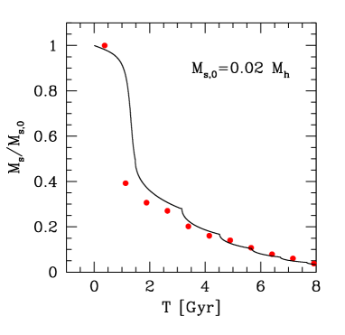
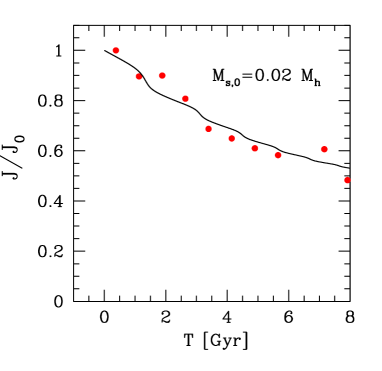
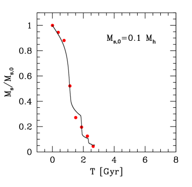
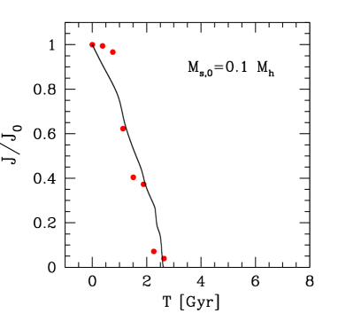
Figure 6: We plot the time evolution of the mass, in units of the initial mass (left panels), and orbital angular momentum scaled to the initial one (right panels). The adopted values are: $M_{\rm s,0}=0.1\,M_{\rm h}$ and $M_{\rm s,0}=0.02\,M_{\rm h}$. The concentration ratio and orbital parameters are $c_{\rm s}/c_{\rm h}=2$, $\epsilon=0.7$ and $x_{\rm c}(E)=0.5$, respectively. Points are from N-body runs and solid line from our semi-analytical model.

In Fig. (5) we show the evolution of a satellite with mass $M_{\rm s,0}=0.01M_{\rm h}$; the orbital parameters are chosen to reflect a typical cosmological orbit: $\epsilon=0.65$ and $x_{\rm c}(E)=0.5$. The bottom panel shows a low $c_{\rm s}/c_{\rm h}$ satellite, disrupted after the second passage to pericenter. The top panel shows the evolution of a higher $c_{\rm s}/c_{\rm h}$ satellite surviving for more than 12 Gyr, despite having lost more than the 99 per cent of its mass. Until the first pericenter passage only the tidal cut accounts for the mass loss. The good agreement between the simulation and the code before the first pericenter passage suggests that the TB recipe is accurate enough to reproduce the mass loss before (or in absence of) the shock heating.

5.4.2 The combined effect of dynamical friction and tidal stripping

The dynamical evolution of a satellite is driven by the combined effect of dynamical friction that drives the satellite to the center of the main halo, and the tidal perturbation which reduces its mass. The two processes are intimately connected as the drag force is strongly related to the mass and size of the satellite.

In Fig. (6) we compare the semi-analytical model with the the results of N-body simulations for satellites with $c_{\rm s}/c_{\rm h}=2$. The initial orbital parameters are $\epsilon=0.7$, and $x_{\rm c}(E)=0.5$. We study two different cases: a light satellite of mass $M_{\rm s,0}=0.02\,M_{\rm h}$ and a massive one with $M_{\rm s}=0.1\,M_{\rm h}$. The mass loss rate and the orbital evolution are well reproduced in both cases. The massive satellite loses mass during evolution, yet a core of bound particles survives having 5% of its initial mass but sinks to the center merging with the main halo in 3 orbital periods. On the contrary, the light satellite loses 99% of its mass but a bound core remains which moves on an inner orbit stable against dynamical friction, following mass loss.

6 The fate of satellites

6.1 The recipe

We now use our semi-analytical model to quantify how mass loss affects the orbital decay. In Fig. (7) we give as a function of $M_{\rm s,0}/M_{\rm h},$ the ratio of the dynamical friction time of a rigid satellite $\tau_{\rm df,rig}$ to the same time for a homologous live satellite $\tau_{\rm df,live}$ . In taking the ratio we mainly quantify the importance of mass loss in affecting the lifetime of a satellite. Fig. (7) shows that massive satellites ($M_{\rm s,0}/M_{\rm h}>0.1$) sink to the center of the main halo on a timescale $\tau_{\rm df,life}\sim\tau_{\rm df,rig}$ as if they were rigid.

Figure 7: We have plotted the ratio of the dynamical friction time of a non-deformable satellites to the same time for a live satellite of equal mass, initially, as function of $M_{\rm s,0}/M_{\rm h}$. The concentration ratio is $c_{\rm s}/c_{\rm h}=2,$ and $x_{\rm c}(E)=0.5.$ We vary the circularity which is labeled with different symbols. We notice that symbols for $\epsilon=0.3$ refer to a different orbital energy: $x_{\rm c}(E)=0.3.$

In the mass range $M_{\rm s,0}\simeq 0.005-0.1M_{\rm h}$ the satellites sink toward the center of the main halo by dynamical friction and so lose mass efficiently. Accordingly, the dynamical friction time $\tau_{\rm df,live}$ is a few to several times longer than $\tau_{\rm df,rig}.$ At lower masses, $M_{\rm s,0}\sim<0.005\,M_{\rm h},$ orbits are less perturbed by friction and mass stripping becomes less important. Thus the ratio $\tau_{\rm df,rig}/\tau_{\rm df,life}$ starts to rise again.

We now estimate the dynamical friction timescale for a live satellite in three different regimes.

For massive satellites, $M_{\rm s,0}\geq 0.1\;M_{\rm h}$, the dynamical friction time is not affected by the mass loss so

$$\tau_{\rm df,live}\sim\tau_{\rm df,rig}\simeq 0.5\>{R^{2}_{\rm h}V_{\rm h}\over GM_{\rm s}}\>{\cal A}_{\rm rig}\left[{M_{\rm s,0}\over M_{\rm h}},c_{\rm h},x_{\rm c}(E)\right]\;,$$ (24)

where:

$${\cal A}_{\rm rig}\left[{M_{\rm s,0}\over M_{\rm h}},c_{\rm h},x_{\rm c}(E)\right]=f(c_{\rm h})\,{x_{\rm c}^{1.97}(E)\over\ln\left(1+{M_{\rm h}/M_{\rm s,0}}\right)}\;,$$ (25)

and $f(c_{\rm h})$ is given by equation (13). In this case, the dynamical friction time depends weakly on $\epsilon$; the exponent $\alpha\approx 0$, as indicated by equation (4). For ${0.007\;M_{\rm h}<M_{\rm s,0}<0.08\;M_{\rm h}}$, we provide a fit of the form:

$$\tau_{\rm df,live}\sim{R_{\rm h}^{2}\;V_{\rm h}\over{GM_{\rm s,0}}}{\cal A}_{\rm live}\left[{M_{\rm s,0}\over M_{\rm h}},\frac{c_{\rm s}}{c_{\rm h}},x_{\rm c}(E),\epsilon\right]\;.$$ (26)

For $\epsilon=1$

$${\cal A}_{\rm live}\left({M_{\rm s,0}\over M_{\rm h}},\frac{c_{\rm s}}{c_{\rm h}},x_{\rm c},\epsilon=1\right)=\left[{0.25\over(c_{\rm s}/c_{\rm h})^{6}}-0.07\,\frac{c_{\rm s}}{c_{\rm h}}+1.123\right]$$

$$~{}~{}~{}~{}~{}~{}~{}~{}~{}~{}~{}~{}~{}~{}~{}\times\left[B(x_{\rm c})\left({M_{\rm s,0}\over M_{\rm h}}\right)^{0.12}+C(x_{\rm c})\left({M_{\rm s,0}\over M_{\rm h}}\right)^{2}\right]\;,$$ (27)

where

$$B(x_{\rm c})=-0.050+0.335\,x_{\rm c}+0.328\,x_{\rm c}^{2}\;,$$ (28)

$$C(x_{\rm c})=2.151-14.176\,x_{\rm c}+27.383\,x_{\rm c}^{2}\;.$$ (29)

This fit reproduces the semi-analytic estimate of the decay time of a live satellite on circular orbits with an error of $\gse 9$ per cent, for $0.2<x_{\rm c}(E)<1$.

Figure 8: The dynamical friction time of life satellites As function of the satellite initial mass. Symbols are the results obtained from the semi-analytic code, lines are the prescription of the fitting formulae (from equation [27] to equation [32]). We set the circularity $\epsilon=0.7$ and the relative concentration $c_{\rm s}/c_{\rm h}=2$ and we vary the orbital energy: $x_{\rm c}(E)=0.5$ (solid line and squares), $x_{\rm c}(E)=0.7$ (dotted line and stars), $x_{\rm c}(E)=0.3$ (dashed line and circles).

For eccentric orbits we find that:

$${\cal A}_{\rm live}\left({M_{\rm s,0}\over M_{\rm h}},\frac{c_{\rm s}}{c_{\rm h}},x_{\rm c},\epsilon\right)={\cal A}_{\rm live}\left({M_{\rm s,0}\over M_{\rm h}},\frac{c_{\rm s}}{c_{\rm h}},x_{\rm c},\epsilon=1\right)\,$$

$$\times\left[0.4+{\cal Q}\left({M_{\rm s,0}\over M_{\rm h}},x_{\rm c}\right)\times(\epsilon-0.2)\right]\;,$$ (30)

where

$${\cal Q}\left({M_{\rm s,0}\over M_{\rm h}},x_{\rm c}\right)=0.9+10^{8}\left(12.84+3.04\,x_{\rm c}-23.4\,x^{2}_{\rm c}\right)$$

$$\times\left({M_{\rm s,0}\over M_{\rm h}}-{0.0077\over 1-1.08x_{\rm c}}-0.0362\right)^{6}$$ (31)

This formula holds when $0.3<x_{\rm c}<0.9$ and $0.3<\epsilon<0.8$ and reproduces the semi-analytical data within and error of $15\%$.

Interestingly, we notice that for an eccentric orbit the decay time can be longer that the DF  time on the circular orbit with the same initial orbital energy, since mass loss on eccentric orbit is higher because of the tidal shock.

For $\epsilon>0.8,$ ${\cal{A}}_{\rm live}$ we use the interpolation of equations (31) and (28). If ${0.08\;M_{\rm h}<M_{\rm s,0}<0.1\;M_{\rm h}}$, we suggest to linear interpolate equations (25) and (27).

Satellites $M_{\rm s,0}\lse 0.007\;M_{\rm h}$, evolve on slightly perturbed orbits, the dynamical friction timescale in this case is al least two times longer than for the rigid satellite (CMG99 similarly found an increase of a factor $e$ for $M_{\rm s,0}=0.02M_{\rm h}$). We suggest to use equation (12) for $\tau_{\rm{df,life}},$ in this mass range, increased by a factor $\sim 2.73$, together with equation (15) for the exponent $\alpha,$ to account for the correction to circularity. For very light satellites ($M_{\rm s,0}<10^{-4}M_{\rm h}$) equation (14) holds.

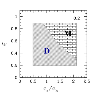
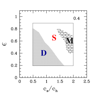
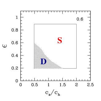
Figure 9: The life diagram of a satellite with $M_{\rm s,0}=0.01\,M_{\rm h}$. Each plot is labeled with the value of the $x_{\rm c}(E)$. We identify the region of the parameters space where the satellite sinks to the center of the main halo (M), evaporates in the background (D) or survives (S).

In Appendix B we give a simple expression for the disruption time $t_{\rm dis}$ that can be used for a comparison with the other timescale.

6.2 Merging, distruption or survival

We here investigate the dynamical evolution of a population of satellites, in a given halo. An individual satellite is labeled by four parameters; $x_{\rm c}(E)$ and $\epsilon$ identify the orbit, while initial mass $M_{\rm s,0}$ and concentration $c_{\rm s}$ identify the internal properties. Each combination of the four parameters leads to a different final state for the satellite: rapid merging toward the center of the main halo (M), disruption (D), or survival (S) (when a residual mass $M_{\rm s}$ remains bound and maintains its identity, orbiting in the main halo for a time longer than the Hubble time).

An important role is played by the concentration ratio as shown by the life diagrams in Fig. (9). These predict the final fate of a satellite with $M_{\rm s,0}=0.01\,M_{\rm h}$, as function of the $c_{\rm s}/c_{\rm h}$ and of the orbital parameters. The fractional area in this parameter space leading to disruption, survival or decay is an estimate of the relative importance of these processes in determining the satellite fate. Disruption due to the tidal perturbation is the fate of those satellites that initially move on close orbits despite $c_{\rm s}/c_{\rm h}.$ Satellites moving along typical (plunging) cosmological orbits survive over a Hubble time only if they had a concentration higher than that of the main halo at the time of their infall.

Figure 10: Probability distribution for the three final endpoints: merging (M), disruption (D) or survival (S) as function of the initial satellite mass. The thick solid line refers to the case of a rigid satellite.

In Fig. (10) we have drawn the probability distribution relative to the three final states: direct merging (by dynamical friction), which dominates at large masses, survival and/or disruption which is the most likely end for satellite with $M_{\rm s,0}<0.01\,M_{\rm h}.$ In producing Fig. (10) we have generated evolutionary paths (ending after a time equal to the Hubble time) for satellites starting from a flat distribution of orbital parameters and concentrations.

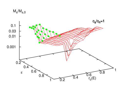
Figure 11: The mass that remains as a function of the orbital parameters after more than a Hubble time, for a satellite with $M_{\rm s,0}=0.01\,M_{\rm h}.$ Dots identify the regions where the satellite is disrupted. The contour line on the xy plane identify the loci where $M_{\rm s}/M_{\rm s,0}=0.1$.

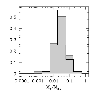
Figure 12: The distribution of the final mass of a satellite of initial mass $M_{\rm s}=0.01M_{\rm h}$ after more than a Hubble time. Histograms are derived starting from a uniform distribution of orbital parameters, for two values of the concentration ratio: $c_{\rm s}/c_{\rm h}=2$ (filled grey area) and $c_{\rm s}/c_{\rm h}=1$.

Our study suggests that those satellites that survive have lost memory of their initial state: dynamical friction perturbs the orbit and tidal stripping reduces the satellite mass. In Fig. (11) we compute the mass of the satellites that remains after a Hubble time. The figure refers to a high concentration case, but we extend our analysis also to low concentrated satellites as shown in Fig. (12), where we compute the cumulative mass distribution for all the initial orbital parameters. On average, much less then 10% of the initial mass remains bound. Of course, in general circular orbits do not cause serious damages to the satellite as shock heating is less intense (an exception is represented by satellites on very tightly bound orbits). In Fig. (11), dots show the final mass just prior evaporation. As expected, radial orbits can more easily dissolve a satellite.

The strength of the orbital decay can be estimated measuring the reduction of the apocenter distance.

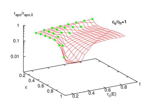
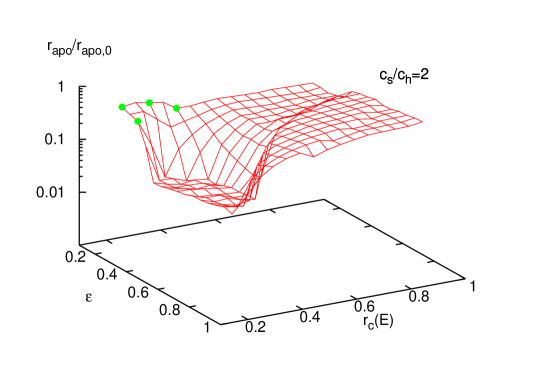
Figure 13: The apocenters radius in units of its initial value for a satellite $M_{\rm s,0}=0.01M_{\rm h}$ evaluated after more than a Hubble time (we terminate at $15$ Gyr). The two plots refer to $c_{\rm s}/c_{\rm h}=2$ (bottom) and $c_{\rm s}/c_{\rm h}=1$ (top). Dots identify satellites that evaporate before 15 Gyr. The contour lines on the xy plane select the regions where the relative reduction of $r_{\rm apo}$ is 0.1 (dotted lines) and 0.5 (dashed lines).

In Fig. (13) we plot the distribution of apocenter radii for a satellite with $M_{\rm s,0}=0.01M_{\rm h}$ after 15 Gyr of orbital evolution. The strength of the drag force reduces the apocenter distance by a factor of two for cosmological orbits and it is not significantly affected by the concentration.

6.3 Cosmological examples

Now, we apply our analysis to some cosmological relevant examples. We discuss the evolution of different satellites which orbit in a cluster-like and galaxy-like haloes. The cluster halo is a Coma-like cluster with mass $M_{\rm h}=5\cdot 10^{15}M_{\odot}$ and concentration $c_{\rm h}=3.44$. The Milky Way-like galaxy halo has $M_{\rm h}=10^{12}M_{\odot}$ and $c_{\rm h}=10.44$. For all cases, the initial orbital parameters are chosen as $\epsilon=0.6$ and $x_{\rm c}(E)=0.5$.

Group in Coma

We consider a massive group-like satellite of mass $M_{\rm s,0}=3\cdot 10^{13}M_{\odot}$ and $c_{\rm s}=7.5$ which enters the Coma-like halo at $z=0.5$. In a $\Lambda$CDM Cosmology it evolves for $\sim$4.8 Gyr inside the halo until $z=0$.

As suggested by the high value of $c_{\rm s}/c_{\rm h}$ the satellite is not disrupted. Since $M_{\rm s,0}=0.006M_{\rm h}$ the orbit is stable and, with this choice of the initial orbital parameters, the satellite evolves for $\sim$ 1.5 P_orb. The final apocenter radius is $r_{\rm apo}\simeq 0.85r_{\rm apo,0}$ and its final mass is $M_{\rm s}=7.2\cdot 10^{12}M_{\odot}$.

Milky Way in Coma

A Milky Way-like satellite has mass $M_{\rm s,0}=10^{12}M_{\odot}$ and $c_{\rm s}=10.44$. If it enters the Coma-like halo at $z=0.5$ it evolves for $\sim$ 1.5 P_orb. The orbit remains almost unperturbed ($r_{\rm apo}\simeq 0.99r_{\rm apo,0}$) as strength of the drag force is extremely weak since $M_{\rm s,0}=0.0002M_{\rm h}$. Due to the extremely high relative concentration, $c_{\rm s}/c_{\rm h}\simeq 3$ the satellite does not evaporate and its final mass ad $z=0$ is $M_{\rm s}=2.5\cdot 10^{11}M_{\odot}$

Large Magellanic Cloud in Milky Way

A Large Magellanic Cloud halo has $M_{\rm s,0}=10^{11}M_{\odot}$ and $c_{\rm s}=11.9$. As expected due to its relative high mass, the satellite merges with the Milky Way in $\sim$ 4 Gyr. Before merging, the satellite loses 97% of its mass that is dispersed in the Milky Way Halo.

Dwarf in Milky Way

We consider a Dwarf-like satellite of mass $M_{\rm s,0}=5\cdot 10^{9}M_{\odot}$ and concentration $c_{\rm s}=13.6$. If it enters the Milky Way-like halo at $z=0.5$ it evolves on an almost unperturbed orbit for $\sim$ 2 P_orb and its final mass is $M_{\rm s}=2\cdot 10^{8}M_{\odot}$.

Dwarf in Milky Way at high redshift A Dwarf-like satellite enters a Milky Way-like halo at $z=2$, when the Milky Way has mass $M_{\rm h}=10^{11}M_{\odot}$ and concentration $c_{\rm h}=6.15$. The satellite has $M_{\rm s,0}=5\cdot 10^{9}M_{\odot}$ and $c_{\rm s}=6.8$. The dwarf evolves for $\sim$11 Gyr. Due to its low relative concentration it loses 99% of its initial mass during the first orbital period; its orbit then becomes stable ($r_{\rm apo}\simeq 0.36r_{\rm apo,0}$). Note that here we are not accounting for the evolution of the main halo which grows in mass during the remaining 11 Gyr before $z=0$, but the influence of accreted mass on the central regions dynamics should be relatively small (Helmi et al 2002) Finally we notice that our Milky Way model does not account for the presence of a disk. Penarrubia, Kroupa & Boily (2002) suggest that orbital evolution changes when the potential well has a flattened component, and DF is more efficient for satellites with low-inclination orbits (respect to the disk): the orbital decay is accelerated and the orbital plane decays over the disk plane. They also find instead that DF enhances the survival time of satellites when they move on near-polar orbits.

7 Summary and Conclusions

We coupled together two successful models for dynamical friction and tidal stripping and compared their predictions with high resolution N–body simulations to address the evolution and ultimate fate of satellite haloes within cosmic structures. Under the assumption that haloes are well described by an NFW profile we are able to predict if a satellite of given mass, orbital eccentricity and infall redshift, will merge, evaporate or survive under the simultaneous action of dynamical friction and tidal mass loss.

We emphasize that we have obtained a complete predictive scheme for the fate of a satellites whose masses at the time of infall into the main halo are known (below we refer to typical cosmological orbits):

• High mass satellites ($M_{\rm s,0}>0.1M_{\rm h}$) sink rapidly toward the center of the main halo without significant mass dispersal: The dynamical friction timescale for a rigid satellite (equation [24]) gives the correct timescale of merging.

• For satellites of mass $0.01M_{\rm h}<M_{\rm s,0}<0.1M_{\rm h}$ dynamical friction is still strong and drives the satellite toward the center where tidal mass loss become severe. Low concentration satellites are disrupted, while high concentration satellites, severely pruned by the tidal field, survive with masses $0.01M_{\rm s,0},$ and settle into inner orbits with a typical reduction of the apocenter radii of a factor $\sim 0.1$ lower relative to the initial value. The dynamical friction timescale for these satellites is longer than for their rigid counterpart, and is given by equation (26).

• Light satellites with mass $M_{\rm s,0}<0.01M_{\rm h}$ are almost unaffected by dynamical friction which is operating on a rather long timescale. Mass loss by the tidal field, which is not severe on these cosmological orbits, stabilizes further the orbit.

• Low concentration satellites below $0.1M_{\rm h}$ can be disrupted by tides before their orbital decay is complete. Comparison of the dynamical friction timescale and the disruption timescale as provided in this paper allows to find the actual lifetime of satellite haloes.

We predict that, because of the combined action of stripping and dynamical friction, a primary halo at $z=0$ will host preferentially satellites with mass $M_{\rm s}/M_{\rm h}\ll 0.01$ as the heavier ones would have been accreted or/and dispersed in the background, leaving a “depression” in the mass function of substructure above 0.01 $M_{\rm s}/M_{\rm h},$(of course we are neglecting effects due to the evolution of the main halo itself). This feature should be more evident in Milky Way-size haloes than in cluster haloes as in the former bound satellites had more time to evolve.

Since the destructive power of the tidal field (and in particular of tidal shocks) depends sensitively on the degree of circularity of the satellite orbit, a large galaxy halo like that of the Milky Way ($>10^{12}M_{\odot}$) should host satellites moving preferentially on circular orbits as a consequence of the selective action of the tidal field. Also, because dynamical friction seems unable to render the satellites’ orbit circular (van den Bosch et al. 1999; CMG99), the low eccentricities should have been already present as initial conditions. This “selection effect” will be extremely weak for smaller satellites (below $0.01-0.001M_{\odot}$) because their orbit barely decays and thus will have in general long survival times (only low concentration satellites could disappear quickly but they are not common in CDM models; see e.g. Eke, Navarro & Steinmetz 2001 and Bullock et al.2001). This mass regime corresponds to that of the dwarf spheroidal satellites of the Milky Way. On the other end, the Magellanic Clouds, the dwarf elliptical satellites of M31 and perhaps the dwarf spheroidal Fornax are all massive enough to fit in the intermediate regime where destruction is still possible; thus these galaxies could have survived because their host haloes had nearly circular orbits. In the case of the Magellanic Clouds a nearly circular orbit is indeed measured (Kroupa & Bastian 1999). There is, however, at least one caveat to this interpretation, namely that both the dwarf ellipticals of M31 and the Magellanic Clouds could be dense enough to survive shocks on even very eccentric orbits (Mayer et al. 2001b). Only when all the orbits of the satellites will be accurately determined we will know whether eccentricity or internal structure was more important in determining their survival.

The calculations described in this paper can become a useful tool when coupled to cosmological simulations. The final goal is to find an appropriate description of the dynamical evolution of substructure in a halo. Increasing computing power and code performances has recently allowed to carry out extremely high resolution simulations that follow the evolution of substructure in dark matter haloes (Ghigna et al. 1998, 2000; Mayer et al. in preparation). These represent the new ground where CDM models are being tested and their predictions compared to observations. However, these simulations remain costly and usually only one system at a time can be simulated down to very small scales. On the other end, resolving the mass function of substructure in depth is important in light of the problem of the overabundance of satellites (Moore et al. 1999; Klypin et al. 1999). Such mass function can be viewed as the convolution of the mass function of satellites at an earlier epoch with an evolutionary filter function that depends on the dynamical mechanisms analyzed in this work. Therefore, our results can allow to address the substructure problem in a statistical way orders of magnitude faster than with N-Body simulations; as an example one can explore a large number of dynamical histories by randomly varying the orbital and structural parameters in the range typical of cold dark matter cosmogonies, and work is in progress (Taffoni et al. 2002 in prep). Here we make a first attempt starting with uniform distributions. Clearly the time dependent potential of the growing primary halo, whether it is a galaxy or a cluster, is an additional ingredient that only simulations can incorporate and which could affect the orbital dynamics of the satellites. However, the latter limitation can be partially overcome by using the merger tree extracted from a low resolution simulation, as done within some semi-analytical models (Somerville & Primack 1999; Kauffmann et al. 1999; Cole et al. 2000) or using analytical merger trees providing a good approximation to the latter (Taffoni et al. 2002; Monaco et al. 2002).

A key result of our analysis, and one that is in agreement with the high resolution cosmological simulations from which the initial orbits were drawn, is that the inner, most bound part of small satellites as concentrated as expected in CDM models (Eke, Navarro & Steinmetz 2001; Bullock et al. 2001) survive for timescales comparable to or longer than the age of the Universe. This residual has a size corresponding to a few percents of the initial virial radius; this is comparable to the scale of the baryonic component in galaxies, so we can argue that galaxies will mostly survive within the main halo. This result is also confirmed by high-resolution SPH simulations of the formation of Milky Way-like galaxy (Governato et al. 2002). Indeed, dissipation could make the inner part of the haloes even more robust against tides (Navarro & Steinmetz 2000). On the other end, additional tidal shocks occurring during encounters between substructure haloes, i.e. galaxy harassment (Moore et al. 1996, 1998), might have a counteracting effect and could actually increase mass loss. However, detailed simulations of this mechanism have shown that only very fragile, LSB-type galaxies would be severely damaged by harassment (Moore et al. 1999); halo profiles of these galaxies likely correspond to the low concentration satellites studied in this paper (Van den Bosch & Swaters 2001) which we have shown are easily disrupted even by the tides of the primary halo alone. Thus, adding harassment would only accelerate the disruption of a few satellites while not affecting the survival of the majority of them which, in CDM models, have high concentrations. Hence the picture emerging from the life diagrams of the satellites shown in this paper is robust. Satellites close to disruption at the present time, like Sagittarius in the Milky Way subgroup, must have been much bigger in the past in order for dynamical friction to drag them to an inner orbit where dissolution can easily take place; alternatively they could have entered the halo at fairly high redshift, which would place them naturally on an inner, tightly bound orbit (Mayer et al. 2001b). In clusters, dwarf galaxies cannibalized by giant CD galaxies might also trace an early population.

Satellites infalling at redshift one or lower in the main haloes will complete several orbits and eventually undergo morphological changes by tidal stirring (Mayer et al. 2001a,b) and harassment (Moore et al. 1996, 1998). These will produce diffuse streams of stars while they are orbiting (Helmi & White 1999; Johnston, Sigurdsson & Hernquist 1999), contributing to the build up of an extended stellar halo population. Such population should be present out to more than 200 kpc in the Milky Way halo, as the plunging orbits of satellites seen in cosmological simulations go this far out. On the contrary, a less extended stellar halo should be expected if dynamical friction were more efficient in dragging satellites to the center. The amount of stellar halo substructure out to large distances could thus reveal the original mass function of observed dwarf spheroidal galaxies in the Local Group. Components decoupled in their kinematics as well as in the metallicity and age of their stars should be present, but tracking such properties might be a daunting task observationally if enough phase mixing occurs (Ibata et al. 2001a,b); however, while in the inner halo fast orbital precession and heating by other clumps might blur the streams, the phase space distribution of the outer halo material should still carry the memory of the initial orbits of the satellites (Mayer et al. 2002).

The prescriptions for the decay and disruption rates obtained in this work provide a complete framework which can improve the predictive power of semi-analytical models of galaxy formation. They enable to follow the complex evolution of substructures in hierarchical models in a straightforward manner.

8 Acknowledgments

The authors like to thank Tom Quinn and Joachim Stadel for providing us PKDGRAV. Thanks go to Marta Volonteri and Pierluigi Monaco for useful discussions and to Valentina D’odorico for the critical reading of the manuscript. Simulations have been carried out at the CINECA Supercomputing Center (Bologna) and on a dual-processor ALPHA workstation at the University of Washington. L. Mayer was supported by the National Science Foundation (NSF Grant 9973209).

Appendix A Calculation of the tidal energy for a NFW profile

At each pericenter passage the satellite crosses very rapidly the central and more concentrated regions of the primary halo. The duration of those encounters is fast compared with the dynamical time of the object. Such kind of interactions are called tidal shocks (Spitzer 1987). We will use the results derived by GHO to describe the amount of heating due to tidal shocks on a satellite moving inside an extended mass distribution.

During an orbital period $P_{\rm orb}$ the tidal force $\mathbf{f}_{\rm s,tid}$ per unit mass produces a global variation on the velocity of the internal fluid:

$$\Delta{\bf v}=\int_{0}^{P_{\rm orb}}{\bf f}_{\rm tid}\;dt\;,$$ (32)

where we have applied the impulse approximation in the hypothesis that the time scale of interaction is short compared with the dynamical time of the satellite ($t=0$ refers to the initial satellite position at apocenter distance).

In a spherically symmetric system of mass $M_{\rm h}$, the tidal force per unit mass exerted by the background on a dark matter particle of the satellite is:

$${\bf f}_{\rm tid}=\frac{GM_{\rm h}}{R_{\rm h}^{3}}[(3\mu-\mu^{\prime})(\hat{\bf r}\cdot{\bf R_{\rm s}})\hat{\bf r}-\mu{\bf R_{\rm s}}]\;,$$ (33)

where $\hat{\bf r}={\bf r}/R_{\rm h}$ is the direction to the center of mass of the satellite (CMS), $\mathbf{R}_{\rm s}$ is the position of the particle respect to CMS. Note that $R_{\rm h}$ is the virial radius of the main system. Here:

$$\mu(r)=\frac{M(r)}{M_{\rm h}}$$ (34)

is the adimensional mass profile, and:

$$\mu^{\prime}(r)=\frac{d\mu(r)}{d\ln r}\;.$$ (35)

For a NFW profile $\mu$ and $\mu^{\prime}$ are functions of the normalized radius $x=r/R_{\rm h}$ and of the concentration $c_{\rm h}$ of the primary halo:

$$\mu(x,c_{\rm h})={\ln(1+c_{\rm h}x)-c_{\rm h}x/(1+c_{\rm h}x)\over\ln(1+c_{\rm h})-c_{\rm h}/(1+c_{\rm h})}\;,$$ (36)

and

$$\mu^{\prime}(x,c_{\rm h})={1\over\ln(1+c_{\rm h})-c_{\rm h}/(1+c_{\rm h})}\left({c_{\rm h}x\over 1+c_{\rm h}x}\right)^{2}\;.$$ (37)

In the case of stable orbits the angular momentum $J$ is conserved and we can use the identity

$$dt=(r^{2}/J)d\theta$$ (38)

to re-write equation(32) into components (GHO):

$$\Delta{\bf v}={GM_{\rm h}\over rJ}\{(B_{1}-B_{3})x,(B_{2}-B_{3})y,-B_{3}z\}\;,$$ (39)

where

$$B_{1}(c_{\rm h}) = \int_{-\theta_{m}}^{-\theta_{m}}\,F_{1}(x,c_{\rm h})\,\cos^{2}{\theta}\,d\theta$$ (40)

$$B_{2}(c_{\rm h}) = \int_{-\theta_{m}}^{-\theta_{m}}\,F_{1}(x,c_{\rm h})\,\sin^{2}{\theta}\,d\theta$$ (41)

$$B_{3}(c_{\rm h}) = \int_{-\theta_{m}}^{-\theta_{m}}\,{\mu(x,c_{\rm h})\over x}\,d\theta,$$ (42)

where $\theta_{m}$ is the maximum value of the position angle, and:

$$F_{1}(x,c_{\rm h})=3$$

$$\times{[\ln(1+c_{\rm h}x)-c_{\rm h}x/(1+c_{\rm h}x)]-[c_{\rm h}x/(1+c_{\rm h}x)]^{2}\over x[\ln(1+c_{\rm h})-c_{\rm h}/(1+c_{\rm h})]}\;.$$ (43)

This velocity changes cause a reduction of the binding energy of the system:

$$\langle\Delta E\rangle=\left\langle\frac{1}{2}|\Delta{\bf v}|^{2}\right\rangle\;.$$ (44)

Averaging over an ensemble of dark matter particles in a spherically symmetric satellite we have that $\langle x^{2}\rangle=\langle y^{2}\rangle=\langle z^{2}\rangle=R_{\rm s}^{2}\>/\>2$, and using equation(39), the tidal energy gained by the satellite becomes:

$$\langle\Delta E\rangle = \left({GM_{\rm h}\over J\,R_{\rm h}}\right)^{2}$$ (45)

$$\times \left[{(B_{1}-B_{3})^{2}+(B_{2}-B_{3})^{2}+B_{3}^{2}\over 6}\right]\;R_{\rm s}^{2}\;.$$

In the previous expression, the contribution due to the halo and the orbital parameters ($\epsilon$ and $x_{c}^{2}[E]$) is confined in the function:

$$\Xi\left[c_{\rm h},x_{\rm c}(E),\epsilon\right] = \left({GM_{\rm h}\over R_{\rm h}^{2}V_{\rm h}}\right)^{2}{1\over x_{\rm c}^{2}(E)\,\epsilon^{2}}$$ (46)

$$\times \left[{(B_{1}-B_{3})^{2}+(B_{2}-B_{3})^{2}+B_{3}^{2}\over 6}\right]\;,$$

here $V_{\rm h}$ is the circular velocity of the main halo at virial radius.

It is then useful to write the shock energy as:

$$\langle\Delta E\rangle=\Xi\left[c_{\rm h},x_{\rm c}(E),\epsilon\right]\;R_{\rm s}^{2}\;.$$ (47)

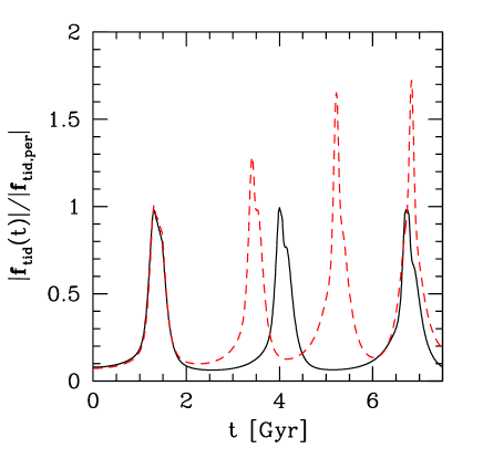
Figure 14: The intensity of the tidal force $|{\bf f}_{\rm tid}(t)|$ normalised to its value at the first periastron $|{\bf f}_{\rm tid,per}|$. We plot the module of the tidal force (equation [33]) as a function of time for a satellite of mass $M_{\rm s,0}=0.01M_{\rm h}$ and $\epsilon=0.7$ $x_{\rm c}(E)=0.5$. The solid line refers to a stable orbit, the dashed line to an unstable one. When the drag force is active, the intensity of the tidal force, and consequently of the shock energy, grows with time.

When the frictional drag force is active, it is not possible to change the integration variable according to equation (38). The energy change becomes:

$$\langle\Delta E\rangle = \left({GM_{\rm h}\over R_{\rm h}^{3}}\right)^{2}$$

$$\times \left[{(A_{1}-A_{3})^{2}+(A_{2}-A_{3})^{2}+A_{3}^{2}\over 6}\right]\;R_{\rm s}^{2}\;.$$ (48)

Here

$$A_{1}(\epsilon,x_{\rm c}[E]) = \int_{0}^{P_{\rm orb}}\,F_{2}(x,c_{\rm h})\,\cos^{2}{\theta}\,dt$$ (49)

$$A_{2}(\epsilon,x_{\rm c}[E]) = \int_{0}^{P_{\rm orb}}\,F_{2}(x,c_{\rm h})\,\sin^{2}{\theta}\,dt$$ (50)

$$A_{3}(\epsilon,x_{\rm c}[E]) = \int_{0}^{P_{\rm orb}}\,{\mu(x,c_{\rm h})\over x^{3}}\,dt,$$ (51)

with

$$F_{2}(x,c_{\rm h})={F_{1}(x,c_{\rm h})\over x^{2}}$$ (52)

Once again we separate the contribution due to the environment:

$${\cal F}[c_{\rm h},x_{\rm c}(E),\epsilon] = \left({GM_{\rm h}\over R_{\rm h}^{3}}\right)^{2}$$ (53)

$$\times \left[{(A_{1}-A_{3})^{2}+(A_{2}-A_{3})^{2}+A_{3}^{2}\over 6}\right]\;.$$

For an unstable orbit

$$\langle\Delta E\rangle={\cal F}\left[c_{\rm h},x_{\rm c}(E),\epsilon\right]\;R_{\rm s}^{2}\;.$$ (54)

The shock energy in this case must be evaluated along the perturbed orbit. As the drag force drives the satellite in the internal region of the halo the $\langle\Delta E\rangle$ increases (Fig. [14]).

Appendix B An approximate estimate of the disruption timescale

Because the lifetime of light satellites is mostly set by tidal disruption we estimate here the disruption time. If the main halo density profile is isothermal (ISO) then GHO showed that the shock energy change is:

$$\langle\Delta E\rangle_{\rm ISO}=\left(V_{\rm h}\over R_{\rm h}\right)^{2}{2\sin^{2}\theta_{\rm m}+4\theta^{2}_{\rm m}\over 6(\epsilon\;x_{\rm c})^{2}}A(x_{\tau})\cdot R_{\rm s}^{2}\;,$$ (55)

where $\theta_{\rm m}$ is the maximum value of the position angle which varies from $\pi/2$ to $\pi$. Using the orbit equation (equation [6]) we can evaluate $\theta_{\rm m}$:

$$\theta_{\rm m}=2\,\epsilon\,x_{\rm c}\int_{r_{\rm per}}^{r_{\rm apo}}{dx\over x^{2}\sqrt{\ln(r_{c}/x)^{2}-(r_{c}/x)^{2}\epsilon^{2}-1}}$$ (56)

and the orbital period

$$P_{\rm orb}=2{R_{\rm h}\over V_{\rm h}}\,\int_{r_{\rm per}}^{r_{\rm apo}}{dx\over\sqrt{\ln(r_{c}/x)^{2}-(r_{c}/x)^{2}\epsilon^{2}-1}}\;.$$ (57)

The shock in the ISO profile equals the shock of an NFW case when $c_{\rm h}=30$. We have than:

$$\langle\Delta E\rangle_{\rm NFW}\sim\langle\Delta E\rangle_{\rm ISO}\times(0.029\;c_{\rm h}+0.13)\;.$$ (58)

At each pericenter passage the satellite is shock heated and its radius $R_{\rm s}$ is reduced of a factor $\Delta R$. As an approximation $\Delta R\sim R_{\rm s,0}/N$ where $N$ is the number of pericenter passages necessary to destroy the satellite. Then, we have an implicit equation for $N$

$$N+\frac{1}{N}\sum_{i=1}^{N-1}i^{2}={E_{0}\over\langle\Delta E\rangle_{\rm NFW,0}}\;,$$ (59)

where $E_{0}=0.5GM_{\rm s}/R_{\rm s,0}$, and $\langle\Delta E\rangle_{\rm NFW,0}$ is evaluated at the initial half mass radius. Since

$$\sum_{i=1}^{N-1}i^{2}={N\,(N-1)\,(2N-1)\over 6}$$ (60)

for large N equation (59) would give:

$$N\approx\sqrt{48{E_{0}\over\langle\Delta E\rangle_{\rm NFW,0}}}\;.$$ (61)

The disruption time can then be written as:

$$t_{\rm dis}\sim P_{\rm orb}\cdot N\;.$$ (62)

This formula provides a simple estimate of the disruption time valid on cosmological relevant orbits with a precision of 25 per cent.

References

- [1] Binney, J., & Tremaine, S. 1987, Galactic Dynamics (Princeton: Princeton Univ. Press)
- [2] Bullock, J. S.; Kolatt, T. S.; Sigad, Y.; et al., 2001, MNRAS, 321, 559
- [3] Bullock, J. S.; Kolatt, T. S.; Sigad, Y.; et al., 2000, astro-ph/0010222
- [4] Chandrasekhar, S. 1943, ApJ, 97, 255
- [5] Cole S., Lacey C. G., Baugh C. M., Frenk C. S., 2000, MNRAS, 319, 168
- [6] Colpi, M., 1998, ApJ,502,167
- [7] Colpi, M., Pallavicini, A., 1998, ApJ, 502, 150
- [8] Colpi, M., Mayer, L., Governato, F., 1999, ApJ, 525, 720
- [9] Eke, V. R., Navarro, J. F., Steinmetz, M., 2001, ApJ, 554, 114
- [10] Fukushige, T., & Makino, J., 2001, ApJ, 557, 533
- [11] Ghigna, S,, Moore, B., Governato, F., Lake, G., Quinn, T., Stadel, J. 1998, MNRAS, 300, 146
- [12] Ghigna, S.; Moore, B.; Governato, F.; Lake, G.; Quinn, T.; Stadel, J., 2000, ApJ, 544, 616
- [13] Gnedin, O. Y., Hernquist, L., & Ostriker, J. P. 1999, ApJ, 514, 109;
- [14] Gnedin, O. Y., Lee, H. M., & Ostriker, J. P. 1999, ApJ, 522, 935
- [15] Gnedin, O. Y., & Ostriker, J. P. 1997, ApJ, 474, 223;
- [16] Gnedin, O. Y., & Ostriker, J. P. 1999, ApJ, 513, 626;
- [17] Governato, F., Babul, A., Quinn, T., Tozzi, P., Baugh, C. M., Katz, N., Lake, G., 1999, MNRAS, 307, 949
- [18] Governato, F., Mayer, L., Wadsley, J., Gardner, J., P., Willman, B., Hayashi, E., Quinn, T., Stadel, J., Lake, G., astro-ph/0207044
- [19] Hayashi, E., Navarro, F. J., Taylor, J. E., Stadel, J., Quinn T., astro-ph/0203004
- [20] Helmi, A., White, S. D. M., 1999, MNRAS, 307, 495
- [21] Helmi, A., White, S. D. M., Springel, V., 2002, Phys.RevD, in press, astro-ph/0201289
- [22] Hernquist, L., Weinberg, M. D. 1999, MNRAS, 238, 407
- [23] Huang, S., & Carlberg, R., G., 1997, ApJ, 480, 503
- [24] Ibata, R., Irwin, M., Lewis, G., Ferguson, A., M., N., Tanvir, N., 2001, Nature, 412, 49
- [25] Ibata, R., Lewis, G., F., Irwin, M., Totten, E., Quinn, T., 2001, ApJ, 551, 294
- [26] Jing, Y. P., Suto, Y., 2000, ApJ, 529L, 69
- [27] Johnston, K. V., Sigurdsson, S., Hernquist, L., 1999, MNRAS 302, 771
- [28] Kauffmann, G., White, S. D. M., Guiderdoni, B. 1993, MNRAS, 264, 201
- [29] Kauffmann, G., Colberg, J. M., Diaferio, A., White, S.D.M., 1999, MNRAS, 303, 188
- [30] Klypin, A., Kravtsov, A. V., Valenzuela, O., Prada, F., 1999, ApJ, 522, 82
- [31] Kroupa, P., Bastian, U., 1997, New Astronomy, 2, 77
- [32] Lacey, C., Cole, S. 1993, MNRAS, 262, 627
- [33] Lewis, G. F., Babul, A., Katz, N., Quinn, T., Hernquist, L., Weinberg, D. H., 2000, ApJ, 536, 623
- [34] Mayer, L., Governato, F., Colpi, M., Moore, B., Quinn, T., Wadsley, J., Stadel, J., Lake, G., 2001a, ApJ, 547, L123
- [35] Mayer, L., Governato, F., Colpi, M., Moore, B., Quinn, T., Wadsley, J., Stadel, J., Lake, G., 2001b, ApJ, 559, 754
- [36] Mayer, L., Moore, B., Quinn, T., Governato, F., & Stadel, J., 2002, MNRAS, 336, 119M
- [37] Monaco, P., Theuns, T., Taffoni, G., Governato, F., Quinn, T., Stadel, J., 2002, ApJ, 564, 8
- [38] Moore, B., Katz, N., Lake, G., Dressler, A., & Oemler, A., Jr, 1996, Nature, 379, 613
- [39] Moore, B., Lake, G., Katz, N. 1998, MNRAS, 495, 139
- [40] Moore, B., Lake, G., Quinn, T., & Stadel, J. 1999, MNRAS, 304, 465
- [41] Moore, B., Ghigna, S., Governato, F., Lake, G., Quinn, T., Stadel, J ., Tozzi, P., 1999, ApJ, 524, 19
- [42] Naab, T., Burkert, A., Hernquist, L., 1999, ApJ, 523, 133
- [43] Navarro, J. F., Frenk, C. S., White, S. D. M., 1996, ApJ, 462, 563
- [44] Navarro, J. F., Frenk, C. S., White, S. D. M., 1997, ApJ, 490, 493
- [45] Navarro, J. F., Steinmetz, M., 2000, ApJ, 528, 607
- [46] Ostriker, J. P., Spitzer, L. J., Chevalier, R. A., 1972, ApJ, 176, 51
- [47] Penarrubia J., Kroupa P., Boily C. M., 2002, MNRAS, 333, 779
- [48] Sheth R. K., Lemson G., 1999, MNRAS, 304, 767
- [49] Somerville, R. S., Kolatt, T. S. 1999, MNRAS, 305, 1
- [50] Somerville, R. S., Primack, J. R. 1999, MNRAS, 310, 1087
- [51] Spitzer, L. Jr. 1987, Dynamical Evolution of Globular Clusters (Princeton: Princeton Univ. Press)
- [52] Stadel J., 2002, PhD Thesis, UNIVERSITY OF WASHINGTON, Source DAI-B 62/08, p. 3657
- [53] Taffoni, G., Monaco, P., Theuns, T., 2002, MNRAS, 333, 623
- [54] Taylor, J., Babul, A., 2001, ApJ, 559, 735
- [55] Tormen, G. 1997 , MNRAS, 290, 411
- [56] Tormen, G., Diaferio, A., Seyer, 1998 , MNRAS, 299, 728
- [57] Van Albada, T.S., 1987, IAUS,127, 291
- [58] van den Bosch, F. C., Lewis, G. F., Lake, G., & Stadel, J. 1999, ApJ, 515, 50
- [59] van den Bosch, F. C., & Swaters, Rob A., MNRAS, 325, 1017
- [60] Velázquez, H., & White, S. D. M., 1999, MNRAS, 304, 254
- [] Weinberg, M. D. 1989, MNRAS, 239, 549
- [61] Weinberg, M. D. 1994, AJ, 108, 1398
- [] Weinberg, M. D. 1995 ApJ, 455, 31
- [] Zhang B., Wyse R.F.G., Stiavelli M., Silk J., 2002, astro-ph/0204025