Lowering Inferred Cluster Magnetic Field Strengths - the radio galaxy contributions

Abstract

We present a detailed examination of the relationship between the magnetic field structures and the variations in Faraday Rotation across PKS 1246$-$410, a radio source in the Centaurus cluster of galaxies, using data from Taylor, Fabian and Allen. We find a significant relationship between the intrinsic position angle of the polarization and the local amount of Faraday Rotation. The most plausible explanation is that most or all of the rotation is local to the source. We suggest that the rotations local to cluster radio galaxies may result from either thermal material mixed with the radio plasma, or from thin skins of warm, ionized gas in pressure balance with the observed galaxy or hot cluster atmospheres. We find that the contribution of any unrelated cluster Rotation Measure variations on scales of 2 $-$ 10 arcsec are less than 25 rad/m²; the standard, although model dependent, derivation of cluster fields would then lead to an upper limit of $\approx 0.4\mu{\rm G}$ on these scales. Inspection of the distributions of Rotation Measure, polarisation angle and total intensity in 3C 75, 3C 465 and Cygnus A also shows source-related Faraday effects in some locations. Many effects can mask the signatures of locally-dominated RMs, so the detection of even isolated correlations can be important, although difficult to quantify statistically. In order to use radio sources such as shown here to derive cluster-wide magnetic fields, as is commonly done, one must first remove the local contributions; this is not possible at present.

1 Introduction

The Faraday Rotation of linearly polarized radiation through a magnetic plasma has been used as a diagnostic of conditions in synchrotron sources since the work by e.g., Burn (1966). When the path length through the plasma and the density of thermal electrons can be reasonably estimated, the observed Faraday Rotation, described by the Rotation Measure (RM) in units of rad/m² can be used to derive a characteristic magnetic field strength. This technique has been applied to clusters of galaxies, leading to estimates of partially disordered cluster-wide fields which vary between less than 1 $\mu{\rm G}$ [e.g. Lawler & Dennison (1982) and Hennessy, Owen & Eilek (1989)] to 1$-$40$\mu{\rm G}$ [e.g. Kim, Tribble & Kronberg (1991), Ge & Owen (1993), Feretti et al (1999), Clarke, Kronberg & Böhringer (2001), Taylor, Fabian & Allen (2002), Taylor et al (2001) & Allen et al (2001a)].

In order to infer magnetic field strengths of intra-cluster media (ICM) from the Faraday rotation of the polarised synchrotron radiation from radio sources it is necessary that either a) the radio sources are actually behind clusters and compared to a properly defined control sample not seen through clusters, or b) if the radio source is actually embedded within a cluster, that the contributions within or caused by the source (“local”) are identified and isolated from any diffuse cluster-wide Faraday effect. These conditions have often been violated in the existing literature.

In this paper we discuss how RM effects local to the source might be identified, with particular reference to the case of a radio source in the Centaurus cluster, PKS 1246$-$410. Our study includes in Section 2 a description of the signatures in the RM-polarization angle (PA) plane for various origins of the RM variations. In Section 3 we present a re-analysis of the polarimetric data on this source published by Taylor, Fabian & Allen (2002). We find that the RMs are related to polarized features of the source itself, and therefore locally caused, and not an indicator of an ICM field, as they presumed.

In Section 4, we present a brief inspection of relationships between RM and source structure in three well-known 3C radio galaxies. We discuss in Section 5 possible physical origins for the local Faraday medium around cluster radio galaxies.

2 Signatures of source-related RM contributions

The derivation of cluster-wide magnetic field strengths, from observations of individual radio galaxies in the manner of Feretti et al (1999), Taylor, Fabian & Allen (2002) & Taylor et al (2001) relies on the assumption that the radio sources’ own Rotation Measures do not make a significant contribution to the observed Rotation Measure from which the cluster-wide field is derived.

This assumption has been justified because total intensity structures typically do not appear to correlate with RM variations. However, total intensity structures do not correlate well with polarized emission, in general, because the latter is a vector quantity whose variations in angle are significant sources of structure and constructive and destructive interference. A change in magnetic field direction has the potential to change both the polarized emission and the Rotation Measure, if sufficient thermal electrons are present. This is the basis of the search described here for source related RM variations.

In the remainder of this section, we describe how a Rotation Measure - polarization position angle (RM-PA) scatter diagram, where each point samples a different position in the source, can be used to diagnose the origin of the RM variations in that source. In the next section, we will apply this analysis to PKS 1246$-$410.

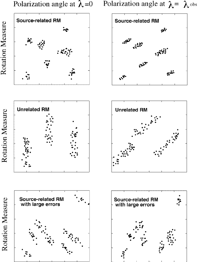
Figure 1: Indication of the expected dependences of rotation measure and polarisation angle for different scenarios.

Figure 1 explores the signatures in the RM-PA plane that would arise from various origins of any observed RM variations. For each case, we present two different plots: 1) RM-PA$(\lambda_{0})$, which is the scatter diagram of RM vs. the zero wavelength polarization position angle as calculated using the RM, and 2) RM-PA$(\lambda_{\rm obs})$, where the polarization angle is simply that observed at some wavelength $\lambda_{\rm obs}$.

The top cartoons first assume that the radio source is composed of a finite number of well-resolved ordered field regions, and that these ordered fields are embedded in a Faraday rotating medium (which might be internal to the source, or on a thin skin). We then make the simplifying and favorable assumption that most observed magnetic field changes in the plane of the sky (giving the PA) will be accompanied by some change along the line of sight (giving the RM). In such a situation, one would then see clusters of points in the RM-PA$(\lambda_{0})$ diagram. Note that in this situation there is not a monotonic relation between PA and RM, i.e., there is no global correlation between the two quantities, only a clumpy distribution.

In the non-idealized case, the clumps will have a finite size for a variety of reasons – errors in the measurement of either quantity, changes in the magnetic field strength along the line of sight that are not well correlated with PA changes, and changes in path length or density of the Faraday rotating medium, which will change the RM, but not PA$(\lambda_{0})$. If any of these confusing factors is sufficiently large, the Faraday rotation may still be physically dominated by the source magnetic structure, but there will be a great deal of scatter in the RM-PA diagram and signatures will be masked. Looking for clumpiness in the PA-RM diagram is thus a one-sided test – if sufficient clumpiness is observed, the RMs originate local to the source; if clumpiness is not observed, this test in isolation does not provide information on the origin of the rotations. Some clumpiness in the RM-PA plane can arise from source structure alone, so this must be carefully evaluated, as discussed below.

Turning now to the correlation of RM with the PA observed at $\lambda_{\rm obs}$, the clumps are stretched and repositioned by the rotation at finite wavelength. At sufficiently large values of $\lambda_{\rm obs}$, the PAs will be scattered over all possible angles. As illustrated here, the clumps in the PA-RM plane can be seen at both $\lambda_{0}$ and $\lambda_{\rm obs}$.

We now examine the signatures of RMs that arise externally and are unrelated to the source. If the RMs vary on small scales (a beam size or less) and are completely unrelated to the source, one simply gets a scatter diagram in the PA-RM plane. This case is not shown. However, the middle set of cartoons illustrates the important situation where there are well-resolved regions of constant polarization angle in the source, as well as well-resolved regions of RM, but which are now completely unrelated to the source. Because of the large scale structures in both parameters, there will be some clumping in the PA-RM plane. To visualize this, suppose there were only three intrinsic polarization angles observed in a source, each covering one-third of the source. Then the diagram would show three clumps in the RM-PA$(\lambda_{0})$ diagram, stretched along the RM axis. In the RM-PA$(\lambda_{\rm obs}$) diagram, these clumps would be rotated and displaced. It is important to separate this misleading clumping, due to unrelated large scale structures in the source and in the external RM distribution, from true correlations. Such an effort is described in the following section.

The final (bottom) set of cartoons in Figure 1 shows the effects of small errors in the RM measurements. Errors within each clump will tend to stretch the clumps in the PA$(\lambda_{0})$ plot to give negative slopes, because the wrong corrections have been applied to the data. Observations at $\lambda_{\rm obs}$ appear similar to the no-error case (top cartoon), but with greater scatter in the RM parameter.

In order to understand the role of measurement errors more fully, we ran a variety of Monte Carlo simulations. We examined the potentially biased situation where coherent large scale errors in PA are actually used to derive the RM, which is then plotted vs. the same PA. In all cases, the distributions in the PA-RM plane looked like either the middle or bottom cartoon in Figure 1. In no case did errors or unrelated RMs cause small-scale clumping, i.e., clumps with an extent significantly smaller than the overall range of RMs. Although this gives us confidence that our results and interpretation are reasonable, it does not guarantee robustness against all possible distributions of PAs and RMs; this is discussed further below.

3 Analysis of PKS 1246$-$410 and Results

We re-examined the polarimetric data on PKS 1246$-$410 of Taylor, Fabian & Allen (2002), kindly provided by G. Taylor, including their RM image, which they derived using maps at 4 frequencies (8.4681, 8.1149, 4.8851 and 4.6351 GHz). We then created polarization angle at $\lambda_{0}$ maps by de-rotating the position angle image at 8.4681 GHz using Taylor et al’s RM map. Taylor, Fabian & Allen (2002) blanked their RM map wherever the residual polarization angle, $\delta{\rm PA}(\lambda_{0})$, at any frequency was greater than 15 degrees. The resolution of their images is 2.1 arcsec by 1.2 arcsec with a beam position angle of 19 degrees.

In this section, we describe in detail the process we used to reach the conclusion that the RM variations in PKS 1246$-$410 had a strong contribution local to the source. First, we describe the construction of simulated maps for comparison with the actual data. Then we use a variety of methods for comparison. Finally, we discuss the limitations to this analysis, and the inferences for the Faraday rotating medium in PKS 1246$-$410.

3.1 Simulated map construction

We created random simulated data to approximate as closely as possible the amplitude and spatial distributions of the RMs measured by Taylor, Fabian & Allen (2002), but which were not linked to source structure (in total or polarised intensity) in any way. These random images were constructed by using the noise-generating feature of the AIPS task IMMOD to create a large noise image, from which three independent simulations could be drawn.

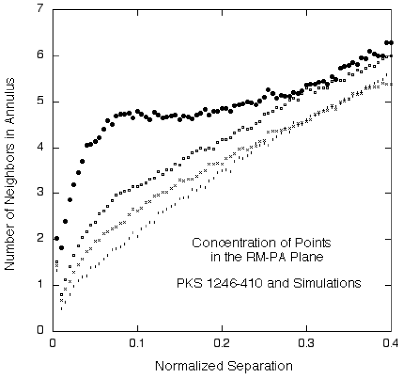
Figure 5: Measurement of the clustering of points in the polarisation angle $-$ rotation measure plane (Figure 4) by counting neighbors in annuli as a function of normalized distance, as described in Section 3.2. The real data are shown as the large solid circles, while the three individual simulations are shown with smaller symbols.

The first step was to reconstruct the amplitude distribution of RMs, which we did by adding together three large, independent gaussian noise images each with a different mean RM and rms RM, to reflect the broad and narrow features in the observed RM amplitude distribution shown in Taylor, Fabian & Allen (2002)’s Figure 5. The simulated RM distribution was then convolved spatially with a circular gaussian of 5 arcsec. This value was picked by trial and error, so that the spatial scales of the simulated RM distributions matched that of the observed RM distribution. A region of the large noise map with the same number of pixels as the actual maps was arbitrarily selected. Then, exactly as for the observed RM map, the simulated random RM map was masked so that only the structure within the silhouette of the source remained.

Three independent regions on the noise map were arbitrarily chosen to create three such simulated RM maps. Finally, both simulated and observed maps were median weight filtered using a box size of 3.2 arcsec (11 pixels), to reduce some of the high spatial frequency scatter. The similarity of the simulated and observed RM distributions can be seen directly in Figures 2 and 3. Figure 2 shows the similarity in amplitude and spatial scale of the observed and simulated RM distributions. Figure 3 uses an autocorrelation function to show quantitatively that the spatial scales are well matched.

3.2 Differences between observed and simulated RM maps

In this section, we will examine the differences between the observed and simulated maps in a variety of ways – visual inspection, a statistical analysis of the clumping in the RM-PA plane (similar to two-point correlation analyses), and finally a one-dimensional correlation/concentration analysis to determine the typical scatter of RMs within clumps in the RM-PA plane.

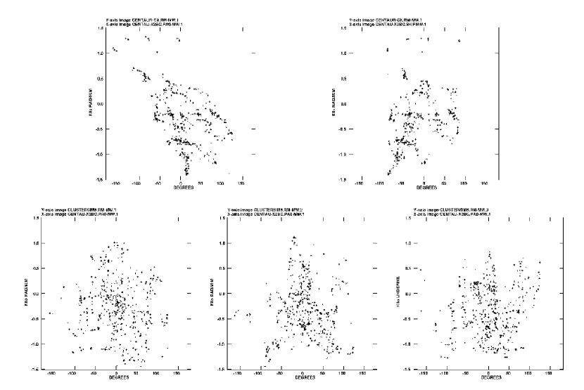
Figure 4: Scatter plot of rotation measures versus polarisation position angles. Top left: actual data as observed at 8.4 GHz; Top right: actual data at 8.4 GHz with angles corrected to zero wavelength, using RMs as plotted; Bottom: simulations, with angles corrected to zero wavelength, as above. See Section 3.1 for description of median-weighted filtering and processing.

Visual inspection of the middle and bottom maps on the left of Figure 2 allows one to pick out corresponding features in the actual PA and RM images. At the same time they indicate how nicely the RM simulations (on the right) mimic the real data without showing any correlations with source structure. This can be seen more clearly in the scatter plots (Figure 4) of RM versus polarisation angle, both corrected for Faraday rotation [PA$(\lambda_{0})$] and uncorrected [PA$(\lambda_{\rm 3.6cm})$]. For the RM-corrected position angles (actual data) we also produced scatter plots versus each of the three independent RM simulations; all plots are shown in Figure 4. For these plots, the data are somewhat oversampled in order to ensure that the sharp observed transitions in PA and RM are included; the actual data and simulations are sampled in exactly the same way.

A visual inspection makes it apparent that the observed data are much more highly clumped than the simulations. In order to examine this clumpiness more quantitatively, we calculated the average number of neighbors around each point in the RM-PA plane, after normalizing each of the PA and RM distributions to zero mean and unit variance. A more rigorous analysis would account for the $180$ degree ambiguity in PA, but would not affect the current results. Figure 5 shows a large excess of neighbors for the real data, compared to the simulations, up to a normalized separation of at least 0.2. The excess at the low end demonstrates that the intrinsic source structure [as indicated by PA$(\lambda_{0})$] is related to the observed RM. A separation of 0.2 corresponds to a difference in PA between two points of 45 deg or 45 rad/m² in RM, or an equivalent combination of the two. These values indicate the scale of both the intrinsic scatter and the errors in RMs within each fairly homogeneous region.

In the idealized limit of the source consisting of a finite number of completely homogeneous components with random field strengths and angles, partially mixed with a thermal plasma, we would expect to see a finite set of tight clumps in the PA$(\lambda_{0})$ versus RM diagram, similar to what is observed. If the RM structure were external to the source, e.g. in the intracluster medium and not connected to the source, then we would expect to see no such clustering in the PA$(\lambda_{0})$-RM plane other than the modest non-uniformities due to the source structure itself, as illustrated in Figure 1. These results indicate that the RMs for PKS 1246$-$410 are related to its own polarization structure.

Note that the clumping is seen for the actual data whether or not RM-corrections have been applied (i.e. for both PA$(\lambda_{\rm 3.6cm})$ and PA$(\lambda_{0})$); therefore the derived RMs are not the cause of the clumping. However, in the RM-corrected position angles we note that there are a variety of clumps which show elongation along a slope of $-0.07$ to $-1.1$ degrees per rad/m² (at $\lambda 3.6$ cm). This is exactly as expected if small RM errors in each major clump contributed to a spread in derived intrinsic position angles, as seen in the bottom cartoon of Figure 1. The RMs are thus significantly more uniform in each region than actually observed. In addition, there is a slight tendency for the overall distribution of clumps to be elongated in the same direction as within individual clumps. This could indicate errors in RM on larger scales, although with only a small number of independent clumps, it is not possible to establish this clearly.

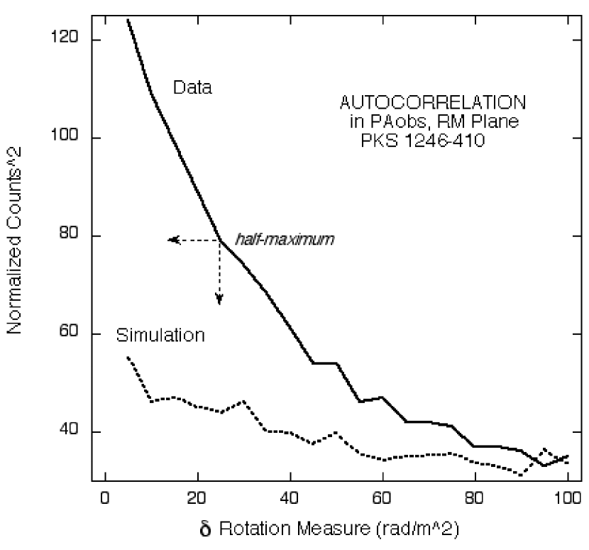
Figure 6: Autocorrelation as a function of shift in RM for the data and first (left) simulation plotted in Figure  4. The dashed lines identify the approximate half-power point of the RM shift above the background autocorrelation level.

We can use the clumping in the PA-RM plane to place a upper limit on the contributions to the RMs in each region from external Faraday media, unrelated to the source. As discussed above, the width of each clump along the RM axis in the PA-RM plane is dominated by small errors, and we can therefore take this width as a conservative limit to the contribution of external RMs. To measure a characteristic width of clumps in the entire plane, we form the one-dimensional autocorrelation of the counts in PA-RM bins as a function of a shift in the RM ($\delta RM$). We first count the number of pixels in bins of 1 $\deg$ in $PA_{\rm obs}$ and $5\,{\rm rad/m}^{2}$ for both PKS 1246$-$410 and the first of our simulations, without any further smoothing, and then sum their one-dimensional autocorrelations. Note that this sum of one-dimensional autocorrelations at each PA is not the same as the autocorrelation of the RM distribution summed over all PAs. The results are shown in Figure 6. The clumping in the PA-RM plane is visible here as an excess at small values of $\delta RM$. At large values of $\delta RM$ the autocorrelation falls to the same value as the simulation, reflecting the overall distribution of RMs. The half-width of the excess at small $\delta RM$s is $\approx 25\,{\rm rad/m}^{2}$, which we therefore take as an upper limit to external contributions.

3.3 Limits to the analysis

Our derived external RM limit applies only over a limited range of scale sizes. Any external RM variations on scales $<3\arcsec$ would be averaged out by the beam size, and so would not be detected in our analysis. At the other extreme, a constant external RM over the entire source would simply move the clumps to a different location in the RM $-$ PA plane, and again, not be detectable. External RMs on scales significantly larger than the coherent field regions (i.e.,$\stackrel{{\scriptstyle>}}{{{\scriptstyle\sim}}}$ 15 arcsec) would thus not be identifiable. The only way to sample such large scale fields is by using the RMs of well-constructed samples of background sources.

Although we have argued that the observed PA-RM clumping is easily distinguishable from the effects of random external RM distributions, this is based on a reasonable, but simple, set of assumptions. In particular, we assume that we can model uncorrelated external cluster RM contributions by random gaussian noise matched in both its RM amplitude distribution and in its distribution of RM patch scale sizes. We have shown by Monte Carlo simulations, again based on random gaussian fluctuations, that measurement errors do not create the observed clumping. We do not, however, prove that our analysis is robust against all possible RM and PA distributions, especially involving higher order correlations. For example, we have not modeled the possible effects of large scale gradients in the RMs, or a tendency for extreme RMs to be closer together or further apart than expected at random. Such an open-ended exploration is beyond the scope of this paper. It is also not clear what the utility of such an exploration would be; if one finally found a distribution that reproduced the observed RM-PA clumping, it would simply show that an external RM source is possible, not necessarily likely. However, it would be interesting to explore physically motivated models of cluster magnetic field structures, and determine their manifestations in the PA-RM plane, and whether these could be distinguished from local source effects.

3.4 Inferences regarding PKS 1246$-$410’s Faraday rotating medium

Converting the RM limit of $\approx 25\,{\rm rad/m}^{2}$ into a limit on the magnetic field in the cluster medium around PKS 1246$-$410 is a model-dependent process as discussed by Newman et al (2002). One must make assumptions about the dependence of both the electron density and the magnetic field strength as a function of the distance from the cluster center, and the coherence length of the magnetic field. As shown by Newman et al (2002), reliable measurements or limits to the field depend on conducting Monte-Carlo simulations of the expected RM distribution under a given set of assumptions about the cluster. Such a calculation is beyond the scope of this work, and we simply use our upper limit in the identical way to Taylor, Fabian & Allen (2002) for comparison with other numbers in the literature. Taylor, Fabian & Allen (2002) use the overall RM dispersion of $660\,{\rm rad/m}^{2}$ and X-ray measurements of the Centaurus cluster from Allen et al (2001b) and Sanders & Fabian (2002) to estimate a strength of $11\mu{\rm G}$ for magnetic fields which vary on scales of 1 kpc ($3.6\arcsec$). Using our limit of $25\,{\rm rad/m}^{2}$ for external contributions, we conclude that the strength of magnetic field variations in the intracluster medium on this scale is $<0.4\mu{\rm G}$. We note again that such a derivation is highly model dependent.

Further information about the Faraday rotating medium comes from the observed depolarization between 8.1 GHz and 4.6 GHz. Figure 7 shows the fractional polarizations between these two bands plotted against each other. Two things are worth noting – the very high fractional polarization present in some parts of Taylor et al’s image and the strong mean depolarization ($\%Pol_{4.6GHz}/\%Pol_{8.1GHz}\approx 0.3$).

There are two general ways in which sources can become depolarized, due to internal or “external” variations in RM (Burn, 1966). We start with the less popular alternative of internal depolarization (e.g., Jagers (1987)). In this case, a thermal plasma is mixed with the relativistic plasma, and along any line of sight the rotation from regions near the back of the source will be rotated by different angles from those near the front, with more destructive interference at longer wavelengths. We can examine the plausiblity of this idea by supposing that the X-ray emitting gas, (Allen et al, 2001b; Sanders & Fabian, 2002) with central density $n_{0}\approx 0.1{\rm cm}^{-3}$ has penetrated throughout the source. The maximum RM (and depolarization) will occur in the limiting, although unrealistic, case of a uniform field from front to back, without field reversals. Using a minimum energy field strength of $\approx 10\mu{\rm G}$ and a line of sight path length of $\approx 3$ kpc would yield a total RM of 1400 ${\rm rad/m}^{2}$ through the source, comparable to the largest values observed. At 4.6 GHz, this corresponds to a $\lambda^{2}$-equivalent rotation of $\approx 340\deg$, which would correspond to a front-to-back depolarization by a factor $\approx 40$ in the simplest slab geometry (e.g., Burn (1966); Cioffi & Jones (1980)). On the basis of these numbers alone, one could try to construct more realistic geometries for an internal depolarization model. However, internal depolarization models result in very limited rotations in observed polarization angle (e.g., $45-90\deg$, depending on geometry, Cioffi & Jones (1980)), not the $\approx 360\deg$ observed for PKS 1246$-$410.

In the case that the depolarization is caused “externally”, this could either be in a thin skin along the boundaries of the source, in the medium directly influenced by the source, or in the completely unrelated foreground. In all cases, where the rotation measure changes rapidly from one beam to the next, the depolarization will be strongest, as is observed. A typical change of 600 rad/m² between RM clumps results in an angle change of $\approx 45(135)\deg$ at 8.1 (4.8) GHz, resulting in much more destructive interference at the lower frequency. Unfortunately, there is no clear signature in the depolarization to isolate the location of the “external” medium, and thus whether it is the magnetic field at the source boundaries, or an intracluster field, that is responsible for the depolarization.

4 Correlated RM-PA variations in other sources

PKS 1246$-$410 presented a fortuitously powerful laboratory in which to search for source-related Faraday effects, because of its very high fractional polarization. In such a case, there are probably few if any field reversals along the line of sight. Thus, wherever the Faraday rotation is taking place in the source, be it a thin skin, or an extended distribution of thermal plasma, the magnetic field along the line of sight should be simply related to the observed polarization angle on the sky. In most radio sources, with lower fractional polarizations, the situation is much less clear.

In general, we expect to see only an occasional correspondence between the RM and local magnetic field direction, even if the rotation is completely local to the source. In addition to probing different components of the magnetic field, only the RM is sensitive to fluctuations in thermal density, and the field near the surface will typically differ from the line of sight averaged field in the plane of the sky. Therefore, even isolated regions of correspondence can provide evidence for RM contributions local to the source.

We have examined in less detail the correspondence between observed RM and the polarization position angle in three 3C sources, and find some closely related features in the two parameters, as described below. This has important consequences for the use of RM variations in cluster radio galaxies to derive values for the (unrelated) magnetic field variations in the intracluster medium. Such a derivation can only be done after the RM contributions local to the source are removed, a task that would be extremely difficult to accomplish. In the presence of source-related RMs, it is still possible to set upper limits to cluster fields, but not to determine their magnitude.

4.1 3C 75 and 3C 465

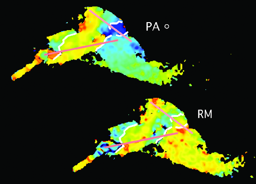
Figure 8: Maps of the derived magnetic field direction (left, upper) and RM (right, lower) of the northern tail of 3C 465 from Eilek & Owen (2002); the E-W extent of the source is $\approx 120\arcsec$; North is directly up. Position angles vary from $-90$(blue) to $90$ (red) degrees. Rotation measures vary from $\approx-200$ (blue) to $100$ (red) rad/m². White lines indicate some of the regions where there are corresponding transitions in both quantities. The off-white lines show the location of one-dimensional slices plotted in Figure  9. The beam size is indicated by the white circle.

Figure 8 shows the derived magnetic field direction (left, upper) and RM (right, lower) maps of the northwestern tail of 3C 465 from Eilek & Owen (2002) and kindly provided by them. The northwestern tail provided a wide range of magnetic field directions, spanning at least 120$\deg$ which we could examine for correlations with the local RMs. By contrast, the southern tail provided only about 30$\deg$ of magnetic field angle variation, insufficient to allow a correlation search. However, Eilek & Owen (2002) do note that even in the southern tail, the extreme RMs ($\pm 200{\rm rad/m}^{2}$) are found to be associated with the hot spot.

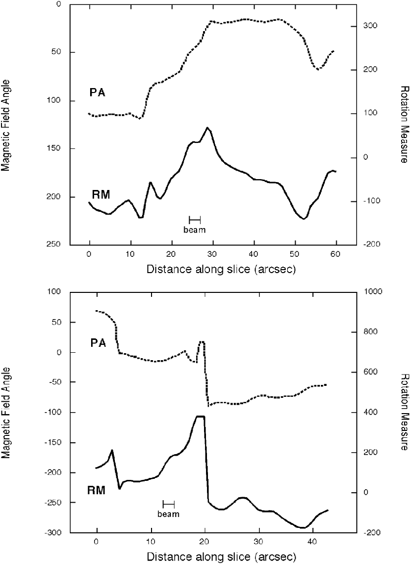
Figure 9: One-dimensional slices in RM and magnetic field direction along the lines shown in Figure 8

In the northwestern tail we find some places where the magnetic field direction and the RM both undergo sharp changes, as indicated in Figure 8. These transitions can be more clearly seen in the one-dimensional slices (Figure 9) at the locations indicated in Figure 8. Note that the beam size is much smaller than the regions of coherent magnetic field direction. The indicated transitions in RM and magnetic field direction occur against a much smoother background, and are not the result of random small-scale variations. These figures and slices demonstrate that a relationship exists between the magnetic field direction and the RM at least in some locations in 3C465, and therefore a significant part of the observed Faraday rotating medium is local to the source, as in PKS 1246$-$410.

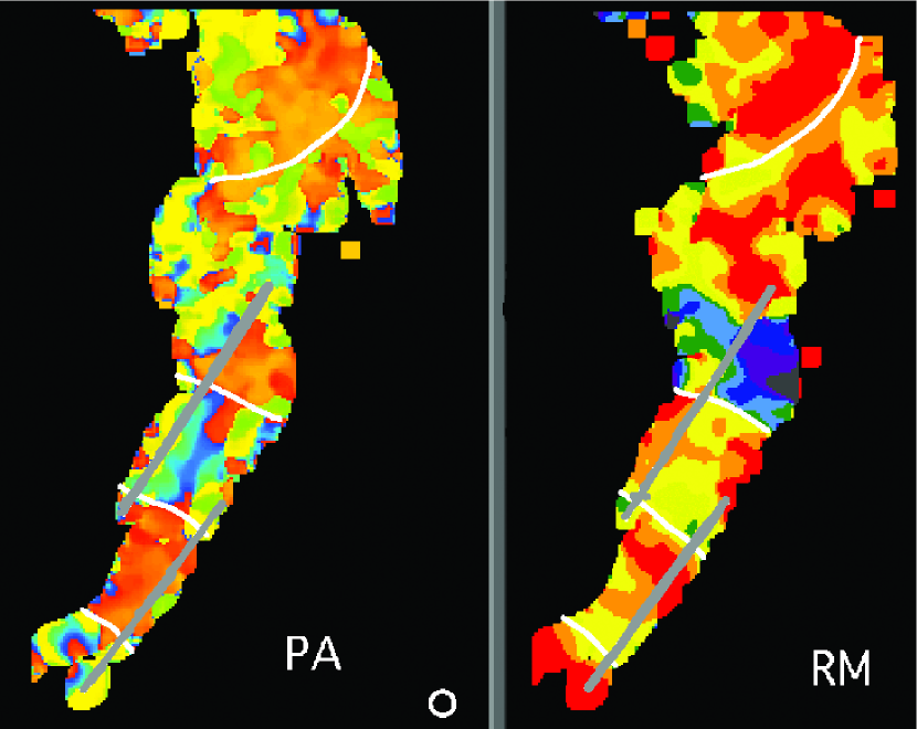
Figure 10: Same as Figure  9, but for the northern tail(s) of 3C75. The N-S extent of the source is $\approx 110\arcsec$; North is directly up. Position angles vary from $-90$(blue) to $90$ (red) degrees. Rotation measures vary from $\approx-100$ (blue) to $100$ (red) rad/m².

3C 75, again from Eilek & Owen (2002), provides another example of correlated changes. Only the northern tail(s) are shown here, because they contained sharper transitions in magnetic field direction and therefore clearer examples of correlated changes. We note again that given the various factors, as discussed in Section 2, that can independently influence the RM and magnetic field angles, we expect only isolated correlations. We first smoothed the data with a median weight filter of five pixels (less than one beam) which reduces some of the smallest scale mottling. A complication that arises in this analysis comes from the 180 degree ambiguities in magnetic field direction. A smooth transition, e.g., from 170 degrees to 190 degrees will appear as a large jump if the latter is recorded as $-10$ degrees. In our analysis of 3C 75, we found a number of apparent jumps (also see Eilek & Owen (2002)) and arbitrarily added 180 degrees to smooth the magnetic field angles as much as possible. The resulting PA and RM distributions for the northern half of 3C 75 are shown in Figure 10, with the corresponding slices in Figure 11. There still remains an overall 180  degree ambiguity in the regions where the magnetic field variations were smoothed. Therefore, in the slices, we show both possibilities, and note that the corresponding transitions in magnetic field direction and RM appear in either case.

4.2 Cygnus A

Bicknell et al (1990a, b) find that at least some of the RM features in Cygnus A are associated with features in the total intensity image which they call surface waves. This is an unusual case, because total intensity structures often show little or no correspondence to RMs. Perley & Carilli (1995) also find one specific RM - total intensity relationship in the distinct semi-circular region surrounding hotspot “B”, which Carilli, Perley & Dreher (1988) interpreted as due to a bow shock caused by the hotspot; Perley & Carilli (1995) do not find other RM - total intensity correspondences in the jet and hotspot features.

In the case of Cygnus A, Bicknell et al (1990a, b) propose that the intensity related RM structures arise from non-linear Kelvin-Helmholtz waves in a mixed magnetic field and thermal plasma. These give rise to large rotation measure variations on the scale-size of the waves. Such a model would be consistent with the fact that the overall pattern in RM is the same in each lobe. Moreover, being a surface effect, this would give rise to a dependence of RM on $\lambda^{2}$. Dreher et al (1987) observed such a $\lambda^{2}$ dependence of polarization angle, and eliminated internal Faraday rotation in Cygnus A; they also eliminate a Galactic origin. Although Dreher et al.’s abstract states that they propose the origin of the rotation measure is in the intra-cluster gas, their conclusions describe how the Faraday screen could equally well be the intra-cluster gas or a sheath around the lobes, a possibility we consider further, and favour, in Section 5.

5 Implications of a source-related Faraday medium

We have shown that for PKS 1246$-$410 the RM variations across the source are likely to be dominated by a Faraday medium associated with the source itself, with little or no cluster field contribution. Indications of source-related RM variations were also shown for 3C75, 3C465 and Cygnus A. These results have important implications both for studies of intracluster magnetic fields as well as for the physics of radio galaxies. In this section, we look briefly at issues such as the role of mass entrainment in cluster sources, the presence of warm, dense optically emitting gas, the trend for higher RMs toward cluster centers, the radio luminosity dependence of depolarization, the side-to-side depolarization asymmetries seen in some samples of radio galaxies and quasars, and statistical RM probes of cluster fields.

5.1 Entrainment

Entrainment is likely to be a common feature of FR I jets. For example, Bicknell (1994) has used the conservation laws to demonstrate the relationship between entrainment and deceleration. In a similar manner, Laing & Bridle (2002) find that mass-loading or entrainment of ambient matter is required to reproduce the observed deceleration in the jets of FR I radio galaxy 3C 31. Once thermal matter is entrained within the magnetic field of the synchrotron emitting plasma it must at least be considered as contributing to observed Faraday Rotation. Without considering entrainment, which could appear as correlations in the RM-PA plane as discussed here, cluster magnetic field strength estimates can get very high, for example, $\approx 10\mu{\rm G}$ in Abell 119 (Feretti et al, 1999) or $\approx 35\mu{\rm G}$ in Hydra A (Taylor et al, 1993). The current work shows that such derivations are not justified.

In addition to direct mixing of the thermal and relativistic plasmas, radio sources in clusters can have a dramatic influence on the surrounding medium. Holes in the hot X-ray emitting plasma are seen, for example, around radio sources in the Perseus (Böhringer et al, 1993; Fabian et al, 2002) and Hydra (McNamara et al, 2000) clusters. Bouyant bubbles from Centaurus A also appear to have influenced the external medium (Saxton, Sutherland & Bicknell, 2001). Therefore, in addition to Faraday rotation from material which is directly mixed with the radio plasma, there could also be contributions from the ICM which are correlated with the radio source properties. In such a situation, the magnetic field strengths derived from the RMs would apply to the ICM influenced by the source, but could not be used to measure cluster-wide fields.

5.2 RM trends toward cluster centers

There appears to be a trend that radio sources closer to the cluster center show higher RM variations than those further out (Feretti et al, 1999; Taylor et al, 2001; Govoni et al, 2001; Dolag et al, 2001). Although this has been interpreted as demonstrating the existence of cluster-wide fields, two factors indicate that a Faraday medium local to the source, as suggested here, is also consistent with the data. First, cluster sources are almost exclusively FR Is, showing distorted morphologies that are usually understood as due to mass loading and entrainment of the surrounding medium (as discussed in Section 5.1). Second, the environments are indeed denser towards the centers of clusters, so even if the penetration of source fields into a thin skin of thermal material were the same for all sources, we would see larger Faraday effects in the vicinity of the cluster centre. Similarly, the high densities in cooling flow clusters would lead to high rotation measures for any embedded sources, (e.g., Taylor, Fabian & Allen (2002)), independent of any cluster-wide fields. It is critical to remove the dependence of source-related RMs on their local surrounding density before making any claim for stronger fields towards the centers of clusters.

5.3 Optically emitting gas as a Faraday medium

Several theoretical arguments have been made to show that the RMs of embedded cluster sources cannot plausibly arise local to the source. One argument is that a fully mixed thermal plasma would greatly depolarize the sources (Dreher et al, 1987). It has been suggested that even a thin skin of thermal material can be problematic as the origin for RMs (Taylor et al, 1993; Ge & Owen, 1993; Eilek & Owen, 2002) , based either on geometric arguments or the very high inferred strengths for magnetic fields near the source boundaries. However, most of these arguments are based on the restrictive and unjustified assumption that the only thermal material available is the diffuse hot X-ray emitting plasma. Even in this restrictive case, Table 1 in Eilek & Owen (2002) shows that a partially mixed hot plasma could produce the observed RMs in 3C75; this is not reflected in their discussions or conclusion.

Wherever one could document the implausibility of hot gas as the Faraday medium, it is still necessary to consider the effects of gas at $10^{4}-10^{5}$K. There is an extensive literature documenting the presence of warm, dense emission-line material in the centers of rich X-ray clusters (Heckman, 1981; Cowie et al, 1983; Hu, Cowie, & Wang, 1985; Koekemoer et al, 1999). These emission-line systems are often found to be interacting with radio galaxies on scales of 10s to over 100 kpc (Heckman, van Breugel & Miley, 1984; Baum & Heckman, 1989; McCarthy et al, 1990), and in the cases of A  2597 and Coma  A, for example, form a clear boundary layer around the radio lobes (Koekemoer et al, 1999; Tadhunter et al, 2000). Such material causes regions of strong depolarization (Heckman, van Breugel & Miley, 1984; Pedelty et al, 1989a; Chambers, Miley & van Bruegel, 1990) and must therefore also contribute to the RM wherever the medium is slightly more Faraday transparent.

In situations where this gas is slightly less dense, or not yet sufficiently cooled, it will not be prominent in emission lines, but can still be a very effective Faraday medium with a modest amount of field penetration into the radio source. In 3C75, for example, Owen, O’Dea & Keel (1990) use long-slit spectroscopy to set limits on the density and temperature of cooler gas in pressure equilibrium with the surrounding hot cluster medium. For a 2.5 kpc cloud, they find that the temperature must be above $2.5\times 10^{5}$K, yielding a density at pressure matching of $\approx 0.2{\rm cm}^{-3}$. If 3C75’s magnetic field were also in pressure equilibrium with this gas (6 $\mu{\rm G}$ , Eilek & Owen (2002)), then it would produce an RM of $\approx 2500{\rm rad/m}^{2}$, 25 times higher than the RMs observed in this source. This shows that sufficient warm material to produce the observed RMs is still allowed by the observations; it does not demonstrate that this material actually exists. We can also ask whether sufficient gas to cause the RMs could be at the more plausible temperature of $10^{4}$ K. Using the same size cloud as above, and relaxing the pressure balance criterion, we need material only $0.04$ times as dense as above to produce the observed RMs. The emissivity would then go up by $\approx 25$ because of the lower temperatures (see Fig. 7 in Owen, O’Dea & Keel (1990)), and down by $\approx 0.002$ because of the lower density, and would thus not have been detected. Owen, O’Dea & Keel (1990) also report observations of 3C465. However, their slit did not cover any of the northern tail discussed in this paper.

Given the common appearance of emission line systems, and even the currently available limits, we consider it quite plausible that the cluster sources showing large RM variations are interacting with a dense, warm medium. Searches for additional emission line systems, (e.g., Tadhunter et al (2000), Owen, O’Dea & Keel (1990)) and kinematics of this material (e.g. Hu, Cowie, & Wang (1985)) could be of great benefit both in understanding the physics of the radio sources and their energy input to the intracluster medium. Further exploration of sources showing Faraday effects intrinsic or local to the source (Pedelty et al, 1989b; Liu & Pooley, 1991; Best et al, 1998; Ishwara-Chandra et al, 1999) would also be useful, as well as demonstrating why they cannot be used to derive unrelated cluster field strengths.

5.4 RM trends in samples of radio galaxies

Garrington & Conway (1991), in their Figure 2, show that the Faraday dispersion for a sample of classical double FR IIs is an increasing function of $z$ (and thus luminosity in a flux-limited sample). Pentericci et al (2000) show how the fraction of high RM sources strongly increases with redshift. Are these telling us about the large-scale environment of these sources (Carilli et al, 1997; Pentericci et al, 2000), or about the properties of the sources themselves? Before a claim for environmental effects is possible, corrections for luminosity effects would have to be determined and made. In all current models for radio-galaxy evolution, higher luminosity sources have higher magnetic field strengths; in the thin-skin Faraday rotation proposed here, this would automatically lead to higher depolarizations and RMs in high-luminosity sources as observed, even if the external densities were the same for all sources. It is therefore premature to interpret the luminosity/Faraday relations as due to a denser environment at large redshifts (luminosities), although that might be demonstrated to be the case in the future. A further claim that such relations imply a large scale magnetized cluster gas, separate from the sources themselves (Carilli et al, 1997) is an untested assumption until the individual radio sources can be examined for source-related Faraday contributions, as done in this paper.

Similarly, the lower level of depolarization seen in the (presumably nearer, Doppler-boosted) jetted side compared to the non-jetted side of some samples of radio sources (originally suggested by Laing (1988) and Garrington et al (1988)) has been cited as evidence for an extended, magnetized halo (e.g., Garrington & Conway (1991)). However, we note that such an asymmetry merely demonstrates (and requires) the existence of a medium on the same scale as a particular radio source that shows this effect, and, in any case, requires magnetic fields of only $\approx 1\mu{\rm G}$ in a hot medium for sources with $1\leq z\leq 2$.

5.5 Statistical searches for cluster fields

In addition to attempts to measure Faraday rotation through the intracluster medium using individual sources, as discussed above, there have been a number of efforts to look for an excess RM using background sources in the directions of clusters of galaxies compared to samples away from clusters. There are several sets of work reporting incompatible results (e.g., Clarke, Kronberg & Böhringer (2001); Kim, Tribble & Kronberg (1991); Hennessy, Owen & Eilek (1989)). In a separate paper, we present a thorough analysis of these studies. At present, we note that the current paper’s results on individual radio galaxies in clusters show that some or all of their RM variations are local to the source, and can thus not be used to measure cluster fields. Unfortunately, the most recent and extensive work on sources seen “through” clusters (Clarke, Kronberg & Böhringer, 2001) has a cluster sample that is dominated by radio galaxies actually embedded in the clusters under study, i.e., not background sources. When all problematic sources are removed from the samples of Hennessy, Owen & Eilek (1989) and Clarke, Kronberg & Böhringer (2001), there is little, if any, evidence remaining for cluster fields at the claimed $>1\mu{\rm G}(>0.1{\rm nT})$ levels (Rudnick & Blundell, 2003). Newman et al (2002) have provided an additional critique of the statistics presented by these studies, demonstrating serious problems with how RM limits or values are translated into field strength estimates.

6 Conclusions

Given the existence of a Faraday medium connected to individual radio galaxies, we conclude that the claims for strong intracluster magnetic fields, 1 $-$ 40 $\mu{\rm G}$ ( 0.1$-$4 nT), based on studies of individual radio galaxies are not warranted by careful consideration of the current data. The current best estimates for cluster field strengths are in the $<1\mu{\rm G}$ ($<0.1$ nT) range, from cluster synchrotron halos or inverse Compton measurements (see refs in Carilli & Taylor, 2002) and from theoretical arguments from the early universe (Barrow et al, 1997). There is, in addition, a great opportunity to learn about the physics of radio galaxies from a more detailed study of their Faraday rotating skins.

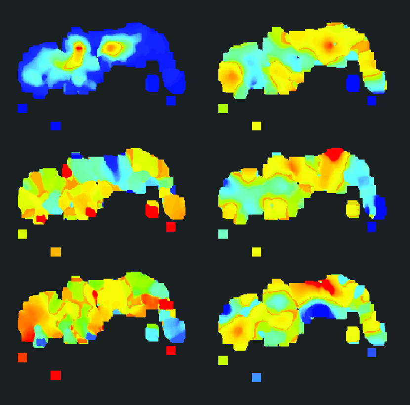
Figure 2: Distribution of polarisation structures in PKS 1246$-$410. The source is $\approx 30\arcsec$ long; North is directly up. Left column $--$ actual data from Taylor et al. (2001) top: polarized intensity, at 8 GHz, peak flux density 4 mJy/beam (red); middle: rotation measure, $\approx-1300$(blue) to $1300$(red) rad/m²; bottom: RM-corrected position angle ($-90$(blue) to $+90$(red) degrees. Right column $--$ simulations of rotation measure, with same color scale as actual rotation measure at left middle. See Section 3.1 for processing information.

Figure 3: Autocorrelation functions of the real and simulated RM distributions showing that they have the same spatial scale structures. The simulated autocorrelation shown is the average of the three individual simulation correlations.

Figure 7: Fractional polarization at 4.6 GHz vs. that at 8.1 GHz. Lines of no depolarization (D=1) and depolarization by a factor of 10 (D=0.1) are shown. Note both the very high fractional polarizations present and the strong average depolarization. There are approximately 2 points plotted per independent beam area. Pixels that were blanked for the RM image, as described in Section 3.1, are not included here.

.

Figure 11: One-dimensional slices in RM and magnetic field direction along the lines shown in Figure 10. Two versions of the magnetic field slices are shown, with different choices for resolving 180 degree ambiguities.

References

- Allen et al (2001a) Allen, S. W., Taylor, G.B., Nulsen, P. E. J., Johnstone, R. M., David, L. P., Ettori, S., Fabian, A.C., Forman, W., Jones, C., & McNamara, B., 2001a, MNRAS, 324, 842
- Allen et al (2001b) Allen, S. W., Fabian, A.C., Johnstone, R. M., Arnaud, K.A., Nulsen, P. E. J., 2001b, MNRAS, 322, 589
- Bahcall & Soneira (1984) Bahcall, N. A. & Soneira, R. M., 1984, ApJ, 277, 27
- Barrow et al (1997) Barrow, J.D., Ferreira, P.G. & Silk, J., 1997, Phys. Rev. Lett., 78, 3610
- Baum & Heckman (1989) Baum, S. A., & Heckman, T., 1989, ApJ, 336, 681
- Best et al (1998) Best, P. N., Carilli, C. L., Garrington, S. T., Longain, M. S., & Röttgering, H. J. A. 1998, MNRAS, 29, 357
- Bicknell et al (1990a) Bicknell, G.V., Cameron, R.A. & Gingold, R.A., 1990, in ‘Galactic and Intergalactic Magnetic Fields’, Eds R. Beck, P. Kronberg, R. Wielebinski, Kluwer, p477
- Bicknell et al (1990b) Bicknell, G.V., Cameron, R.A. & Gingold, R.A., 1990, ApJ, 357, 373
- Bicknell (1994) Bicknell, G. V. 1994, ApJ442, 542
- Böhringer et al (1993) Böhringer, H., Voges, W., Fabian, A. C., Edge, A. C. & Neumann, D. M., 1993, MNRAS, 264, l25
- Burn (1966) Burn, B.J., 1966, MNRAS, 133, 67
- Carilli, Perley & Dreher (1988) Carilli, C. L., Perley, R. A., & Dreher, J. W., 1988, ApJ, 334, l73
- Carilli et al (1997) Carilli, C. L., Roettgering, H. J. A., van Ojik, R., Miley, G. K., van Breugel, W. J. M., 1997, ApJS, 109, 1
- Carilli & Taylor (2002) Carilli, C.L. & Taylor, G.B., 2002, ARA&A, 40, 319
- Chambers, Miley & van Bruegel (1990) Chambers, K. C., Miley, G. K. & van Bruegel, W. J. M, 1990, ApJ, 363 21
- Clarke (1999) Clarke, T.E., 1999, PhD thesis, University of Toronto
- Clarke, Kronberg & Böhringer (2001) Clarke, T.E., Kronberg, P.P. & Böhringer, H., 2001, ApJ, 547, L111
- Cioffi & Jones (1980) Cioffi, D.F. & Jones T.W., 1980, AJ, 85, 368
- Cowie et al (1983) Cowie, L. L., Hu, E., Jenkins, E.G. & York, D. B., 1983, ApJ, 272, 29
- Dolag et al (2001) Dolag, K., Schindler, S., Govoni, F., & Feretti, L., 2001, A&A, 378, 777
- Dreher et al (1987) Dreher, J.W., Carilli, C.A. & Perley, R.A., 1990, ApJ, 316, 611
- Eilek & Owen (2002) Eilek, J.E. & Owen, F.N., 2002, ApJ, 567, 202
- Fabian et al (2002) Fabian, A. C., Celotti, A., Blundell, K. M., Kassim, N. E., Perley, R. A., 2002, MNRAS331, 369
- Feretti et al (1999) Feretti, L., Dallacasa, D., Govoni, F., Giovannini, G., Taylor, G.B. & Klein, U., 1999, A&A, 344, 472
- Garrington et al (1988) Garrington, S. T., Leahy, J. P., Conway, R. G., & Laing, R. A., 1988, Nature, 331, 147.