Evolution of massive stars with rotation and mass loss

Abstract

Rotation appears as a dominant effect in massive star evolution. It largely affects all the model outputs: inner structure, tracks, lifetimes, isochrones, surface compositions, blue to red supergiant ratios, etc. At lower metallicities, the effects of rotational mixing are larger; also, more stars may reach critical velocity, even if the initial distribution of rotational velocities is the same.

Geneva Observatory, CH–1290 Sauverny, Switzerland

1. Introduction

In this review, we shall concentrate mostly on the rotational properties of massive stars. Rotation has an importance which for massive stars in the Galaxy is comparable to that of mass loss by stellar winds. For massive stars at lower metallicities, it is likely that rotation plays an even more important role.

2. Structure, mixing and mass loss of rotating stars

2.1. Structure

The equations of stellar structure for a rotating star were written by Kippenhahn & Thomas (1970). These equations apply to a star in solid body or cylindrical rotation. For stars in differential rotation, the use of the above equations is incorrect. Here, we consider the case of shellular rotation with $\Omega=\Omega(r)$ (Zahn 1992). In this case, the structure equations need to be modified (Meynet & Maeder 1997). Structural effects due to the centrifugal force are in general small in the interior. However, the distorsion of stellar surface may be large enough to produce significant shifts in the HR diagram (Maeder & Peytremann 1970).

2.2. Internal transport

For the transport of chemical elements, we consider the effects of shear mixing, of meridional circulation and their interactions with the horizontal turbulence. For shellular rotation, the equation of transport of angular momentum in the vertical direction is in lagrangian coordinates (Zahn 1992),

$$\rho\frac{d}{dt}\left(r^{2}\Omega\right)_{M_{r}}=\frac{1}{5r^{2}}\frac{\partial}{\partial r}\left(\rho r^{4}\Omega\;U(r)\right)+\frac{1}{r^{2}}\frac{\partial}{\partial r}\left(\rho D_{\mathrm{shear}}\;r^{4}\frac{\partial\Omega}{\partial r}\right).$$ (1)

$\Omega(r)$ is the mean angular velocity at level $r$. $U(r)$ is the radial term of the vertical component of the velocity of the meridional circulation. $D_{\mathrm{shear}}$ is the coefficient of shear diffusion. From the two terms in the second member, we see that advection and diffusion are not the same. Thus, the transport of angular momentum by circulation cannot be treated as a diffusion. For the changes of the chemical elements due to transport, we may use a diffusion equation with a diffusion coefficient which is the sum of $D_{\mathrm{shear}}$, as given below, and of $D_{\rm eff}=\frac{\mid rU(r)\mid^{2}}{30D_{h}}$. $D_{\rm eff}$ expresses the resulting effect of meridional circulation and of a large horizontal turbulence (Chaboyer & Zahn 1992). This expression of $D_{\rm eff}$ tells us that the vertical advection of chemical elements is inhibited by the strong horizontal turbulence characterized by $D_{\rm{h}}$. The usual estimate of $D_{\mathrm{h}}=\frac{1}{c_{\mathrm{h}}}r\;|2V(r)-\alpha U(r)|$ was given by Zahn (1992). A recent study suggests that this coefficient is at least an order of magnitude larger (Maeder 2002),

$$D_{\mathrm{h}}=A\;r\;\left(r\overline{\Omega}(r)\;V\;\left[2V-\alpha U\right]\right)^{\frac{1}{3}}\quad\mathrm{with}\quad A=\left(\frac{3}{400n\pi}\right)^{\frac{1}{3}}\;.$$ (2)

For n=1, 3 or 5 $A\approx 0.134,0.0927,0.0782$ respectively. For the coefficient $D_{\mathrm{shear}}$, we use the results by Maeder (1997), Talon & Zahn (1997) and Maeder & Meynet (2001). $D_{\mathrm{shear}}$ is also modified by the horizontal turbulence $D_{\mathrm{h}}$, in the sense that a larger $D_{\mathrm{h}}$ leads to a decrease of the mixing of elements,

$$D_{\mathrm{shear}}=\frac{(K+D_{\mathrm{h}})}{\left[\frac{\varphi}{\delta}\nabla_{\mu}(1+\frac{K}{D_{\mathrm{h}}})+(\nabla_{\mathrm{ad}}-\nabla_{\mathrm{rad}})\right]}\;\times\frac{H_{\mathrm{p}}}{g\delta}\;\left[\alpha\left(b\;\Omega{d\ln\Omega\over d\ln r}\right)^{2}-4(\nabla^{\prime}-\nabla)\right]\;,$$ (3)

with b=0.8836. The radial component $U(r)$ in Eqs. (1) and (2) was given by Maeder & Zahn (1998),

$$U(r) = \frac{P}{\overline{\rho}\overline{g}C_{\!P}\overline{T}\,(\nabla_{\rm ad}-\nabla+(\varphi/\delta)\nabla_{\mu})}\times{\frac{L}{M_{\star}}\left[E_{\Omega}+E_{\mu}\right]+\!\frac{C_{P}}{\delta}\frac{\partial\Theta}{\partial t}\!},$$ (4)

where $M_{\star}=M\left(1-\frac{\Omega^{2}}{2\pi G\rho_{\rm{m}}}\right)$ is the reduced mass, with the notations given in the quoted paper. The driving term in the square brackets in the second member is $E_{\Omega}$. It behaves mainly like,

$$E_{\Omega}\simeq\frac{8}{3}\left[1-\frac{{\Omega^{2}}}{2\pi G\overline{\rho}}\right]\left(\frac{\Omega^{2}r^{3}}{GM}\right).$$ (5)

The term $\overline{\rho}$ means the average on the considered equipotential. The term with the minus sign in the square bracket is the Gratton–Öpik term, which becomes important in the outer layers due to the decrease of the local density. It can produce negative values of $U(r)$. A negative $U(r)$ means a circulation going down along the polar axis and up in the equatorial plane. This makes an outwards transport of angular momentum, while a positive $U(r)$ gives an inward transport of angular momentum. Before, the term $\nabla_{\mu}$ was never properly included. The justification for this term is not so straightforward (Maeder & Zahn 1998).

Figure 1.: Left: The second critical velocity $v_{\mathrm{crit,2}}$ expressed as a fraction of $v_{\mathrm{crit,1}}$ plotted as a function of the Eddington factor $\Gamma_{\mathrm{max}}$, which is the largest value of the Eddington factor over the stellar surface. Right: Evolution of the surface velocities for a 60 M_⊙ star with 3 different initial metallicities.

2.3. Critical velocity and mass loss in a rotating star

For a rotating star, one must consider the flux $F(\vartheta)$ at a given colatitude $\vartheta$ as given by von Zeipel’s theorem. This theorem has been studied for a star with shellular rotation by Maeder (1999), who finds $F(\vartheta)=-\frac{L(P)}{4\pi GM_{\star}}g_{\rm{eff}}[1+\zeta(\vartheta)]$, which shows a small extra–term $\zeta(\vartheta)$ depending on $\Omega,T,\nabla T,\rho$ and opacities. In a rotating star, the Eddington factor becomes a local quantity $\Gamma_{\Omega}(\vartheta)$. We define it as the ratio of the local flux $F(\vartheta)$ given by the von Zeipel theorem to the maximum possible local flux, which is $F_{\mathrm{lim}}(\vartheta)=-\frac{c}{\kappa(\vartheta)}g_{\mathrm{eff}}(\vartheta)$. Thus, one has

$$\Gamma_{\Omega}(\vartheta)=\frac{F(\vartheta)}{F_{\mathrm{lim}}(\vartheta)}=\frac{\kappa(\vartheta)\;L(P)[1+\zeta(\vartheta)]}{4\pi cGM\left(1-\frac{\Omega^{2}}{2\pi G\rho_{\rm{m}}}\right)}\;,$$ (6)

where the opacity $\kappa(\vartheta)$ depends on the colatitude $\vartheta$, since $T_{\mathrm{eff}}$ also depends $\vartheta$. The Eddington factor depends on the angular velocity $\Omega$ on the isobaric surface. This shows that the maximum luminosity of a rotating star is decreased by rotation. It is to be stressed that if the limit $\Gamma_{\Omega}(\vartheta)=1$ happens to be met in general at the equator, it is not because $g_{\mathrm{eff}}$ is the lowest there, but because the opacity is the highest! Indeed, the dependences of $F(\vartheta)$ and of $F_{\mathrm{lim}}(\vartheta)$ with respect to $g_{\mathrm{eff}}$ have cancelled each other in $\Gamma_{\Omega}(\vartheta)$.

Often, the critical velocity in a rotating star is written as $v^{2}_{\rm{crit}}=\frac{GM}{R}(1-\Gamma)$. This expression is incorrect, since it would apply only to uniformly bright stars. The critical velocity of a rotating star is given by the zero of the equation expressing the total gravity $\vec{g_{\mathrm{tot}}}=\vec{g_{\mathrm{eff}}}+\vec{g_{\mathrm{rad}}}=\vec{g_{\mathrm{grav}}}+\vec{g_{\mathrm{rot}}}+\vec{g_{\mathrm{rad}}}$. This is

$$\vec{g_{\mathrm{tot}}}=\vec{g_{\mathrm{eff}}}\left[1-\Gamma_{\Omega}(\vartheta)\right]\;.$$ (7)

This equation has two roots (Maeder & Meynet 2000). The first that is met determines the critical velocity. The first root is as usual $v_{\mathrm{crit,1}}=\left(\frac{2}{3}\frac{GM}{R_{\mathrm{pb}}}\right)^{\frac{1}{2}}$, where $R_{\mathrm{pb}}$ is the polar radius at break–up. The second root applies to Eddington factors bigger than 0.639. It is illustrated in Fig. 1 (left), which shows that, when $\Gamma$ is close to 1.0, the critical velocity goes to zero.

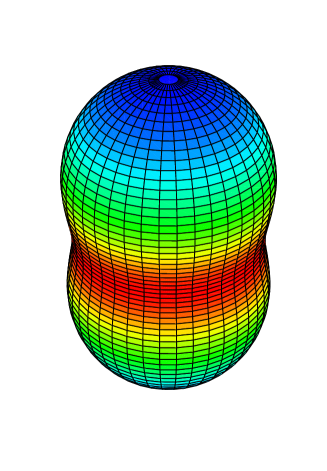
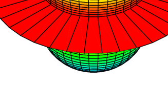
Figure 2.: Left: Iso-mass loss distribution for a 120 M_⊙ star with $\log{\frac{L}{L_{\odot}}=6.0}$ and T${}_{\mathrm{eff}}=30000$ K rotating at a fraction 0.80 of break–up velocity. Right: The same with T${}_{\mathrm{eff}}=25000$ K, (Maeder & Desjacques 2000).

The theory of radiative winds applied to a rotating star leads to an expression (Maeder 1999) of the mass flux as a function of colatitude. Figs. 2 illustrate the distribution of the mass loss rates around a massive star of 120 M_⊙ with two different $T_{\mathrm{eff}}$. For a star hot enough to have electron scattering opacity as the dominant opacity source from pole to equator, the iso–mass loss curve has a peanut–like shape (Fig. 2 left). This results from the fact that the pole is hotter (“$g_{\mathrm{eff}}$–effect”). If the $T_{\mathrm{eff}}$ of the star is lower, a bistability limit (i.e. a steep increase of the opacity, cf. Lamers 1995) may occur somewhere between the pole and the equator, due to the decrase of $T_{\mathrm{eff}}$ from pole to equator. This “opacity–effect” produces an equatorial enhancement of the mass loss (Fig. 2 right). The anisotropies of mass loss influence the loss of angular momentum, in particular polar mass loss removes mass but relatively little angular momentum. This may strongly influence the evolution (Maeder 2002; see Fig. 5 left below). We may estimate the mass loss rates of a rotating star compared to that of a non–rotating star at the same location in the HR diagram. The result is (Maeder & Meynet 2000)

$$\frac{\dot{M}(\Omega)}{\dot{M}(0)}\simeq\frac{\left(1-\Gamma\right)^{\frac{1}{\alpha}-1}}{\left[1-\frac{4}{9}(\frac{v}{v_{\mathrm{crit,1}}})^{2}-\Gamma\right]^{\frac{1}{\alpha}-1}}\;,$$ (8)

where $\Gamma$ is the electron scattering opacity for a non–rotating star with the same mass and luminosity, $\alpha$ is a force multiplier (Lamers et al. 1995). Values of $\alpha$ are given in Table 1, which shows, for stars of different masses and $\Gamma$, the values of the ratio of the mass loss rates for a star at critical rotation to that of a non–rotating star of the same M, L and $T_{\mathrm{eff}}$.

Figure 3.: Left: Evolution during the MS phase of the angular velocity in the interior of a 20 M_⊙ star at $Z$=0.02. Right: the same for a 15 M_⊙ star at $Z=10^{-5}$. The values of the central H–content $X_{\mathrm{c}}$ are indicated. (From Meynet & Maeder 2000, 2002).

The values $\infty$ indicate that the critical velocity $v_{\mathrm{crit,2}}$ is met. Close to $\Gamma=1$ the increase of the mass loss rates may be quite large. For blue and red supergiants, the increase could also be large, however supergiants do not rotate very fast in general.

We must distinguish 3 cases of stellar break–up: 1.– The $\Gamma$–Limit, when radiation effects largely dominate; 2.– The $\Omega$–Limit, when rotation effects are essentially determining break–up and 3.– The $\Omega\Gamma$–Limit, when both rotation and radiation are important for the critical velocity and Eq. (8) applies. For very massive stars, the $\Omega\Gamma$–Limit is clearly the relevant case.

Table 1.: Values of $\frac{\dot{M}(\Omega)}{\dot{M}(0)}$ for different stellar masses. The four force multipliers $\alpha$ apply respectively to stars with: $4.70\geq\log T_{\mathrm{eff}}\geq 4.35$ (type B1.5 or earlier), $\log T_{\mathrm{eff}}$ = 4.30 (type B2.5), 4.00 (B9.5), 3.90 (A7) respectively.

$M_{\rm ini}$	$\Gamma$	$\frac{\dot{M}(\Omega)}{\dot{M}(0)}$	$\frac{\dot{M}(\Omega)}{\dot{M}(0)}$	$\frac{\dot{M}(\Omega)}{\dot{M}(0)}$	$\frac{\dot{M}(\Omega)}{\dot{M}(0)}$
		$\alpha$ = 0.52	$\alpha$ = 0.24	$\alpha$ = 0.17	$\alpha$ = 0.15
120	0.903	$\infty$	$\infty$	$\infty$	$\infty$
85	0.691	$\infty$	$\infty$	$\infty$	$\infty$
60	0.527	3.78	96.2	1130	3526
40	0.356	2.14	13.6	55.3	106.0
25	0.214	1.76	7.02	20.1	32.6
20	0.156	1.67	5.87	15.2	23.6
15	0.097	1.60	5.04	12.1	18.1
12	0.063	1.57	4.68	10.8	15.8
9	0.034	1.54	4.41	9.8	14.2

3. Evolution of rotational velocities

Fig. 3 shows the evolution during the MS phase of the internal angular velocities in models at $Z=0.02$ (left) and at $Z=10^{-5}$ (right). We see that the decrease of the core rotation is stronger at higher $Z$. This is due to the larger mass loss which removes more angular momentum, (the case of isotropic mass loss is considered here with Eq. (8) above). We note that the gradient of $\Omega$ built during MS evolution outside the core is larger at lower $Z$. There are 2 reasons for that. One is the higher compactness of the star at lower $Z$. The second one is more subtle. At $Z=0.02$, the density of the outer layers is lower and the star is more extended than at lower $Z$, thus the Gratton–Öpik term is more important. This produces an outward transport of angular momentum and smoothens the $\Omega$–gradient at $Z=0.02$ more than at lower $Z$. The steeper $\Omega$–gradient at lower $Z$ is leading to stronger mixing of chemical elements, as shown below.

Figure 4.: Evolution of the equatorial velocities along the redward parts of the tracks in the HR diagram for initial velocities of 300 km s^-1 and $Z=0.02$, (Meynet & Maeder 2000).

The evolution of the surface velocities results from internal transport and surface losses of angular momentum. Fig. 1 (right) shows the evolution of the surface velocities for a 60 M_⊙ model for 3 very different metallicities $Z$. For such a large mass, the high losses of mass and angular momentum lead to a strong decrease of rotation at $Z=0.02$. On the contrary, at lower $Z$ the velocities are growing, as a result of the contraction of the stellar core and of the relatively good coupling of the outer layers produced by circulation. Thus, it is likely that at low $Z$, rotation may be a dominant effect in massive star evolution. These stars may reach break–up and then loose a significant amount of matter. Paradoxically, low $Z$ stars may loose mass due to fast rotation as a consequence of their initial slow winds!

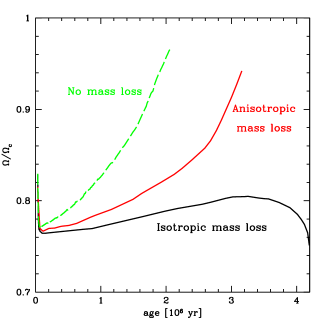
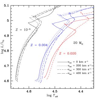
Figure 5.: Left: Evolution of the ratio $\frac{\Omega}{\Omega_{\mathrm{c}}}$ of the angular velocity to the critical value during the MS phase of a 40 M_⊙ star with an initial velocity of 500 km s^-1 (Maeder 2002). Right: Evolutionary tracks on the MS for 20 M_⊙ models of different $Z$ and initial velocities $v_{\mathrm{ini}}$, (Meynet & Maeder 2002).

In addition, we may wonder whether the initial distribution of stellar rotation velocities is the same at lower $Z$. There are some reasons (Maeder et al. 1999) to suspect that the initial rotation velocities may be faster at lower $Z$.

Fig. 4 shows the lines of iso–rotational velocities in the HR diagram of massive stars at $Z=0.02$ for an initial velocity of 300 km/s. We see an important decrease for the most massive stars. This provides the basis for interesting comparison tests. Let us emphasize that the decline will be less important when the anisotropic losses of angular momentum are accounted for, which is not the case in Fig. 4. Fig. 5 (left) shows the very different evolution of the surface rotation of fast rotating stars for different cases of mass loss. For zero–mass loss, critical velocities are reached very quickly. For isotropic mass loss (here the relatively lower rates by Vink et al. 2001), there is no increase of $\frac{\Omega}{\Omega_{\mathrm{c}}}$. The case with account of the anisotropic losses of angular momentum gives results intermediate between the two previous cases, with some significant increase of $\frac{\Omega}{\Omega_{\mathrm{c}}}$. If there is some magnetic coupling, $\frac{\Omega}{\Omega_{\mathrm{c}}}$ will be larger during evolution. Thus, the study of rotational velocities for stars at various distances from the ZAMS may provide a powerful test on the role of magnetic field.

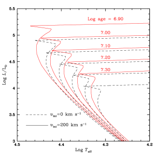
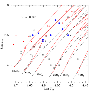
Figure 6.: Left: Isochrones with and without rotation for solar metallicity. Right: Evolutionary tracks in the log g_eff vs. log T_eff diagram. The dashed lines correspond to non–rotating tracks, the continuous lines are for models with an initial rotation of 300 km s^-1. The small dotted line corresponds to a very fast rotating 60 M_⊙. The observations are by Herrero et al. (2000) and previous works.

4. HR diagram, lifetimes and isochrones

Table 2 provides various information on the effects of rotation for a 20 M_⊙ star. We show the average velocities during the MS phase, the MS lifetimes, the masses and velocities at the end of the MS, the helium content, the N/C and N/O ratios at the end of the MS. We notice the growth of the MS lifetimes for higher rotation velocities, as well as the lower final masses. This results from both the longer MS lifetimes and from the higher mass loss rates. We notice the chemical enrichments at the stellar surface. Some isochrones calculated for initial velocities $v_{\mathrm{ini}}=200$ km/s are displayed in Fig. 6 (left); these $v_{\mathrm{ini}}$ lead to average velocities on the MS of about 140 km/s. If we assign cluster ages from these isochrones, we obtain ages typically 25% larger than from the standard models without rotation. For average velocities of about 220 km/s, the difference on the age estimate would be larger. This effect may easily help us to reconcile the ages for the Pleiades determined from the turnoff with the ages from lithium abundances in the low mass stars of the Pleiades (Martin et al. 1998).

Table 2.: Properties of 20 M_⊙ models at the end of the MS for different initial velocities. The velocities are in km s^-1, the lifetimes in million years, the masses in solar mass and the surface abundances in mass fraction.

$v_{\rm ini}$	$\overline{v}$	$t_{H}$	M	$v$	He	N/C	N/O
0	0	7.350	19.019	0	0.30	0.25	0.12
50	30	7.720	18.896	18	0.30	0.27	0.12
100	62	8.292	18.681	46	0.30	0.45	0.19
200	132	8.901	18.324	94	0.32	1.01	0.38
300	197	9.309	18.020	167	0.35	1.77	0.58
400	253	9.745	17.646	217	0.37	2.54	0.76
500	294	10.275	17.181	213	0.40	3.65	0.99
580	304	10.324	17.148	214	0.39	3.75	1.00

Fig. 6 (right) shows the tracks in the $\log g_{\mathrm{eff}}$ vs. $\log T_{\mathrm{eff}}$ plot.We see that if we assign an evolutionary mass to a rotating star on the basis of a track without rotation, we obtain a mass which may be up to a factor of 2 too large. Appropriate tracks have to be used for rotating stars. The non–respect of this prescription is likely the explanation of the so–called problem of the mass discrepancy.

5. Surface abundances

Figure 7.: Left: Evolution as a function of $logT_{\mathrm{eff}}$ of the abundance ratio N/C (in number), normalized to their initial values. The tracks are for $Z=0.004$. A model at Z=0.02 is also shown. The track with 0 km/s applies to both $Z=0.020$ and $Z=0.004$. Right: Evolution of $T_{\mathrm{eff}}$ as a function of the fraction of lifetime spent in the He–burning phase fo 15, 20 and 25 M_⊙ at $Z=0.004$ for $v_{\mathrm{ini}}=0$ and 300 km/s, (Maeder & Meynet 2001).

As a result of internal mixing, He and N are brought to the surface, while C is depleted. At solar $Z$, the N/C ratios are increased by a factor 2–3 for a 20 M_⊙ model (Fig. 7 left). For lower $Z$, we see that the enrichment in N/C is much larger. This results from the larger shears in low metallicity models (Fig. 3). The higher N–enhancements at lower $Z$ are consistent with the results by Venn (1998, 1999), who has found excesses of N/H up to about a factor of 10 in supergiants of the SMC. At $Z=0.004$, the models show no sign of primary nitrogen. Models at $Z=10^{-5}$ by Meynet & Maeder (2002) show large amounts of primary nitrogen, which change the sum of CNO elements in advanced stages.

There is still a problem (Herrero et al. 2000). There are many fast rotating stars, which have He excesses. The models indicate that when the products of CNO burning appear at the surface, the velocities have already significantly decreased. A possible explanation is that there are initially many very fast rotating stars, where the enrichments appear quickly. Also, nuclear reactions in massive stars are active in the pre–MS phase and thus mixing may already occur during the pre–MS phase.

6. The blue to red supergiant ratio

In clusters of low $Z$, as in the SMC, there are lots of red supergiants. However, the models of massive stars at low $Z$ do not reach in general the red stage. If they do it, this happens only very late in evolution, so that there are no red supergiants predicted. Fig. 7 (right) illustrates the point: for zero rotation most of the He–burning phase is spent in the blue and very little in the red.

Rotation very much changes the above results. Fig. 7 (right) shows that the models of 15 to 25 M_⊙ with rotation spend at least half of the He-burning lifetime in the red. This is in agreement with the blue to red supergiant ratios of 0.5–0.8 observed in the SMC. The physical reason why rotation makes more red supergiants is the following one: with rotation, the He–burning core is larger and there are also more He mixed just outside the core, in particular at the location of the H–burning shell. Since the core is larger, and as there is also more He outside, the H–shell is less active and the opacity is also lower. Thus, while there is an intermediate convective zone in non–rotating models, there is none in models with rotation. Convection means a polytropic index $n=1.5$ and thus a high degree of compactness, which keeps the non–rotating stars in the blue. With rotation, the absence of intermediate convective zone permits the envelope to largely expand and the star moves toward the red supergiant stage.

On the whole, we see that rotation is an essential ingredient of stellar models and that rotation modifies all the model outputs.

Acknowledgements: We express our thanks to Raphael Hirschi for a careful reading of the manuscript.

References

Chaboyer, B., Zahn, J.P. 1992, A&A 253, 173

Herrero, A., Puls, J., Villamariz, M.R. 2000, A&A 354, 193

Kippenhahn, R., Thomas, H.C. 1970, in Stellar Rotation, IAU Coll. 4, Ed. A. Slettebak, Gordon and Breach, p. 20

Lamers, H.J.G.L.M., Snow, T.P., Lindholm, D.M. 1995, ApJ 455, 269

Maeder, A. 1999, A&A 321, 134 (paper II)

Maeder, A. 1999, A&A 347, 185 (paper IV)

Maeder, A. 2002, A&A 392, 575 (paper IX)

Maeder, A., Desjacques, V. 2000, A&A 372, L9

Maeder, A., Grebel, E. & Mermilliod, J.-C. 1999, A&A 346, 459

Maeder A., Meynet G. 2000, A&A 361, 159 (paper VI)

Maeder A., Meynet G. 2001, A&A 373, 555 (paper VII)

Maeder A., Peytremann, E. A&A, 7, 120

Maeder A., Zahn J.P. 1998, A&A, 334, 1000 (paper III)

Martin, E.L., Basri, G., Gallegos, J.E. et al. 1998, Ap.J. 499, L61

Meynet G., Maeder A. 1997, A&A, 321, 465 (paper I)

Meynet G., Maeder A. 2000, A&A, 3, 101 (paper V)

Meynet G., Maeder A. 2002, A&A, 390, 561 (paper VIII)

Talon, S., Zahn, J.P. 1997, A&A 317, 749

Venn, K.A. 1998, in Boulder–Munich II: Properties of Hot Luminous Stars, ed. I. Howarth, ASP Conf. Ser., 131, 177

Venn, K.A. 1999, ApJ 518, 405

Vink, J.S., de Koter, A. & Lamers, H.J.G.L.M. 2001, A& A 362, 295

Walborn, N. 1976, ApJ, 205, 419

Zahn J.P. 1992, A&A 265, 115