Stellar rotation: Evidence for a large horizontal turbulence and its effects on evolution

We derive a new expression for the coefficient $D_{\mathrm{h}}$ of diffusion by horizontal turbulence in rotating stars. This new estimate can be up to two orders of magnitude larger than given by a previous expression. As a consequence the differential rotation on an equipotential is found to be very small, which reinforces Zahn’s hypothesis of shellular rotation. The role of the so–called $\mu$–currents, as well as the driving of circulation, are reduced by the large horizontal turbulence. Stellar evolutionary models for a 20 M${\odot}$ star are calculated with the new coefficient. The new and large $D_{\mathrm{h}}$ tends to limit the size of the convective core and at the same time it largely favours the diffusion of helium and nitrogen to the surface of rotating OB stars, a feature supported by recent observations. hysical data and processes: turbulence – Stars: evolution – Stars: rotation

1 Introduction

Differential rotation usually creates turbulent motions due to shear in rotating stars. In a normally stable radiative layer, the turbulence is usually much stronger in the horizontal direction perpendicular to gravity than in the vertical direction (Zahn Zahn92 (1992)). The reason is that in the vertical direction the stable temperature gradient needs stronger forces to be overcome than in the horizontal direction where, in principle, no forces are opposed to the motions. An argument in favour of these intense horizontal meteorological–like turbulent motions is given by the study of the solar tachocline by Spiegel & Zahn (spiegzahn92 (1992)). The tachocline is the transition zone between the rigid rotation in the radiative interior and the external convective zone, where rotation varies with latitude. Spiegel & Zahn show that if the horizontal turbulence is intense, then the tachocline is very thin as supported by helioseismological observations.

The global result of the transport of the fluid elements by the horizontal turbulence is represented by a coefficient of viscosity $\nu_{\mathrm{h}}$. This coefficient is a very important parameter in the physics of rotating stars in several respects:

–1. If strong enough, the horizontal coupling expressed by the coefficient $\nu_{\mathrm{h}}$ makes the angular velocity $\Omega$ nearly constant on isobaric surfaces (cf. Zahn Zahn92 (1992)). In this case, the angular velocity $\Omega$ is constant on shells and the rotation law is said “shellular” by Zahn. If this is the case, the equations of stellar structure are greatly simplified, because they depend on one coordinate only (which is not just the lagrangian coordinate M_r, but which has to be defined in an appropriate way). This enables us to keep a 1–D equations scheme for stellar structure (cf. Kippenhahn & Thomas kipp70 (1970); Endal & Sofia endsof76 (1976)). In the case of differential shellular rotation, Meynet & Maeder (MMI (2000)) have shown that the scheme usually employed is incorrect, but that a consistent 1–D scheme may still be defined.

–2. The various mixing processes of chemical elements play a major role in massive star evolution (cf. Heger et al. heger1 (2000); Heger & Langer heger2 (2000); Meynet & Maeder MMI (2000)). The horizontal turbulence reduces very much the efficiency of vertical transport of elements by meridional circulation (Chaboyer & Zahn chabzahn92 (1992)). This enables us to understand in a consistent way why the vertical transport of chemical elements by the circulation is much smaller than the vertical transport of angular momentum by circulation. This is a clear constraint which results from solar observations (Chaboyer et al. 1995a ; 1995b ), as well as from the observations of massive stars (Maeder & Meynet MMI (2000)).

–3. The horizontal turbulence was generally ignored in the treatment of meridional circulation or of shear mixing. However, recent developments (Chaboyer & Zahn chabzahn92 (1992); Maeder & Zahn MZIII (1998); Maeder & Meynet MMVII (2001); Brüggen & Hillebrandt bruggen (2001)) show that the horizontal diffusion by turbulence may also intervene in the expressions of the transport of chemical elements by meridional circulation, of the circulation velocity, of the diffusion coefficient by shear mixing, of the heat transport, etc… Interestingly enough, the numerical convergence of the 4th order scheme of differential equations expressing the transport of angular momentum and meridional circulation appears to be sensitive to the value of diffusion coefficient of horizontal turbulence.

We do not consider here the effect of the magnetic field (cf. Spruit spruit (2002)), which may also play a role in the transport of angular momentum. In Sect.2, we examine the reasons which demand a new estimate of $\nu_{\mathrm{h}}$. In Sect. 3, we derive a new expression for $\nu_{\mathrm{h}}$ and some numerical estimates. Sect. 4 provides a discussion of the results.

2 Reasons for a new estimate of the horizontal turbulence

The usual expression for the coefficient $\nu_{\mathrm{h}}$ of viscosity due to horizontal turbulence and for the coeffcient $D_{\mathrm{h}}$ of horizontal diffusion, which is of the same order, is, according to Zahn (Zahn92 (1992); Eq.(2.29)),

$$D_{\mathrm{h}}\simeq\nu_{\mathrm{h}}=\frac{1}{c_{\mathrm{h}}}r\;|2V(r)-\alpha U(r)|\,\,,$$ (1)

where $r$ is the appropriately defined eulerian coordinate of the isobar (Meynet & Maeder MMI (2000)). Apart from the case of extreme rotational velocities, the parameter $r$ is close to the average radius of an isobar, which is the radius at $P_{2}(\cos\vartheta)=0$, namely for $\vartheta=54.7$ degrees. $U(r)$ is the vertical component of the velocity of meridional circulation, $V(r)$ the horizontal component, $\alpha=\frac{1}{2}\frac{d\ln r^{2}\overline{\Omega}}{d\ln r}$ and $c_{\mathrm{h}}$ is a constant of order of unity or smaller. This equation was derived assuming that the differential rotation (as defined by the ratio $\frac{\Omega_{2}(r)}{\overline{\Omega}(r)}$ in Eq.(4) below) on an isobaric surface be small compared to unity. Indeed, there are several difficulties suggesting us to reconsider the expression for $\nu_{\mathrm{h}}$:

– The first reason why the above expression is not satisfactory has been given by Zahn (Zahn92 (1992)) and it is related to the way Eq.(1) has been obtained. If we write the differential rotation at a colatitude $\vartheta$ as

$$\Omega(r,\vartheta)=\overline{\Omega}(r)+\widehat{\Omega}(r,\vartheta)\quad\mathrm{with}$$ (2)

$$\widehat{\Omega}(r,\vartheta)=\Omega_{2}(r)\,P_{2}(\cos\vartheta)\,,$$ (3)

where $P_{2}(\cos\vartheta)$ is the Legendre polynomial of second order, we find that the differential rotation is a constant (cf. Sect. 2.6 in Zahn Zahn92 (1992)),

$$\frac{\Omega_{2}(r)}{\overline{\Omega}(r)}=\frac{c_{h}}{5}\,.$$ (4)

This ratio is obtained when we use a coefficient $\nu_{\mathrm{h}}$ given by Eq.(1) together with the expressions for the horizontal transport of angular momentum. This ratio is smaller than unity, but, as noted by Zahn (Zahn92 (1992)), there is no reason for the amount of differential rotation being constant with $r$. On the contrary, the importance of differential rotation should depend on the value of $\nu_{\mathrm{h}}$, because the stronger the horizontal turbulence, the stronger is the homogeneisation of the angular velocity on an equipotential surface. This suggests that $\frac{\Omega_{2}(r)}{\overline{\Omega}(r)}$ should decrease for larger $\nu_{\mathrm{h}}$. Likely, we could also expect that the importance of differential rotation varies with the rotation velocity, since the horizontal turbulence is itself generated by rotation.

– Another point is related to the numerical models (Meynet & Maeder, MMV (2000); Maeder & Meynet, MMVII (2001)). During the course of the evolution, some models indicate that the coefficient $D_{\mathrm{h}}$ of horizontal turbulence, as given by Eq.(1), is not so much larger than the coefficient of vertical diffusion by shear, especially at low metallicity $Z$ where $U(r)$ is small (see Fig. 6 in Meynet & Maeder MMV (2000) and Fig. 2 in Maeder & Meynet MMVII (2001)). This is not very satisfactory for the validity of the assumption of shellular rotation. We may remark in this context that this assumption would be much better if the diffusion coefficient of horizontal turbulence would be larger.

– We may also note that physically the horizontal turbulence results from the differential rotation, while the meridional circulation with components $U(r)$ and $V(r)$ results from the disruption of the thermal equilibrium on an equipotential. These two phenomena are generally, but not necessarily, related. An example is the case of a uniformly rotating star. There we have no differential rotation, but a breakdown of thermal equilibrium occurs unavoidably.

3 The dissipation and feeding of turbulent energy

Let us firstly examine the rate of dissipation of the turbulent energy. As shown by Zahn (Zahn92 (1992)), we may write the rate of viscous dissipation of the energy present in the differential zonal motions on an isobar as

$$\delta\dot{\epsilon}_{\mathrm{t}}(r,\vartheta)=\nu_{\mathrm{h}}\left(\sin\vartheta\,\frac{\partial\widehat{\Omega}}{\partial\vartheta}\;\delta\vartheta\right)^{2}\;,$$ (5)

per mass and time and for an interval of latitude $\delta\vartheta$. Taking into account Eq.(3), we obtain

$$\delta\dot{\epsilon}_{\mathrm{t}}(r,\vartheta)=\nu_{\mathrm{h}}\sin^{2}\vartheta\;\Omega_{2}^{2}(r)\left(\frac{dP_{2}(\cos\vartheta)}{d\vartheta}\right)^{2}\delta\vartheta^{2}\;,$$ (6)

$$\delta\dot{\epsilon}_{\mathrm{t}}(r,\vartheta)=9\;\nu_{\mathrm{h}}\;\Omega_{2}^{2}(r)\sin^{4}\vartheta\cos^{2}\vartheta\delta\vartheta^{2}\;.$$ (7)

The rate of energy dissipation is proportional to the square of the amplitude $\Omega_{2}(r)$ on an equipotential. It is zero at the pole and equator and maximum at $P_{2}(\cos\vartheta)=0$.

There is an excess of energy on an isobar due to the differential rotation described by Eq.(2) compared to an average rotation. The velocity of rotation $v(r,\vartheta)$ on the equipotential of average distance $r$ is given by

$$v(r,\vartheta)=r\,\sin\vartheta\overline{\Omega}+r\;\sin\vartheta\Omega_{2}(r)\;P_{2}(\cos\vartheta)\;.$$ (8)

For an interval of latitude $\delta\vartheta$, the difference of rotational velocity $\delta v(r,\vartheta)$ due to the latitudinal differential rotation on the equipotential is

$$\delta v(r,\vartheta)=r\,\sin\vartheta\;\Omega_{2}(r)\frac{dP_{2}(\cos\vartheta)}{d\vartheta}\delta\vartheta$$

$$=-3r\;\sin^{2}\vartheta\cos\vartheta\;\Omega_{2}(r)\delta\vartheta.$$ (9)

We express here only in the velocity difference due to the shear on the equipotential. The excess of energy $\delta E_{\mathrm{diff}}(r,\vartheta)$ over an interval $\delta\vartheta$ due to the differential rotation in latitude is

$$\delta E_{\mathrm{diff}}(r,\vartheta)=\frac{1}{4}\,\delta v^{2}(r,\vartheta)$$

$$=\frac{9}{4}\,r^{2}\sin^{4}\vartheta\cos^{2}\vartheta\;\Omega^{2}_{2}(r)\;\delta\vartheta^{2}.$$ (10)

Now, this small excess of energy over an interval $\delta\vartheta$ will be smeared out in a dynamical timescale $\delta t_{\mathrm{diff}}$.

Let us estimate this characteristic timescale. On the isobar, the differential rotation due to $\Omega_{2}$ produces a shift $\delta\varphi$ in longitude for two fluid elements located at a difference $\delta\vartheta$ in colatitude in a time interval $\delta t$

$$\delta\varphi=\delta\widehat{\Omega}\,\delta t=\Omega_{2}{dP_{2}\over d\vartheta}\;\delta\vartheta\,\delta t\;.$$ (11)

The meridional circulation has an horizontal velocity component ${V}$, which is pointing toward the pole in the external layers where $U(r)<0$. This is due to the Gratton–Öpik term, which is the term $-\frac{\overline{\Omega^{2}}}{2\pi G\overline{\rho}}$ (Öpik op (1951)) which appears in the equation for $U(r)$ given for example in Eq.(4.29) by Maeder & Zahn (MZIII (1998)). Due to the average density $\overline{\rho}$ at the denominator, the Gratton–Öpik term is largely negative near the surface, thus it acts so as to change the sign of the circulation $U(r)$, making it rising in the equatorial plane and descending along the polar axis. In the deeper layers, one has generally $U(r)>0$, which means that the circulation rises along the polar axis and descends in the equatorial plane. Thus, in this case $V$ is pointing toward the equator. The shift in latitude is given by

$$r\;\delta\vartheta=V{dP_{2}\over d\vartheta}\;\delta t\;,$$ (12)

and this leads to

$$\delta\varphi={\Omega_{2}V\over r}\left({dP_{2}\over d\vartheta}\right)^{2}(\delta t)^{2}.$$ (13)

The complex motion in $\vartheta$ and $\varphi$ due to the differential rotation $\Omega_{2}$ on the isobar will tend to smear out the latitudinal energy differences as discussed above. As a typical dynamical timescale, we take the time necessary for this differential motion in $\varphi$ to perform $n$ axial rotations. We may consider an average of $\delta\varphi(\vartheta)$ over the star

$$\overline{\delta\varphi}={\Omega_{2}V\over r}\;(t_{\mathrm{diff}})^{2}\int^{\pi\over 2}_{0}\left({dP_{2}\over d\vartheta}\right)^{2}\sin{\vartheta}\;d\vartheta\;=2n\pi\;.$$ (14)

Thus, we get for the characteristic timescale

$$t_{\rm diff}=\left(\frac{5n\pi}{3}{r\over\Omega_{2}V}\right)^{1/2}\;.$$ (15)

The numerical factor is of course rather arbitrary. The ratio of the energy excess (Eq.(10)) and of the rate of viscous dissipation (Eq.(7)) is of the order of this timescale and we write

$$\frac{\delta E_{\mathrm{diff}}(r,\vartheta)}{\delta\dot{\epsilon}_{\mathrm{t}}(r,\vartheta)}=\;t_{\rm diff}\;.$$ (16)

Using Eqs.(7) and (10), we obtain for the coefficient of horizontal turbulence $\nu_{\mathrm{h}}$

$$\nu_{\mathrm{h}}=\left(\frac{3}{80n\pi}\;r^{3}\Omega_{2}V\right)^{\frac{1}{2}}\;.$$ (17)

We may also estimate $\nu_{\mathrm{h}}$ by dividing the square of a typical lengthscale (of the order of $r$) by the diffusion timescale given by Eq.(15). We obtain exactly the same functional dependence in $(r^{3}\Omega_{2}V)^{1\over 2}$, with a numerical coefficient depending on the chosen lengthscale. Studying conservation of the angular momentum by taking into account the horizontal variations $\Omega_{2}$ of rotation leads to the following relation (Zahn Zahn92 (1992); Eq.(2.27)), that relates $\Omega_{2}$ and $\nu_{\mathrm{h}}$

$$\nu_{\mathrm{h}}\;\Omega_{2}(r)=\frac{1}{5}\;\overline{\Omega}(r)\;r\left[2V-\alpha U\right]\;,$$ (18)

where $\alpha$ is the same as in Eq.(1). This is the expression discussed in Sect. 2 , which implies that, if $\nu_{\mathrm{h}}$ is given by an equation like Eq.(1), the ratio $\frac{\Omega_{2}}{\overline{\Omega}(r)}$ is a constant. Now, we eliminate $\Omega_{2}$ between the two equations (17) and (18). This gives for the coefficient of viscosity due to the horizontal turbulence

$$\nu_{\mathrm{h}}=A\;r\;\left(r\overline{\Omega}(r)\;V\;\left[2V-\alpha U\right]\right)^{\frac{1}{3}}$$

$$\mathrm{with}\quad A=\left(\frac{3}{400n\pi}\right)^{\frac{1}{3}}\;.$$ (19)

For n=1, 3 or 5 $A\approx 0.134,0.0927,0.0782$ respectively. This expression can be written in the usual form $\nu_{\mathrm{h}}=\frac{1}{3}\;l\cdot v$ for a viscosity, where the appropriate velocity $v$ is a geometric mean of 3 relevant velocities:

• A velocity $(2V-\alpha U)$ as in Eq.(1) by Zahn (Zahn92 (1992)),

• The horizontal component $V$ of the meridional circulation.

• The average local rotational velocity $r\overline{\Omega}(r)$. This rotational velocity is usually much larger than either $U(r)$ or $V(r)$, typically by 6 to 8 orders of a magnitude in an upper Main Sequence star rotating with the average velocity.

4 Numerical results

4.1 Comparisons and orders of magnitude

Let us compare the present value of $\nu_{\mathrm{h}}$ to that given by Zahn (Zahn92 (1992)). We get the following ratio from Eq.(1) and (19),

$$\frac{\nu_{\mathrm{h}}(present)}{\nu_{\mathrm{h}}(Zahn)}=\;A\,c_{\mathrm{h}}\left({\frac{r\;\overline{\Omega}\;V}{(2V-\alpha U)^{2}}}\right)^{\frac{1}{3}}\;.$$ (20)

The quantities $V$ and $U$ have the same order of magnitude. The numerical models below show that typically $V\approx\frac{1}{3}U$ and $(2V-\alpha U)\approx V$, thus we have the following order of magnitude,

$$\frac{\nu_{\mathrm{h}}(present)}{\nu_{\mathrm{h}}(Zahn)}\approx\;A\,c_{\mathrm{h}}\left(\frac{r\;\overline{\Omega}}{V}\right)^{\frac{1}{3}}\;.$$ (21)

Thus, we see that the ratio of the two estimates of the diffusion coefficient is equal to the power $\frac{1}{3}$ of the ratio of the local rotational velocity to the horizontal velocity of meridional circulation at the considered level. Let us consider a 20 M_⊙ star with an average rotation velocity of 220 km/s at the surface. At the middle of the MS phase, the vertical component of the meridional circulation lies between $3\cdot 10^{-4}$ and $3\cdot 10^{-3}$ m/s as shown by the models below (see also Meynet & Maeder MMV (2000)). Thus, we typically have $\frac{\nu_{\mathrm{h}}(present)}{\nu_{\mathrm{h}}(Zahn)}$ of the order of $10^{2}$ (cf. Fig. 1). Thus, our estimate of the diffusion coefficient of the horizontal turbulence is much larger than the coefficient proposed by Zahn(Zahn92 (1992); Eq.(2.29)) as given by Eq.(1).

Let us now estimate the degree of differential rotation corresponding to this value of $\nu_{\mathrm{h}}$. From Eq.(18), we have with Eq.(19),

$$\frac{\Omega_{2}}{\overline{\Omega}(r)}=\frac{1}{5\;A}\left(\frac{(2V-\alpha U)^{2}}{r\;\overline{\Omega}V}\right)^{\frac{1}{3}}$$ (22)

There is of course no coefficient $c_{\mathrm{h}}$ in this ratio. Numerically, this is 1/5 of the inverse of the ratio given by Eq.(20), in which the value of $c_{\mathrm{h}}=1$ would be used. This results from Eq.(1) and Eq.(18) relating $\nu_{\mathrm{h}}$ and $\Omega_{2}$. Thus, with the above estimates, we obtain a ratio of about $\frac{\Omega_{2}}{\overline{\Omega}(r)}=2\cdot 10^{-3}$. As the value of $\nu_{\mathrm{h}}$ obtained in this work is much larger than the value given by Eq.(1), we see that quite logically the degree of differential rotation on an isobar is much smaller. The present value of the coefficient reinforces Zahn’s hypothesis of shellular rotation. We also notice that the ratio $\frac{\Omega_{2}}{\overline{\Omega}(r)}$ is larger for slowly rotating stars. This is quite a consistent feature, because $\nu_{\mathrm{h}}$ is growing with the velocity of rotation.

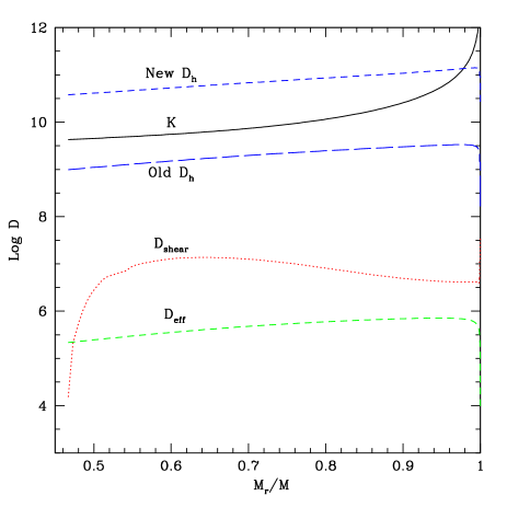
Figure 1: Values of the various diffusion coefficient in the interior of a star model of 20 M_⊙ at beginning of the MS phase, with an age of $8.577\cdot 10^{4}$ yr. and central hydrogen content of $X_{\mathrm{c}}=0.702$. That is to say during the initial non–stationary phase of convergence of the rotation, where the velocities $U(r)$ are large. The new $D_{\mathrm{h}}$ is that given by Eq.(19) with A=0.079. The old $D_{\mathrm{h}}$ is that given by Eq.(1). $K$ is the radiative diffusivity. $D_{\mathrm{shear}}$ is the coefficient of diffusion by shears. $D_{\mathrm{eff}}$ expresses the diffusion of the chemical elements by meridional circulation with account of the effects of horizontal turbulence. When not specified, the quantities shown are those for the new $D_{\mathrm{h}}$.

4.2 Test with the evolution of a 20 M_⊙ model

In order to examine the consequence of the new coefficient of horizontal diffusion, we calculate stellar models for a 20 M_⊙ with composition $X=0.705$ and $Z=0.02$ with the same physics as in our recent papers (Maeder & Meynet MMVII (2001)). The initial rotation velocity is 300 km/s, which corresponds to average rotation during the MS phase of about 240 km/s. Several expressions and diffusion coefficients will be discussed numerically below, let us briefly recall them. The vertical component $U(r)$ of the velocity of meridional circulation velocity is given by

$${U(r)=\frac{P}{{\rho}{g}C_{\!P}{T}\,[\nabla_{\rm ad}-\nabla+(\varphi/\delta)\nabla_{\mu}]}}\;\times$$

$$\left\{\frac{L}{M_{\star}}(E_{\Omega}+E_{\mu})\right\}\;.$$ (23)

P is the pressure, $C_{P}$ the specific heat, $E_{\Omega}$ and $E_{\mu}$ are terms depending on the $\Omega$– and $\mu$–distributions respectively, up to the third order derivatives and on various thermodynamic quantities (see details in Maeder & Zahn, MZIII (1998)). The term $E_{\Omega}$ expresses the driving effects of meridional circulation, while the term $E_{\mu}$ expresses the $\mu$–currents which tend to inhibit the circulation. The term $\nabla_{\mu}$ is very important numerically, its origin in this expression is more complex than could be thought at first sight. This expression also prevents infinite velocities at the edge of semiconvective zones. The term $E_{\Omega}$ expresses the driving of the circulation by the fluctuations of density due to the breakdown of radiative equilibrium.

The diffusion by shear instabilities is expressed by a coefficient $D_{\mathrm{shear}}$, namely

$$D_{\mathrm{shear}}=\frac{4(K+D_{\mathrm{h}})}{\left[\frac{\varphi}{\delta}\nabla_{\mu}(1+\frac{K}{D_{\mathrm{h}}})+(\nabla_{\mathrm{ad}}-\nabla_{\mathrm{rad}})\right]}\;\times$$

$$\frac{H_{\mathrm{p}}}{g\delta}\;\left[\frac{\alpha}{4}\left(f\Omega{d\ln\Omega\over d\ln r}\right)^{2}-(\nabla^{\prime}-\nabla)\right]\;.$$ (24)

where $f$ is a numerical factor equal to 0.8836, $K$ is the thermal diffusivity and $(\nabla^{\prime}-\nabla)$ expresses the difference between the internal nonadiabatic gradient and the local gradient (Maeder MII (2001)). There is also the coefficient $D_{\mathrm{eff}}$, which expresses the contribution of the meridional circulation and horizontal turbulence to the diffusion of the elements (Zahn Zahn92 (1992)),

$$D_{\mathrm{eff}}=\frac{|r\;U(r)|^{2}}{30D_{\mathrm{h}}}\;,$$ (25)

while the transport of angular momentum by circulation has to be treated explicitely as an advection. More details on these various expressions, on the hypotheses leading to them and on their domain of validity can be found in the given references.

Fig.1 shows the diffusion coefficients at the very beginning of the MS phase. There, the situation is non-stationary during 1-2 % of the MS lifetime, until the rotation has converged toward an equilibrium profile, (in reality a part of this convergence, but probably not the whole, may be achieved during the pre-MS phase). In this temporary stage, $U(r)$ is usually much larger (about a few $10^{-2}$ m s^-1) than later in the course of evolution, where it is only of the order of a few $10^{-3}$ m s^-1 (Meynet & Maeder MMV (2000)). We point out the much larger value of the new $D_{\mathrm{h}}$ with respect to the old one. With the new $D_{\mathrm{h}}$, we see that $D_{\mathrm{eff}}$ is rather small with respect to $D_{\mathrm{shear}}$, while with the old $D_{\mathrm{h}}$, the coefficient $D_{\mathrm{eff}}$ would have been larger than $D_{\mathrm{shear}}$ everywhere, and in particular by several orders of a magnitude close to the core. As to $D_{\mathrm{shear}}$, the effect is opposite, the new $D_{\mathrm{h}}$ makes it bigger since $K$ is replaced by $K+D_{\mathrm{h}}$, when the $\mu$–gradient is small.

Fig.2 shows the various diffusion coefficients near the middle of MS evolution. Interestingly enough, the star shows 3 cells of meridional circulation. At the interfaces located at $M_{\mathrm{r}}\over M$ = 0.535 and 0.950, the nulling of $U(r)$ produces a kink in the curves of $D_{\mathrm{h}}$, $D_{\mathrm{shear}}$ and $D_{\mathrm{eff}}$. The outer cell is the Gratton–Öpik cell, due to the lower density in the outer layers. The main inner cell is the usually dominant cell where $U(r)$ is positive. There the circulation rises along the polar axis and descends in the equatorial plane, (thus bringing angular momentum toward the interior). The third cell close to the core is not a well understood one. It was already present in some curves of Fig. 4 in Meynet & Maeder (MMV (2000)). The velocities here are very small and slighty negative. We interpret this third cell as due to a change of the second derivative of the angular velocity $\Omega$, which influences the expression of $U(r)$ as given by Maeder & Zahn (MZIII (1998)). (We also remark a kick in the curve of $D_{\mathrm{shear}}$ at $M_{\mathrm{r}}\over M$ = 0.41; it is produced by variations of the nearly vertical gradient of $\mu$ in some regions.)

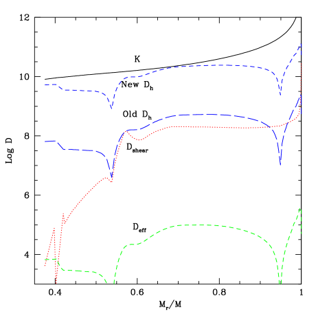
Figure 2: Values of the various diffusion coefficients in the interior of a star model of 20 M_⊙ at about the middle of the MS phase, with an age of $7.066\cdot 10^{6}$ yr. Same remarks about the coefficients of diffusion as in Fig.1.

Fig. 2 tells us a lot about the diffusion coefficients in the stellar interior and their effects:
– As discussed above, the new $D_{\mathrm{h}}$ given by Eq.(19) is larger by about 2 orders of a magnitude with respect to the old one given by Eq.(1), the new value is not far from the thermal diffusivity $K$.
– The new $D_{\mathrm{h}}$ brings some change to $D_{\mathrm{shear}}$. In regions where the $\mu$–gradient is negligible, the ratio $\frac{D_{\mathrm{shear}}(new)}{D_{\mathrm{shear}}(old)}$ of the coefficients of shear diffusion calculated with the new and the old $D_{\mathrm{h}}$ behaves like $\frac{K+D_{\mathrm{h}}}{K}$. In view of the values in Fig. 2, this means that $D_{\mathrm{shear}}$ in the outer regions is increased only moderately, currently less than a factor of two. Comparisons with Fig. 6 by Meynet & Maeder (MMV (2000)) confirms the comparable order of magnitude of $D_{\mathrm{shear}}$.
– When $\nabla_{\mu}>>(\nabla_{\mathrm{ad}}-\nabla_{\mathrm{rad}})$, a situation which occurs close to the convective core, the ratio $\frac{D_{\mathrm{shear}}(new)}{D_{\mathrm{shear}}(old)}$ behaves like $\frac{D_{\mathrm{h}}(new)}{D_{\mathrm{h}}(old)}$. This means that $D_{\mathrm{shear}}$ is increased by a factor of 100 in the internal regions close to the core. Such a change should normally strongly favour mixing in the star, however this is not so much the case, because precisely in the regions close to the core $D_{\mathrm{shear}}$ is very small due to the very steep $\mu$–gradient, which limits the shear diffusion as shown by Eq.(24). Close to the core, $D_{\mathrm{eff}}$ is generally similar or larger than $D_{\mathrm{shear}}$ (this was particularly the case when the low $D_{\mathrm{h}}$ given by Eq.(1) was used).
– Contrarily to the case of $D_{\mathrm{shear}}$, $D_{\mathrm{eff}}$ is reduced by an increase of $D_{\mathrm{h}}$, as is evident from Eq.(25). This can also be seen from a comparison between the present Fig. 2 and Fig. 6 by Meynet & Maeder (MMV (2000)), where much larger values of $D_{\mathrm{eff}}$ can be seen.
– Last but not least, the old $D_{\mathrm{h}}$ was often of the same order as the old $D_{\mathrm{shear}}$ in some parts of the star. This was not satisfactory, in view of the hypothesis of shellular rotation as mentioned in Sect. 2. The new $D_{\mathrm{h}}$, which is much larger than the new $D_{\mathrm{shear}}$ (cf. Fig. 2), solves the problem and makes the hypothesis of shellular rotation a much better one as also indicated by Eq.(22).

Thus we see that a larger horizontal turbulence makes $D_{\mathrm{shear}}$ larger and $D_{\mathrm{eff}}$ smaller. The situation is complex, since the relative importance of these two coefficients is not the same throughout the star. $D_{\mathrm{shear}}$ always dominates at some distance of the stellar core, while $D_{\mathrm{eff}}$ tends to dominate near the core, especially if $D_{\mathrm{h}}$ is small. In addition, the ratio of these two coefficients is changing during evolution, as seen from Fig. 1 and Fig. 2. Thus, a change of $D_{\mathrm{h}}$ affects the evolution of a star in a complex way. These new results now seem kind of very similar to Heger et al. (heger1 (2000)). In a rough summary, we may say that a larger $D_{\mathrm{h}}$ tends to reduce or contain the size of the core, since $D_{\mathrm{eff}}$ which is important close to the core is reduced; at the same time the spread of the processed elements (He and N) up to the surface is larger.

Figure 3: Distribution of hydrogen in models during the MS phase when $X_{\mathrm{c}}\approx 0.33$ (cf. Fig.2). The broken line shows the profile for a model without rotation. The continuous line shows the H–profile for a model with an initial rotation velocity of 300 km/s with new $D_{\mathrm{h}}$, while the dotted line shows the H–profile for a rotating model with same rotation velocity and the old $D_{\mathrm{h}}$.

A larger horizontal turbulence $D_{\mathrm{h}}$ also reduces the horizontal $\mu$–gradients and thus it limits the importance of the so-called $\mu$–currents introduced by Mestel (mestel53 (1953, 1965); see also Theado & Vauclair, thea01 (2001) and by Palacios et al, pal02 (2002)). Quantitatively, the term $E_{\mu}$ which expresses the $\mu$–currents contains a term $\Lambda=\frac{\tilde{\mu}}{\mu}$, as shown by Eq.(4.30) by Maeder & Zahn (MZIII (1998)) and $\Lambda$ itself goes like $(D_{\mathrm{h}})^{-1}$ in a stationary situation (Eq.(4.40) in above reference). This establishes the relation of $D_{\mathrm{h}}$ with the $\mu$–currents.

In addition, the horizontal turbulence also contributes to smear out the temperature and density fluctuations on an equipotential and this reduces the effects driving meridional circulation. Quantitatively, this is expressed by the term containing $D_{\mathrm{h}}$ in the expression of $E_{\Omega}$ in Eq.(4.37) by Maeder & Zahn (MZIII (1998)). Thus, globally a higher $D_{\mathrm{h}}$ reduces both the terms driving the meridional circulation as well as the term which inhibit this circulation. In the numerical example, we see that the values of $U(r)$ mentioned above are generally smaller than those found by Meynet & Maeder (MMV (2000)).

Fig. 3 illustrates the effects of the diffusion coefficients $D_{\mathrm{h}}$ on the internal distribution of hydrogen. The model with the new and higher values of $D_{\mathrm{h}}$ has a convective core and a surrounding H–profile which is close to that of the non–rotating model, in particular we see that the H–profile close to the core is much steeper than for the rotating model with the old $D_{\mathrm{h}}$. In the outer layers, the H–content of the rotating model with the new $D_{\mathrm{h}}$ is lower than for the other two cases which means than mixing has been more efficient there. These properties are quite consistent with our previous discussion. Indeeed, the higher $D_{\mathrm{h}}$ reduces the coefficient $D_{\mathrm{eff}}$, which was the largest one close to the core. This prevents the growth of the core and creates the steep $\mu$-gradient just above it. Now, the larger $D_{\mathrm{h}}$ makes $D_{\mathrm{shear}}$ larger outside the region of the very steep $\mu$–gradient and this favours mixing in the outer layers. As a consequence, the enrichments in helium and nitrogen at the stellar surface are higher. This explains the rather paradoxical result that the model with the higher $D_{\mathrm{h}}$ has a slightly smaller convective core and at the same time a larger enrichment in CNO processed elements at the stellar surface.

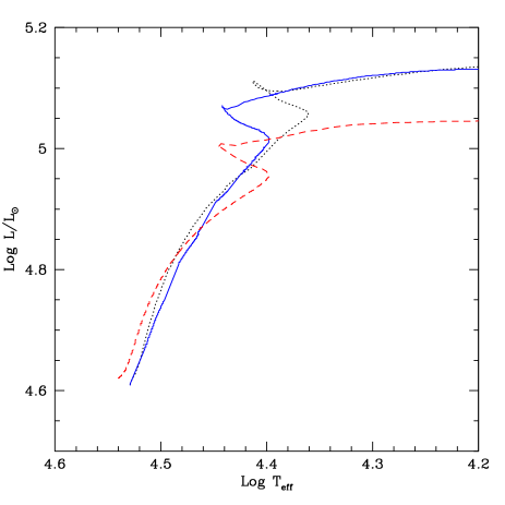
Figure 4: The HR diagram for the MS phase of 3 models of 20 M_⊙ at $Z=0.02$. The broken line (lower turnoff) is for a non–rotating model. The continuous line is for an initial velocity of 300 km/s with the new $D_{\mathrm{h}}$ given by Eq.(19). The track with a dotted line (higher turnoff) is for the same initial velocity with the old $D_{\mathrm{h}}$ given by Eq.(1).

Fig. 4 illustrates the tracks in the HR diagram. We see that the model with the new (and large) $D_{\mathrm{h}}$ has a turnoff inbetween that of the model without rotation and that of the rotating model with the old coefficient $D_{\mathrm{h}}$ given by Eq.(1). This is quite in agreement with the H–profiles and the values of the mass fractions of the convective cores, which are 6.8, 7.1 and 7.7 M${\odot}$ when $X_{\mathrm{c}}=0.33$ for the model with zero rotation, for the model with rotation, with the new and the old $D_{\mathrm{h}}$ respectively. As well known, larger cores make MS tracks extend to higher luminosities. We notice however that the intermediate track with the new $D_{\mathrm{h}}$ is slightly bluer than an average of the other two tracks would suggest. This is due to the larger enrichments of the outer layers in helium, which reduces the opacity and makes the star slightly bluer and brighter.

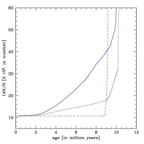
Figure 5: Evolution as a function of time of the abundance ratios $N/H$ at the stellar surface of the 3 models with 20 M_⊙ considered. The meaning of the lines is the same as in Fig. 3 and 4. The continuous (higher) line is that of the rotating model with the new $D_{\mathrm{h}}$.

Fig. 5 completes this picture by showing the evolution with time of the ratio $N/H$ of the nitrogen to hydrogen ratios at the stellar surface. We see that the surface enrichment in nitrogen of the model with the new $D_{\mathrm{h}}$ given by Eq.(19) is larger than the one obtained with old $D_{\mathrm{h}}$ given by Eq.(1). This is quite consistent with what we have just seen above in Fig. 3. The larger $D_{\mathrm{h}}$ makes $D_{\mathrm{shear}}$ larger in the outer layers and the transport of the new helium and nitrogen to the surface is more important. This observational consequence is particularly interesting in view of the new results by Heap (heap (2002)), who has shown very high $N/H$ enrichments in OB stars up to about 50. Future detailed comparisons considering carefully the mass, velocities and abundances of OB stars are necessary to examine whether the models with the new $D_{\mathrm{shear}}$ are better supported by the observations.

5 Conclusions

The following conclusions have been obtained here:

– By expressing the balance between the energy dissipated by the horizontal turbulence and the excess of energy present in the differential rotation on an equipotential which can be dissipated in a dynamical time, we have found a new expression for the coefficient of diffusion $D_{\mathrm{h}}$ by the horizontal turbulence in rotating stars. This new coefficient is typically larger by a factor $10^{2}$ than the one proposed by Zahn (Zahn92 (1992)).
–The differential rotation on an equipotential is found much smaller so that the hypothesis of shellular rotation by Zahn (Zahn92 (1992)) is reinforced.
–A higher horizontal turbulence reduces the importance of the $\mu$–currents and also to a smaller extent the driving of the meridional circulation.
–Numerical models show in agreement with a physical discussion that due to the different effects of the horizontal turbulence on the shears and on the transport of chemicals by circulation, a larger $D_{\mathrm{h}}$ tends to contain the size of the core and at the same time to favour the spread of the processed elements up to the stellar surface.
–The tracks in the HR diagram obtained with the new and larger $D_{\mathrm{h}}$ for rotating stars are in agreement with the above effects.

It will be interesting to further explore the consequences of the larger $D_{\mathrm{h}}$ suggested here for other stellar masses and evolutionary stages.

- (1) Brüggen M. & Hillebrandt W. 2001, MNRAS 320, 73
- (2) Chaboyer B. & Zahn J.P. 1992, A&A 253, 173
- (3) Chaboyer B., Demarque P. & Pinsonneault M.H. 1995a, ApJ 441, 865
- (4) Chaboyer B., Demarque P. & Pinsonneault M.H. 1995b, ApJ 441, 876
- (5) Endal A.S. & Sofia S. 1976, ApJ 210, 184
- (6) Heap S. 2002, in “CNO Elements in the Universe”, Eds. C. Charbonnel, D. Schaerer & G. Meynet, PASP in press
- (7) Heger A., Langer N. & Woosley S.E. 2000, Ap.J. 528, 368
- (8) Heger A.& Langer N. 2000, Ap.J. 544, 1016
- (9) Kippenhahn R.& Thomas H.C. 1970, in Stellar Rotation, IAU Coll. 4, Ed. A. Slettebak, p.20
- (10) Kippenhahn R. & Weigert, A. 1990,“Stellar Structure and Evolution”. Springer Verlag, p. 437
- (11) Maeder A. 1997, A&A, 321, 134 (paper II)
- (12) Maeder A. & Meynet, G. 2000, A&A, 361, 159 (paper VI)
- (13) Maeder A. & Meynet, G. 2001, A&A, 373, 555, (paper VII)
- (14) Maeder A. & Zahn J.P. 1998, A&A, 334, 1000, (paper III)
- (15) Maeder, A., Grebel, E. & Mermilliod, J.C. 1999, A&A 346, 459
- (16) Mestel, L. 1953, MNRAS 113, 716
- (17) Mestel, L. 1965, in “Stellar Structure”, REd. L.H. Aller and D.B. MCLaughlin, Univ. of Chicago press, P.465.
- (18) Meynet G. & Maeder A. 1997, A&A 321, 465 (paper I)
- (19) Meynet G. & Maeder A. 2000, A&A, 361, 101, (paper V)
- (20) Meynet G. & Maeder A. 2001, A&A, 381, L25
- (21) Öpik E.J. 1951, MNRAS 111,278
- (22) Palacios, A., Talon, S., Charbonnel, C. & Forestini, M. 2002, A&A, in press
- (23) Spiegel E. & Zahn J.P. 1992, A&A 265, 106
- (24) Spruit H.C. 2002, A&A 381, 923
- (25) Theado, S. & Vauclair, S. 2001, A&A 375, 70
- (26) Zahn J.P. 1992, A&A 265,115