Blue Straggler Stars: a direct comparison of Star counts and population ratios in six Galactic Globular Clusters

Abstract

The central regions of six Galactic Globular Clusters (GGCs) (M3, M80, M10, M13, M92 and NGC 288) have been imaged using HST-WFPC2 and the ultraviolet (UV) filters (F255W, F336W). The selected sample covers a large range in both central density ($\log\rho_{0}$) and metallicity (${\rm[Fe/H]}$). In this paper, we present a direct cluster-to-cluster comparison of the Blue Stragglers Stars (BSS) population as selected from $(m_{255},m_{255}-m_{336})$ Color Magnitude Diagrams (CMDs). We have found: (a) BSS in three of the clusters (M3, M80, M92) are much more concentrated toward the center of the cluster than the red giants; because of the smaller BSS samples for the other clusters we can only note that the BSS radial distributions are consistent with central concentration; (b) the specific frequency of BSS varies greatly from cluster to cluster. The most interesting result is that the two clusters with largest BSS specific frequency are at the central density extremes of our sample: NGC 288 (lowest central density) and M80 (highest). This evidence together with the comparison with theoretical collisional models suggests that both stellar interactions in high density cluster cores and at least one other alternate channel operating low density GGCs play an important role in the production of BSS. We also note a possible connection between HB morphology and blue straggler luminosity functions in these six clusters.

1 Introduction

Stellar collisions are thought to be the dominant channels for the formation and evolution of various types of unusual stellar objects and binary systems in the dense stellar environments, such as the central regions of Galactic Globular Clusters (GGCs). Among the possible collisionally induced populations, Blue Stragglers Stars (BSS) are surely the most studied. BSS were first discovered by Sandage (1953) in M3. In recent years the realization that BSS are the ideal diagnostic for a quantitative evaluation of the effects of dynamical interactions inside star clusters has led to a remarkable burst of activity in the search for and the systematic study of BSS in clusters. In addition, the Hubble Space Telescope (HST), with its high angular resolution and UV imaging capabilities, has made it possible to search for candidates BSS in the cores of highly concentrated GGCs.

Within this framework we are performing an extensive HST-UV survey in the cores of a selected sample of GGCs searching for various products of binary evolution. In particular, we are constructing an homogeneous database of BSS in the UV-bands. Some results have been already published in a series of papers presenting the BSS content in individual clusters (see Ferraro et al. 1997a, 1999a, 2001 and Paltrinieri et al. 1998, Bellazzini et al. 2002, Ferraro, Paltrinieri & Cacciari, 1999, for a review). In this series of papers we empirically demonstrated that UV-CMDs are the most appropriate planes for the study of BSS.

In this paper, we present a direct comparison of the BSS content in six intermediate to high density ($\log\rho_{0}\sim 2$–5.4) GGCs with intermediate to low metallicity: M13 (NGC 6205), M10 (NGC 6254), M80 (NGC 6093), M3 (NGC 5272), M92(NGC 6341) and NGC 288. In §3 we present the BSS samples discovered in each cluster on the basis of the UV-CMDs, and we discuss the properties and the radial distributions of BSS with respect to normal cluster stars. In §4 we present the comparison of the BSS distribution in the UV-CMDs with that expected from theoretical collisional models.

2 Observations and data analysis

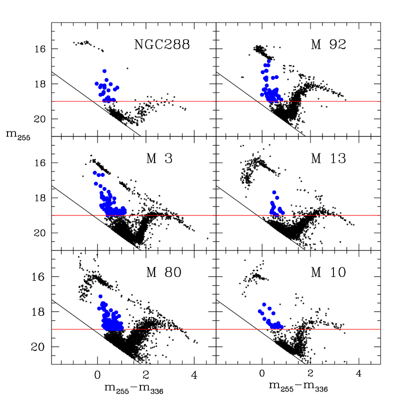
Figure 1: ($m_{255},m_{255}-m_{336}$) CMDs for the selected clusters. Horizontal and vertical shifts have been applied to all CMDs in order to match the main sequences of M3. The horizontal solid line corresponds to $m_{255}=19$ in M3. The bright BSS candidates are marked as large empty circles.

The data-set used in this work consist of a series of HST-WFPC2 exposures covering the central regions of six GGCs: M3, M10, M13, M80, M92 and NGC 288. In Table 1 we summarized the main characteristics of each cluster: metallicity (${\rm[Fe/H]}$) from Zinn & West (1984), central density ($\rho_{0}$ and mass (from Trager & Meylan 1993), distance ($d$) (from Ferraro et al. 1999b), and central dispersion velocity ($\sigma_{0}$) (from Trager & Meylan 1993). For each cluster, the Planetary Camera (PC) was roughly centered on the cluster center (in the case of NGC 288 the cluster center was outside the field of view of the PC - see Figure 1 by Bellazzini et al. 2002). By adopting this observational strategy a significant fraction of the cluster luminosity has been sampled with a single HST pointing, In Table 3 (column 2) the fraction of the cluster luminosity sampled ($L_{S}/L_{T}$) in each cluster is reported. Here we present the results obtained using the mid-UV (F255W) and near-UV (F336W) filters, those best suited for picking out BSS. Table 2 lists the total duration of the exposures in each filter for the six clusters.

All the photometric reductions (with the exception of NGC 288; see Bellazzini et al. 2002) have been carried out using ROMAFOT (Buonanno et al. 1983), a package specifically developed to perform accurate photometry in crowded fields. The standard procedure described in Ferraro et al. (1997a) was adopted. More details on the reduction procedure and the entire dataset secured in these clusters can be found in some specific papers already published (see for example Ferraro et al. 1997a for M3 and Ferraro et al. 1999a for M80). Briefly, the images in the same filter were aligned and combined in order to obtain a median image in each filter. We used the combined F255W image as reference frame for searching the objects in each field. Then the PSF fitting procedure was separately performed on each individual frame, and an average magnitude was computed for each star. The instrumental magnitudes were finally transformed into the STMAG system, using Table 9 of Holtzmann et al. (1995).

3 Results

In the UV cluster light is dominated by hot stars, specifically the blue HB stars and the BSS. (see for example Figure 1 by Ferraro, Paltrinieri & Cacciari 1999). Since the BSS are one of the hottest sub-populations in the cluster, they are easily separated from the cooler Turn-Off and SGB stars. Indeed, in previous papers (Ferraro et al. 1997a, 1999a, 2001 and Paltrinieri et al. 1998, Ferraro, Paltrinieri & Cacciari, 1999) we have shown that UV-CMDs, in particular the $(m_{255},~{}m_{255}-m_{336})$ plane, are ideal for selecting BSS.

Figure 1 shows the ($m_{255},~{}m_{255}-m_{336}$) CMDs for the six clusters. More than 50,000 stars are plotted in the six panels of Figure 1. As can be seen, in this plane, the BSS populations define a clean and well-defined sequence spanning $\sim 3$ mag in $m_{255}$. Further, they are clearly distinguishable from SGB-TO stars. In order to select the BSS samples we followed the same criteria that we adopted for M3. In Ferraro et al. (1997a), the global population of BSS was divided in two sub-samples: (a) bright BSS with $m_{255}<19$ and (b) faint BSS with $19.0<m_{255}<19.4$. To apply the same criteria to the other clusters shown in Figure 1, the CMD of each cluster has been shifted to match that of M3 by using the brightest portion of the HB as the normalization region. Figure 1 shows the UV-CMD after the alignment. Thus, the solid horizontal line (at $m_{255}=19$) in the figure shows the cut-off magnitude for the bBSS sample. In this paper we are comparing the BSS content in clusters with quite different structural parameters. The level of difficulty in the detecting and the measuring of (especially faint) BSS varies from cluster to cluster. Thus, we decided to compare the samples by using only the bright BSS samples (hereafter bBSS). The number of bright BSS ($N_{bBSS}$) identified in each cluster is listed in Table 3.

3.1 bBSS radial distribution

As pointed out by many authors most BSS in GGCs are found to be centrally concentrated with respect to normal stars. Since the central relaxation time in these systems is much less than the cluster age, this result is generally ascribed to dynamical mass segregation and can be interpreted as an evidence that BSS are more massive than the comparison stars.

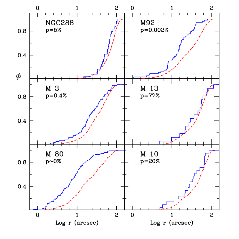
Figure 2: Cumulative radial distributions for the bright BSS (solid line) with respect to the RGB stars (dashed line) as a function of their projected distance ($r$) from the cluster center for each of the six clusters. The probability that the two populations are extracted from the same distribution is also reported in each panel.

We have determined the radial distributions of the bBSS of the six GGCs using the RGB stars (from the tip down to the SGB ) as a “reference” population. The RGB stars have been selected in the $(m_{555},m_{336}-m_{555})$ CMD, i.e. roughly a $(V,~{}U-V)$ CMD in order to reduce any bias which might be introduced by the poor photometry for the very red stars in the UV bands. The cumulative radial distributions for the bBSS and the RGB stars are plotted in Figure 2 as a function of the projected distance ($r$) from the cluster center. It is evident from the plots that the BSS (solid line) are significantly more centrally concentrated than RGB stars (dotted line) in M3, M92 and M80. A Kolmogorov-Smirnov test has been applied to the two distributions, in each cluster, to check the statistical significance of the detected differences. The test yields the probability that the bBSS population and the RGB stars are extracted from the same parent distribution. The probability values obtained in each cluster are reported in Figure 2. The effect is strongly statistically significant in the case of M3, M92 and M80. For NGC 288 and M10 the BSS are more concentrated that the RGB but the results are significant at only roughly the $2\sigma$ and $1\sigma$ levels respectively.

At first glance the radial distribution of the BSS in M13 appears to be indistinguishable from the other cluster stars. Since it is difficult to imagine any BSS formation scenario in which the BSS are not at least somewhat centrally condensed, we have more carefully examined the role of the small M13 bBSS sample. A series of Monte Carlo simulations have been performed in which $10^{3}$ subsamples of the same number of the bBSS population found in M13 (16) have been randomly extracted from the M3 bBSS population (72). Then, the radial distribution of each subsample was compared with that of the RGB stars of M3. A KS test has been applied to quantify the significance of the differences. In these simulations drawn from a sample in which the central concentration of the BSS has been convinvingly shown, 40% of the M13-like samples have $p>20\%$ that the BSS and RGB have the same distribution. Less than 10% have as a convincing a case for different distributions as in M3. About $6\%$ of the M13-like samples have $p$ as large as for the true M13 comparison. In another test, two M13 BSS were arbitrary moved from the middle of the distribution to the inner part and $p$ dropped from 0.77 to 0.34. We conclude that the M13 bBSS sample is too small to make a definitive statement about its central concentration. Our M13 results are consistent with no central concentration, but they are not inconsistent with a central concentration even as large as that of M3.

The case of NGC 288 deserves a short comment since the location of the center in this cluster is quite uncertain. The radial distribution plotted above could be affected by large uncertanties. In accordance with Bellazzini et al. (2002) we adopted the coordinates listed by Webbink (1985), and the cluster center turns out to be located just outside the field-of-view of the PC (see their Figure 1).

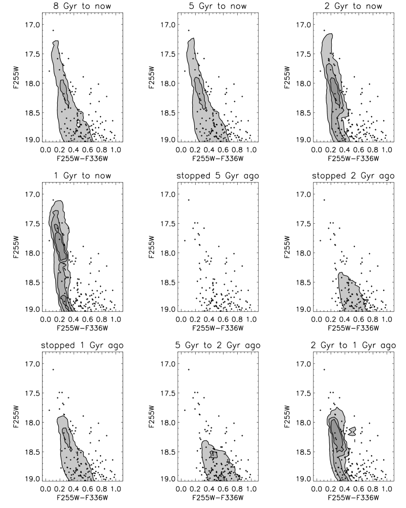
Figure 4: The distribution of bright blue stragglers in the color-magnitude diagram for M80, compared to theoretical distributions. The observations are plotted as crosses, and the greyscale contours give the theoretical distributions, with darker colors indicating more blue stragglers. The different panels correspond to different eras of constant blue straggler formation, as indicated at the top of each panel.

We can make an additional quantitative comparison by using the parameters $r_{1/2}^{\scriptscriptstyle\rm BSS}$ (the radius containing half the bBSS sample) and $f_{\scriptscriptstyle\rm RGB}$(the fraction of the total RGB sample contained within $r_{1/2}^{\scriptscriptstyle\rm BSS}$). Values for $r_{1/2}^{\scriptscriptstyle\rm BSS}$ and $f_{\scriptscriptstyle\rm RGB}$ are listed in Table 3 along with the core radius ($r_{c}$). With the exception of NGC 288 (for which we took the value from Trager, Djorgovski & King, 1993), the $r_{c}$ was independently determined in each cluster by fitting a King model to the observed density profile (see for example Figure 4 in Ferraro et al. 1999a). These values confirm the general impression from Figure 2,that the BSS are much more concentrated than the RGB in M80, M3 and M92. Thus, even considering the brightest part of the BSS distribution in M80, we have fully confirmed the previous results by Ferraro et al. 1999a, who suggested that the BSS in M80 are the most concentrated population observed in a GGCs.

In Figure 3 the magnitude distributions (equivalent to a luminosity function—LF) of bBSS for the six clusters are compared. In doing this we use the parameter $\delta m_{255}$ defined as the magnitude of each bBSS (after the alignment showed in Figure 1) with respect to the magnitude threshold (assumed at $m_{255}=19$ - see Figure 1). Then $\delta m_{255}=m^{bBSS}_{255}-19.0$. From the comparison shown in Figure 3 (panel(a)) the bBSS magnitude distributions for M3 and M92 appear to be quite similar and both significantly different from those obtained in the other clusters. This is essentially because in both these two clusters the bBSS magnitude distribution seems to have a tail extending to brighter magnitudes (the bBSS magnitude tip reaches $\delta m_{255}\sim-2.5$). A KS test applied to these two distributions yields a probability of $93\%$ that they are extracted from the same distribution. In panel(b) we see that the bBSS magnitude distribution of M13, M10 and M80 are essentially indistinguishable from each other and significantly different from M3 and M92. A KS test applied to the three LFs confirms that they are extracted from the same parent distribution. Moreover, a KS test applied to the total LFs obtained by combining the data for the two groups: M3 and M92 (group(a)), and M13, M80 and M10 (group(b)) shows that the the bBSS-LFs of group(a) and group(b) are not compatible (at $3\sigma$ level).

It is interesting to note that the clusters grouped on the basis of bBSS-LFs have some similarities in their HB morphology. The three clusters of group(b) have an extended HB blue tail; the two clusters of group(a) have no HB extention. Could there be a connection between the bBSS photometric properties and the HB morphology? This possibility needs to be further investigated.

Finally we note that the magnitude function for the bBSS in NGC 288 (solid line in panel (b)) is significantly different than that of all the other clusters.

3.2 Specific Frequency

In order to properly compare the BSS populations in different clusters, the BSS number must be normalized to account for the size of the total cluster population. For this reason we have defined various specific frequencies. In Ferraro, Fusi Pecci & Bellazzini (1995) we used $S4_{\scriptscriptstyle\rm BSS}$ (the BSS number normalized to the integrated bolometric luminosity of the surveyed region in units of $10^{4}L_{\odot}$). Analogously, in Ferraro et al. (1999a) we defined a more appropriate specific frequency:

$${F_{\scriptscriptstyle\rm HB}^{\scriptscriptstyle\rm BSS}}={{N_{\scriptscriptstyle\rm BSS}}\over{N_{\scriptscriptstyle\rm HB}}}$$

where $N_{\scriptscriptstyle\rm BSS}$ is the number of BSS and $N_{\scriptscriptstyle\rm HB}$ is the number of HB stars in the same area. The two ratios are similar, since in absence of any special segregation of HB stars with respect to the ”normal” cluster-star, the observed number of HB stars $N_{\scriptscriptstyle\rm HB}$ is an excellent indicator of the sampled cluster luminosity. In fact, the simple relation by Renzini & Buzzoni (1986):

$$N_{j}=B(t)L_{S}t_{j}$$

easily links the number of stars sampled in any post main sequence stage ($N_{j}$) with the sampled cluster luminosity ($L_{S}$) and the duration of the phase ($t_{j}$). $B(t)$ is the specific flux of the population. Following Renzini & Buzzoni (1986) we assume $B(t)\sim 2\times 10^{-11}{~{}\rm stars}\,L_{\odot}^{-1}\,{\rm yr}^{-1}$ for an old population of $10^{10}\,{\rm yr}$.

Thus, assuming $t_{\rm HB}\sim 10^{8}\,{\rm yr}$, we can expect to sample $2\times 10^{-3}$ HB stars for each solar luminosity sampled in a given stellar population.

The ${F_{\scriptscriptstyle\rm HB}^{\scriptscriptstyle\rm BSS}}$ ratio has the advantage that it is a purely observative quantity and it can be easily computed in the UV-CMDs since the HB population is quite bright in these planes and the HB sequence is well separated from the other branches. However, while in the following discussion we will mainly use the ${F_{\scriptscriptstyle\rm HB}^{\scriptscriptstyle\rm BSS}}$ ratio, the $S4_{\scriptscriptstyle\rm BSS}$ is also computed for each cluster and the values are listed in Table 3 for sake of comparison.

As discussed in Section 3 we consider only the bright BSS, hence $N_{\scriptscriptstyle\rm bBSS}$ is the number of bright bBSS (according to the original definition by Ferraro et al. (1997a)). The values of $F_{\scriptscriptstyle\rm HB}^{\scriptscriptstyle\rm bBSS}$ are listed in Table 3. As can be seen $F_{\scriptscriptstyle\rm HB}^{\scriptscriptstyle\rm bBSS}$ varies by a factor 13 from M13 to NGC 288. Interesting enough NGC 288, the cluster with the lowest central density, shows the largest bBSS specific frequency. As already noted by Bellazzini et al. (2002) this cluster turns out to have as many bBSS as HB stars over the sampled area. Though the number of bBSS detected in the cluster is intrinsically small ($\sim 30$) the result is surprising: $F_{\scriptscriptstyle\rm HB}^{\scriptscriptstyle\rm bBSS}$ is comparable with what found in the central region of the core-collapsing cluster M80 by Ferraro et al. (1999a). If we consider only the PC field of view, the $F_{\scriptscriptstyle\rm HB}^{\scriptscriptstyle\rm bBSS}$ in M80 rises up to 0.7.

The central density of a cluster is not the only factor which determines the number of collision products we expect to see. Collisions involving binary star systems are more likely than collisions between single stars and have a significant probability of producing a stellar merger. We used equation 14 from Leonard (1989) in order to estimate the number of binary-binary (bb) encounters occuring per Gyr ($N_{bb}$) in the core of each cluster listed in Table 1. Adopting the distance modulus listed in Table 1, the $r_{c}$ listed in Table 3, $\sigma_{0}$ and the central density $Log(\rho_{0})$ listed in Table 1 (from Pryor & Meylan (1993)), assuming an average mass of 0.2$M_{\odot}$ (Kroupa 2001), we computed $t_{bb}$ (the mean interval between collisions) from equation (14) by Leonard (1989) and derived the expected number of encounters, per Gyr, as a function of the binary fraction ($f_{b}$) in the core.

In doing this, the semimajor axis which separates hard from soft binaries ($a_{hs}$) has been computed for each cluster according to the following relation:

$$a_{hs}={{GM}\over{9\sigma_{0}^{2}}}$$

derived by combining equation 4 of Leonard & Linnell (1992) with the Kepler’s third law. The semimajor axes computed for each cluster and expressed in AU are listed in Table 4.

Following Leonard (1989) we multiplied $t_{bb}$ by a factor of two in order to take into account the fact that not all encounters lead to a physical collision. The rate of single-binary collisions can also be estimated from Leonard’s results. In his equation 8 if one assumes that the pericenter distance is proportional to binary semimajor axis, like in binary-binary collisions, and that $M_{1}=M_{\star}$, $M_{2}(binary)=1.5\,M_{\star}$, one finds a factor of 5 instead of his 6 in the cross section. Thus the number of single-binary encounters is roughly the 5/6 the number of binary-binary encounters.

In Table 4 we list the results with three different $f_{b}$ values, respectively 0.2 and 1.00. These values should be considered as indications of the effectiveness of physical collisions in the cluster cores. It is clear that the bb (or sb) collision channel is more than one order of magnitude more efficient in a dense cluster like M80 than in a low density cluster like NGC 288. Therefore, the high specific frequency of blue stragglers in NGC 288 suggests that the binary fraction in NGC 288 is much higher than the binary fraction in M80. Only then would one expect a similar encounter frequency in the two clusters. Note that a cluster like M80 may have originally had a higher binary fraction but because of the efficiency of encounters, those primordial binaries were “used up” early in the history of the cluster, producing some collisional BSS which have evolved away from the MS (see for example the evolved E-BSS population found in M3 and M80 by Ferraro 1997a, 1999a).

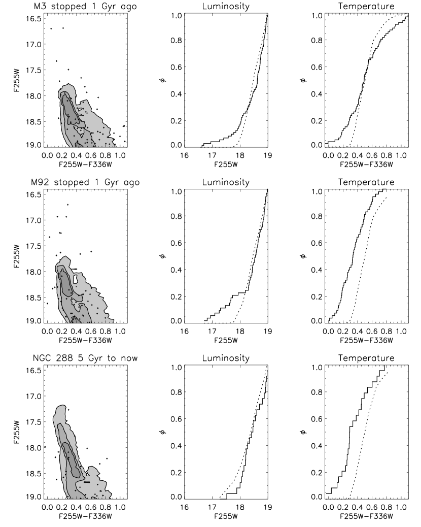
Figure 8: Same as figure 7, for M3, M92 and NGC 288. M3 and M92 contain the brightest blue stragglers in our sample, and so the best-fit theoretical distribution is one in which young blue stragglers (up to 1 Gyr old) are found. However, because of the spread in temperature, these clusters are best fit by a truncated blue straggler formation model, like M80, M10 and M13. NGC 288 is different from the previous 5 clusters—its blue straggler distribution is extremely well fit by a model which has had essentially constant blue straggler formation over the lifetime of the cluster right to the present day.

We should note that on the basis of the simulation results shown in Figure 8 and in Table 4 the binary-binary channel can still account for the number of the BSS observed in NGC288 if a large enough percentage of binary fraction is assumed to reside in the core.

However, without invoking ad hoc binary content, a more natural explanation for the origin of BSS in NGC 288 (as discussed in Bellazzini et al. (2002)) is the mass transfer process in primordial binary systems (Carney et al 2001). Here we probably have another confirmation of the scenario suggested by Fusi Pecci et al. (1992, and references therein): BSS living in different environments have different origins.

4 Collisional Models

From our sample of six clusters with rather diverse bBSS populations we can select pairs with similarities in parameters like density, metallicity, velocity dispersion, or we can search for trends in bBSS populations as some parameter varies. There are two quite striking and unsuspected results. First, the two clusters at the high and low density extremes, M80 and NGC 288, have the largest bBSS specific frequencies. Second, two clusters which are in most ways quite similar, M3 and M13, have very different bBSS populations.

To aid our understanding of the BSS populations in these clusters, we present a comparison of the photometric characteristics of the BSS observed in the selected clusters with some collisional models. The models we used in this paper are described in detail in Sills & Bailyn (1999), and have been applied to 47 Tucanae (Sills et al. 2000). We assume that the blue stragglers in the central regions of the six clusters are all formed through stellar collisions between single stars during an encounter between a single star and a binary system. While binary-binary collisions may well be important, we do not currently have the capability of modeling the BSS they might produce. The trajectories of the stars during the collision are modeled using the STARLAB software package (McMillan & Hut 1996). The masses of the stars involved are chosen randomly from a mass function for the current cluster and a different mass function which governs the mass distribution within the binary system. A binary fraction, and a distribution of semi-major axes must also be assumed. The output of these simulations is the probability that a collision between stars of specific masses will occur. We have chosen standard values for the mass functions ($dN(M)\propto m^{-(1+x)}dM$) and binary distribution. The current mass function has an index $x=-2$, and the mass distribution within the binary systems are drawn from a Salpeter mass function ($x=1.35$). We chose a binary fraction of 20% and a binary period distribution which is flat in $\log P$. The total stellar density was taken from the central density of each cluster. The effect of changing these values is explored in Sills & Bailyn (1999). The collision products are modeled by entropy ordering of gas from colliding stars (Sills & Lombardi 1997) and evolved from these initial conditions using the Yale stellar evolution code YREC (Guenther et al. 1992). The models reported here used a metallicity of ${\rm[Fe/H]}=-1.6$, which is approximately correct for 4 of the clusters investigated in this paper. BSS populations should not be strongly dependent on metallicity. By weighting the resulting evolutionary tracks by the probability that the specific collision will occur, we obtain a predicted distribution of BSS in the color-magnitude diagram.

In order to explore the effects of non-constant BSS formation rates, we considered a series of truncated rates. In these models we assumed that the BSS formation rate was constant for some portion of the cluster lifetime, and zero otherwise. This assumption is obviously unphysical—the relevant encounter rates would presumably change smoothly on timescales comparable to the relaxation time. However these models do demonstrate how the distribution of BSS in the color-magnitude diagram depends on when the BSS were created, and thus provide a basis for understanding more complicated and realistic formation rates.

4.1 Comparisons with data

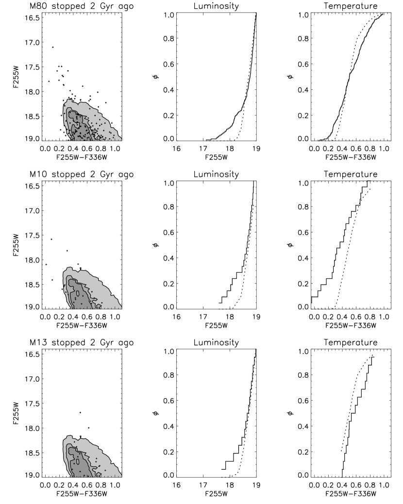
Figure 7: The observed blue stragglers (crosses in the CMD, solid lines in the luminosity and temperature functions) and the best fit theoretical distribution, as determined from KS tests on the luminosity and temperature functions. This figure shows the results for M80, M10 and M13. In all cases, the nominal best-fit distribution is one in which the blue stragglers stopped forming 2 Gyr ago. However, only for M13 is this actually plausible. M80, and to a lesser extent M10 were forming blue stragglers more recently than 2 Gyr ago, since we see a population of BSS brighter than $m_{255}=18$. On the other hand, the temperature function (i.e. the distribution of BSS in evolutionary state) is very well fit by this truncated distribution.

Some comparisons between the models and the HST observations are shown in figures 4–8. In figures 4, 5 and 6, we compare our theoretical predictions to the BSS population of M80. The theoretical predictions have been normalized by the total number of predicted blue stragglers for each cluster; this allows us to more easily compare the shapes of the distributions. Figure 4 is an example of the predicted distribution of BSS in the $m_{255},~{}m_{255}-m_{336}$ color-magnitude diagram for M80. The theoretical predictions are shown as greyscale contours, with the darker colors indicating more BSS in that region of the CMD. The observed blue stragglers are shown as crosses. Each of the panels is a different assumption for the BSS formation rate, as indicated on the top of the panel. The differences between the models can be understood in terms of lifetimes of the individual collision products which make up the distributions. For example, if BSS production stopped 5 Gyr ago (center panel), we predict that there should be no observed bBSS at present because all the massive BSS would have had time to evolve off to the giant branch. At the other extreme, if all the BSS were formed in the last Gyr (panel marked “1 Gyr to now”), only a few of the very brightest (i.e. most massive) would have even started moving towards the subgiant branch. It is worth pointing out that the brightest BSS shown in these predictions are not on the standard zero age main sequence, but begin their lives to the red. These are stars which were formed from the merger of two fairly evolved main sequence stars, and so they do not have enough hydrogen fuel left at their cores after the merger to return to the ZAMS (Sills et al. 1997).

Figure 5 gives the luminosity function for each of the model distributions for M80. The data are shown as the solid line, while the dotted line is the theoretical prediction for the formation times shown on the top of each panel. The luminosity functions are good probes of the mass distribution of blue stragglers, since the correlation between mass and luminosity is quite tight. The luminosity functions show, as do the CMD distributions, that bright BSS require recent formation. They also show that the relative numbers of brighter and fainter bBSS is not correct in our models. If we model the fainter bBSS very well (as in the panel marked “stopped 2 Gyr ago”), then our models under-predict the number of blue stragglers between $m_{255}=17$ and 18.

Figure 6 gives the equivalent “temperature function” for M80. This is the cumulative number of stars in each color (i.e. temperature) bin, in direct analogy to the luminosity function. The distribution of blue stragglers in color can be used to study the age or age spread of the BSS. Evolutionary tracks for stars of these masses are confined to a fairly narrow range in luminosity between the main sequence and the base of the giant branch, so the luminosity function does not give the entire picture. The temperature function is useful for distinguishing between populations which have lots of main sequence stars and populations with many subgiants. As in figure 5, the data are shown as the solid line, while the dotted line is the theoretical prediction for the formation times shown on the top of each box.

We performed KS tests on the luminosity and temperature functions for each cluster and each theoretical distribution. Figures 7 and 8 gives the best fit model distribution for each cluster, its luminosity function, and its temperature function. We will comment on each cluster individually here, and then draw some general conclusions in the next section.

M80: The fainter bBSS are very well fit by a distribution in which formation was truncated about 2 Gyr ago. However, there is a significant population of BSS which extends up to 2.5 magnitudes above the turnoff, which is not predicted by such a model and which suggests that some BSS formation continues until the present. Ferraro et al. (1999a) suggested that the large BSS population in M80 is due to the stellar interactions which are delaying the core collapse process. Now we add the evidence that many of these BSS are relatively old ($t>2$ Gyr). These results together suggest that the process of holding off the core collapse can be rather extended.

M10: The BSS in this cluster are fit by different formation models in the temperature and luminosity planes. However, the difference between the KS probability for the best fit to luminosity function (BSS formation ended 2 Gyr ago) and the best fit for temperature function (BSS formation ended 1 Gyr ago) is small. The luminosity function has a 16% probability of being drawn from the first distribution, and a 10% probability of being drawn from the second distribution.

M13: Of all the clusters in this paper, this one is the most believable for showing a truncated BSS distribution. There is no evidence for very bright BSSs close to the main sequence. The only BSS brighter than $\delta m_{255}=2.5$ is very red, consistent with an evolved object.

M3: None of the collisional models fit this cluster very well. The best fit for the luminosity function, as shown in figure 8, is a model in which the BSS stopped forming about 1 Gyr ago (3% KS probability). However, the temperature function for the same model has almost zero probability of being drawn from the same distribution as the data, and the best fit temperature function is the scenario in which the BSS stopped forming 2 Gyr ago. In all cases, including the models which predict BSS formation right up to the present day, we under-predict the number of very bright blue stragglers.

M92: The best fit to both the luminosity and temperature functions is a model in which the BSS formation was truncated 1 Gyr ago. However, there are also very bright blue stragglers in this cluster, suggesting that blue straggler formation has continued to the present day or that the blue stragglers produced in this cluster are not well modeled by collisions between two stars.

NGC 288: This cluster is significantly different from the previous 5, in that we do not expect that the BSS formed in this cluster are the products of stellar collisions. The density is simply too low. We also know that the binary fraction in the core is measured to be $\sim 10$ to 38% (Bellazzini et al. 2002), so BSS formed in this low density cluster should be the result of binary evolution rather than stellar collisions. By assuming that binary merger BSS are similar to collisional BSS we can still expore the BSS formation history in NGC 288. The best fit distribution for this cluster, at the 65% level, is achieved when the BSS were formed at a constant rate over the entire lifetime of the cluster, right up to the present day. This result is significantly different from the other five clusters investigated in this paper. Perhaps, it could be an indication of the different formation histories of binary mergers and collisions. It is also possible that the difference between this cluster and the other 5 could be a result of different evolutionary tracks for binary merger and collision products.

4.2 Indications and Trends

The first conclusion that we draw from the models is that since we are limiting our study to BSS brighter than the limit of $m_{255}=19.0$, we have no information about BSS formation earlier than about 5 Gyr ago. On the other hand, we can state with certainty that BSS have been formed in all these clusters during the last 5 Gyr. In all clusters, this formation is not confined to the very recent past; rather, it has lasted over the entire time that we can probe, and in fact seems to be concentrated at earlier epochs.

The KS tests on the luminosity and temperature functions give the best results for distributions in which BSS stopped forming 1–2 Gyr ago in all clusters except NGC 288. These “best” fits are clearly not good fits, however. In most of the clusters, there is a population of bright BSS that was formed more recently. Our models consistently under-predict the number of bright BSS compared to the number of fainter, redder BSS. There are a number of possible reasons.

The first, and most likely, discrepancy is in the formation rate of blue stragglers. We have assumed a constant formation rate over the some times, and zero otherwise. If, instead, blue stragglers were formed at some (more or less) constant rate between 5 and 2 Gyr ago, and then experienced a reduced (but not zero) blue straggler formation rate to the present day, the predicted distribution would match the observations better. It is very unlikely that the blue straggler formation rate changes sharply between zero and a constant value. Rather, the formation rate is going to be smoother function of central density, velocity dispersion, single star mass function and the number and nature of binary systems in the cluster. The simple models used in this paper should be taken as indications of formation eras only.

It is also possible that the stellar evolutionary models which go into these blue straggler distributions are not accurate. If we were overestimating the lifetimes of the faint blue stragglers or underestimating the lifetimes of the bright blue stragglers, we would see this kind of mismatch between observations and data. It is difficult to understand how the evolutionary tracks would be overestimating the lifetimes of the faint blue stragglers. The lower the mass of the collision product, in general, the more similar it is to a normal star of the same mass, and so its evolutionary track is very much like normal stars—something we understand quite well. In order to underestimate the lifetimes of the brighter blue stragglers, the collision products would have to mix more hydrogen into their cores than is currently predicted. Rapid rotation is a plausible mechanism for this mixing, although we would have to have some process by which the lower mass BSS were not rotating as rapidly. It is also possible that the bright blue stragglers could actually be the merger of three stars rather than two (as is expected to happen in binary-mediated collisions), and so our evolutionary models will not be applicable. The merger product of three $0.4\,M_{\odot}$ stars will have a higher percentage of hydrogen in its core than the product of two $0.6\,M_{\odot}$ stars, but approximately the same mass.

The difference between M3 and M92 on one hand, and M10, M13 and M80 on the other is primarily the existence of a few very bright blue stragglers in the first group of clusters. In all 5 clusters, the blue stragglers fainter than about $m_{255}=18.5$ are very well modeled by the same distribution (a truncated formation scenario, suggesting that blue straggler formation rates should be weighted towards 3–5 Gyr ago). The fact that M3 and M92 are better fit by a formation scenario in which BSS formation ended more recently is simply a reflection of the number of very bright BSS in these clusters. These bright blue stragglers could be an indication of continued BSS formation, or of a different binary distribution (which produced more triple collisions). M3 does have a significant population of BSS in the outer part of the cluster which are thought to be the result of binary mergers (Ferraro et al. 1997a). This fact does set M3 apart from M13, M10, & M80, which have few exterior BSS. Unfortunately M92 also has few exterior BSS so they cannot be invoked to explain the M3/M92 similarity.

As noted in Section 3.1, another very interesting point is that M10, M13 and M80 (which share a common BSS Luminosity function) all have blue tail components to their horizontal branches, while M3, M92 and NGC 288 do not. M3 and M13 are also a classic second-parameter pair (see Ferraro et al. 1997c), referring to the difference in their horizontal branch morphology without an obvious difference in any other cluster parameter: they have the same metallicity, central density, total mass, and very similar velocity dispersions. (The two clusters may have slightly different ages, which may or may not affect horizontal branch morphology—see Rey et al. 2001, Davidge & Courteau 1999, Ferraro et al. 1997c). From these data, there is certainly a suggestion that BSS population could be connected to the second parameter. From the comparisons in this paper, it seems that it is not the total number of BSS or their specific frequency, but rather the kind of BSS which are produced in “blue tail” clusters which is different from those produced in non-blue tail clusters. If this link between BSS and horizontal branch morphology is real, then it suggests that the second parameter could be related to either stellar collisions and encounters, or to binary evolution.

5 Conclusions

In this paper, we have compared the blue straggler distribution in six galactic globular clusters: M3, M10, M13, M80, M92 and NGC 288. The blue stragglers were observed in the HST UV filters F255W and F336W. The clusters have similar total masses, and velocity dispersions; have intermediate to low metallicities and span a range in central density. We studied the properties of the blue stragglers relative to other cluster populations; and we compared the observed blue straggler distributions with theoretical models of collision products in globular clusters.

Whether they formed via a collisional channel or a merged primoridial binary channel, BSS are the most massive stars in GGCs other than neutron stars or possibly some white dwarfs. Since dynamical relaxation times are typically shorter than BSS lifetimes they should settle toward the cluster center. BSS formed from merged primordial binaries have the entire cluster lifetime to settle. Collisions occur most often in high density regions and most often involve binaries providing yet another reason to expect BSS to be found near cluster centers. Indeed, it is difficult to image a BSS formation scenario which would not lead to a centrally condensed BSS distribution. Our results are consistent with this expectation: M3, M92, & M80 show strong central concentrations; the BSS in M10 and NGC 288 are most likely centrally condensed; while the BSS in M13 could have the same distribution as the RGB, they could also have a central concentration similar to that of M3. The small sample size is not adequate to definitively determine the radial distribution.

The specific frequency of blue stragglers compared to the number of horizontal branch stars varies from 0.07 to 0.92 for these six clusters, and does not seem to be correlated with central density, total mass, velocity dispersion, or any other obvious cluster property. We do not have measurements of the binary fraction in most of these clusters. Binary stars impact the blue straggler populations in a number of ways. BSS can be formed from binary evolution in any environment, although binary systems in dense environments will be different from those in sparse environments—close binaries will be hardened by encounters (increasing the number of “binary merger” BSS), but wide binaries are also disrupted (decreasing the number of “binary merger” BSS). The relative rates of these events is an important factor in looking at blue stragglers in clusters. Binary systems also facilitate close interactions between stars because they have a large cross section compared to single stars, so we expect that clusters with a large binary fraction to have both more collisional and binary merger blue stragglers.

Fusi Pecci et al. (1992, and references therein) presented a qualitative interpretative scenario concerning the possible origin of BSS in GGCs. They suggest that BSS in loose clusters might be produced from coalescence of primordial binaries. In high density GGCs (depending on survival-destruction rate of primordial binaries) BSS might mostly arise from stellar interactions, particularly those which involve binaries (Ferraro, Fusi Pecci & Bellazzini, 1995). In this scenario one could find clusters where more than one mechanism is at work in generating BSS. In fact Ferraro et al. (1993, 1997a) found that the radial distribution and the luminosity functions of BSS in the center of M3 are consistent with a collisional origin, while in the outer regions they are consistent with a primordial binary origin. The paucity of BSS in M13 suggests that either the primordial population of binaries in M13 was poor or that most of them were destroyed. Alternatively, as suggested by Ferraro et al. (1997b), the mechanism producing BSS in the central region of M3 is more efficient than M13 because M3 and M13 are in different dynamical evolutionary phases.

The evidence shown above suggests that different channels of BSS formation should be at work and/or a large difference in the binary fraction should be present in NGC 288 in order to produce such a large BSS frequency in a cluster with such different structural parameters. Bellazzini et al. (2002) measured the binary fraction in the core of NGC 288 to be between 10% and 38%. Similar measurements for M3, M13, and M80 will be extremely helpful in solving this mystery.

According to simple models, BSS formation occured in all clusters over last 5 Gyr at least, and more were formed 2–5 Gyr ago than in the recent past. This result needs to be tested using models of globular cluster evolution in which the feedback between stellar collisions and cluster evolution is modeled explicitly. Our assumption of a BSS formation rate which is either constant or zero is unphysical, and more complicated models are clearly required.

Finally, we note the possible connection between horizontal branch morphology and blue straggler population characteristics. Of our six clusters, three have HB blue tails (M10, M13, M80), and three do not. The three with blue tails have the same blue straggler luminosity function, which spans about 1.5 magnitudes compared to 2.5 magnitudes in M3 and M92. This suggests that blue straggler populations and the horizontal branch second parameter may be linked in some way, perhaps through the complicated world of binary systems and their effect on cluster evolution and populations.

Figure 3: Cumulative magnitude distributions for the bright BSS for each of the six clusters. The $\delta m_{255}$ parameter is the difference in magnitude with respect to the limit threashold ($m_{255}=19$) for bright-BSS, see text. In Panel (a) the BSS distributions for M3 and M92 (the two clusters for which the BSS distribution extends up to more than two magnitudes brighter than the threashold) are compared. In Panel (b) the BSS magnitude distributions for the other 4 clusters are plotted.

Figure 5: Luminosity functions for the bright blue stragglers in M80 (solid line), compared to theoretical predictions (dotted line). The different panels correspond to different eras of constant blue straggler formation, as indicated at the top of each panel. The luminosity functions are good probes of the mass function of blue stragglers. This figure shows that the theoretical models do not accurately model the relative numbers of fainter and brighter blue stragglers.

Figure 6: Temperature functions for the bright blue stragglers in M80 (solid line), compared to theoretical predictions (dotted line). The different panels correspond to different eras of constant blue straggler formation, as indicated at the top of each panel. The temperature functions are good probes of the bulk evolutionary state of the population of blue straggler stars, indicating whether the stars are all on the main sequence (as in the panel marked “1 Gyr to now”) or closer to the subgiant & giant branches (as in the panel marked “stopped 2 Gyr ago”). The BSS in M80 show a significant spread in evolutionary state.

Table 1: Cluster parameters

Cluster	$[{\rm Fe/H]}$	$Log\rho_{0}$	$Mass$	$d$	$\sigma_{0}$
		$[M_{\odot}\,pc^{-3}]$	$[Log(M/M_{\odot})]$	$[{\rm kpc}]$	$[{\rm km\,s^{-1}}]$
NGC 5272(M3)	$-1.66$	3.5	5.8	10.1	5.6
NGC 6205(M13)	$-1.65$	3.4	5.8	7.7	7.1
NGC 6093(M80)	$-1.64$	5.4	6.0	9.8	12.4
NGC 6254(M10)	$-1.60$	3.8	5.4	4.7	5.6
NGC 288	$-1.40$	2.1	4.9	8.8	2.9
NGC6341 (M92)	$-2.24$	4.4	5.3	9.0	5.9

Table 2: WFPC2 exposure times

Cluster	F336W-Exp [s]	F255W-Exp [s]
M3	3340	1200
M13	560	200
M80	2400	1160
M10	1500	5200
NGC 288	3760	700
M92	3800	2200

Table 3: Bright BSS populations and distributions

Cluster	$L_{S}/L_{T}$	$N_{\scriptscriptstyle\rm bBSS}$	$S4_{\scriptscriptstyle\rm BSS}$	$F_{\scriptscriptstyle\rm HB}^{\scriptscriptstyle\rm bBSS}$	$r_{1/2}^{\scriptscriptstyle\rm BSS}$	$r_{c}$	$r_{1/2}^{\scriptscriptstyle\rm BSS}$/$r_{c}$	$f_{\scriptscriptstyle\rm RGB}$
M3	0.25	72	6.0	0.28	22′′	30′′	0.73	0.31
M13	0.27	16	1.6	0.07	46′′	40′′	1.15	0.47
M80	0.48	129	13.4	0.44	7′′	6.5′′	1.07	0.17
M10	0.30	22	5.6	0.27	34′′	40′′	0.85	0.35
NGC 288	0.20	24	21.8	0.92	60′′	85′′	0.71	0.38
M92	0.45	53	4.8	0.33	15′′	14′′	1.07	0.29

Table 4: Expected number of binary-binary encounters per Gyr

Cluster	$a_{hs}(AU)$	$N_{\scriptscriptstyle\rm bb}(f_{b}=0.2)$	$N_{\scriptscriptstyle\rm bb}(f_{b}=1)$
M3	0.63	12	304
M13	0.39	4	99
M80	0.13	66	1640
M10	0.63	12	289
NGC 288	2.36	2	52
M92	0.57	47	1178

References

- (1) Bailyn, C.D. 1995, ARA&A, 33, 133
- (2) Bellazzini, M., Fusi Pecci, F., Messineo, M., Monaco, L., Rood, R.T. 2002, AJ, 123, 1509
- (3) Buonanno, R., Buscema, G., Corsi, C.E., Ferraro, I., & Iannicola, G. 1983, A&A, 126, 278
- (4) Carney, B.W., Latham, D.W., Laird, J.B., Grant, C.E., & Morse, J.A. 2001, AJ, 122, 3419
- (5) Castellani, M., & Castellani, V.,1993, ApJ 407, 649
- (6) Cool, A.M., Grindlay, J.E., Cohn, H.N., Lugger, P.J., & Slavin, S.D. 1995, ApJ, 439, 695
- (7) Cool, A.M., Grindlay, J.E., Cohn, H.N., Lugger, P.J., & Bailyn, C.D. 1998, ApJ, 492, L75
- (8) De Marchi, G., Paresce, F., Ferraro, F.R. 1993, ApJSS, 85, 293 (DPF93)
- (9) Djorgovski, S., Meylan, G., 1993, in Structure and Dynamics of Globular Clusters, ed. S. G. Djorgovski & G. Meylan (ASP: San Francisco), 325
- (10) Ferraro, F.R., Fusi Pecci, F. & Bellazzini, M., 1995, A&A, 294, 80.
- (11) Ferraro, F.R.,Paltrinieri, B., Fusi Pecci, F., Cacciari, C., Dorman, B., Rood, R.T., Buonanno, R., Corsi, C.E., Burgarella, D., Laget, M. 1997a, A&A, 324, 915
- (12) Ferraro, F.R., Paltrinieri, B., Fusi Pecci, F., Dorman, B., & Rood, R.T. 1997b, MNRAS, 292, L45
- (13) Ferraro, F.R., Paltrinieri, B., Fusi Pecci, F., Cacciari, C., Dorman, B., Rood, R. T. 1997c, ApJ, 484, L145.
- (14) Ferraro, F.R., Paltrinieri, B., Fusi Pecci, F., Rood, R.T., & Dorman, B. 1998, in Ultraviolet Astrophysics–Beyond the IUE Final Archive, eds. R. González-Riestra, W. Wamsteker, & R. A. Harris (ESA: Noordwijk), 561
- (15) Ferraro, F.R., Paltrinieri, B., Rood, R.T., Dorman, B., 1999a, ApJ, 522, 983
- (16) Ferraro, F.R., Messineo, M., Fusi Pecci, F., De Palo, A., Straniero, O., Chieffi, A., Limongi, M. 1999b, AJ, 118, 1738
- (17) Ferraro, F.R., Paltrinieri, B., Cacciari, C. 1999, Mem SAIt, 70, 599
- (18) Ferraro, F.R., Paltrinieri, B., Rood, R.T., Fusi Pecci, F., Buonanno, R. 2000a, ApJ, 537, 312
- (19) Ferraro, F.R., Paltrinieri, B., Paresce, F., De Marchi, G. 2000b, ApJ 542, L29
- (20) Ferraro, F.R., D’Amico, N., Possenti, A., Mignani, R.P., Paltrinieri, B. 2001, ApJ, 561, 337
- (21) Fusi Pecci, F., Ferraro, F.R., Corsi, C.E., Cacciari, C., & Buonanno, R. 1992, AJ, 104, 1831
- (22) Holtzmann, J.A., Burrows, C.J., Casertano, S., Hester, J.J., Trauger, J.T., Watson, A.M., & Worthey, G. 1995, PASP, 107, 1065
- Guenther et al. (1992) Guenther, D. B., Demarque, P., Kim, Y.-C., & Pinsonneault, M. H. 1992 ApJ, 387, 372
- (24) Kroupa, P. 2001, MNRAS, 322, 231
- (25) Leonard, P.J.T. 1989, AJ, 98, 217
- (26) Leonard, P.J.T., Linnell, A.P. 1992, AJ, 103, 1928
- McMillan & Hut (1996) McMillan, S. L. W., & Hut,P. 1996, ApJ, 467, 348
- (28) Paltrinieri, B., Ferraro, F.R., Fusi Pecci, F., Rood, R.T., Dorman, B. 1998, in Ultraviolet Astrophysics–Beyond the IUE Final Archive, eds. R. González-Riestra, W. Wamsteker, & R. A. Harris (ESA: Noordwijk), 565
- (29) Paresce, F., et al. 1991, Nature, 352, 297 (P91)
- (30) Pryor, C., & Meylan, G. 1993, in ASP Conf. Ser. 50, Structure and Dynamics of Globular Clusters, ed., S.G. Djorgovski & G. Meylan, (San Francisco: ASP), 357
- (31) Renzini, A., Buzzoni, A. 1986 in Spectral Evolution of Galaxies, C. Chiosi& A. Renzini (eds), Dordrecht: Reidel, p.135.
- Sills & Lombardi (1997) Sills, A. & Lombardi, J. C., Jr. 1997, ApJ, 489, L51
- Sills & Bailyn (1999) Sills, A., & Bailyn, C. D. 1999, ApJ, 513, 428
- Sills et al. (2000) Sills, A., Bailyn, C. D., Edmonds, P. D., Gilliland, R. L. 2000, ApJ, 535, 298
- (35) Trager, S.C., Djorgovski, S.G., & King, I.R. 1993, in ASP Conf. Ser. 50, Structure and Dynamics of Globular Clusters, ed., S.G. Djorgovski & G. Meylan, (San Francisco: ASP), 347
- (36) Webbink, R. 1985, in IAU Symp. 113, Dynamics of Star Clusters, ed. J. Goodman & P. Hut (Dordrecht:Reidel), 541