About the connection between the $\mn@boldsymbol{C_{\ell}}$ power spectrum of the Cosmic Microwave Background and the $\mn@boldsymbol{\Gamma_{m}}$ Fourier spectrum of rings on the sky

Abstract

In this article we present and study a scaling law of the $m\Gamma_{m}$ CMB Fourier spectrum on rings which allows us (i) to combine spectra corresponding to different colatitude angles (e.g. several detectors at the focal plane of a telescope), and (ii) to recover the $C_{\ell}$ power spectrum once the $\Gamma_{m}$ coefficients have been measured. This recovery is performed numerically below the 1% level for colatitudes $\Theta>80^{\circ}$ degrees. In addition, taking advantage of the smoothness of the $C_{\ell}$ and of the $\Gamma_{m}$, we provide analytical expressions which allow the recovery of one of the spectra at the 1% level, the other one being known.

1 Fourier analysis of circles on the sky versus spherical harmonics expansion

Cosmological Microwave Background (CMB) exploration has recently made great progress thanks to balloon born experiments (BOOMERANG 2000, MAXIMA 2000 and ARCHEOPS 2002) and ground-based interferometers (CBI 2002, DASI 2002, VSA 2002). MAP whose first results will be available at the beginning of 2003 and the forthcoming Planck satellite whose launch is scheduled for the beginning of 2007 will scan the entire sky with resolutions of 20 and 5 minutes of arc respectively. These CMB observation programs yield to a large amount of data whose reduction is usually performed through a map-making process and then by expanding the temperature inhomogeneities on the spherical harmonics basis:

$$\frac{\Delta T(\vec{n})}{T}=\sum_{\ell}\sum_{m=-\ell}^{\ell}a_{\ell m}Y_{\ell m}(\vec{n})\,.$$ (1)

The outcome of the measurements is given in the form of the angular power spectrum $C_{\ell}\equiv<|a_{\ell m}|^{2}>$. The set of $C_{\ell}$ coefficients completely characterizes the CMB anisotropies in the case of uncorrelated Gaussian inhomogeneities (Hu & Dodelson 2002, Bond & Efstathiou 1987).

Several of the current or planned CMB experiments (ARCHEOPS, Map, Planck) perform or will perform circular scans on the sky. Carrying out a one-dimensional analysis of the CMB inhomogeneities on rings provides a valuable alternative to characterize its statistical properties (Delabrouille et al. 1998). A ring-based analysis looks promising e.g. for the Planck experiment where repeated ($\sim 60$ times) scans of large circles with a colatitude angle $\Theta\sim 85^{\circ}$ are being planned. This approach differs in several ways from the one based on spherical harmonics. In particular it does not require the construction of sky maps and some systematic effects could be easier to treat in the time domain rather than in the two-dimensional ($\Theta,\varphi$) space ($1/f$ noise for instance) since the map-making procedure involves a complex projection onto this space.

For a circle of colatitude $\Theta$, one writes

$$\frac{\Delta T(\Theta,\varphi)}{T}=\sum_{m=-\infty}^{+\infty}\alpha_{m}(\Theta)e^{im\varphi}\,,$$ (2)

and the $\Gamma_{m}$ Fourier spectrum is defined by

$$<\alpha_{m}\alpha_{m^{\prime}}^{*}>=\Gamma_{m}(\Theta)\delta_{mm^{\prime}}\,.$$ (3)

These $\Gamma_{m}$ coefficients are thus specific to a particular colatitude angle $\Theta$. We propose below a simple way of combining sets of such coefficients corresponding to different $\Theta$ values (i.e. different detectors).

Fig. 1 shows an example of the $C_{\ell}$ power spectrum for $\ell<1500$, together with two Fourier spectra which describe the same sky for two quite distinct cases, one for $\Theta=90^{\circ}$ and one for $\Theta=40^{\circ}$.

Note that for this Fig. 1 and throughout the article the $C_{0}$ and $C_{1}$ coefficients have been set equal to $0$.

The relation that gives the $\Gamma_{m}(\Theta)$ from the $C_{\ell}$ was obtained by Delabrouille et al. (1998):

$$\Gamma_{m}(\Theta)=\sum_{\ell=|m|}^{\infty}C_{\ell}B_{\ell}^{2}\mathcal{P}_{\ell m}^{2}(\cos\Theta)\,,$$ (4)

where the set of $B_{\ell}$ coefficients characterizes the beam function and the $\mathcal{P}_{\ell m}^{2}$ are the normalized associated Legendre’s functions. This relation assumes that the $a_{\ell m}$ introduced in Eq. 1 are uncorrelated Gaussian random variables and that the scan is performed with a symmetric beam.

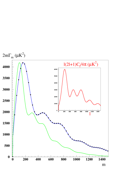
Figure 1: ’Typical’ power spectra. The insert shows a $\ell(2\ell+1)C_{\ell}/4\pi$ spectrum up to $\ell=1500$. The main graphs are two Fourier spectra ($2m\Gamma_{m}$) exactly calculated using Eq. 4 : one for $\Theta=90^{\circ}$ (darker curve), and the other for $\Theta=40^{\circ}$ (lighter curve). The triangles represent a subsample of the $2m\Gamma_{m}(\Theta=40^{\circ})$ coefficients after having rescaled their abscissa by a factor $1/\sin 40^{\circ}\ =\ 1.556$.

In this article, we present the scaling law and the inverse transformation that consists in the calculation of the $C_{\ell}$ from the $\Gamma_{m}$. In section 2, we demonstrate that this simple scaling law, displayed by the $m\Gamma_{m}$ spectrum for different colatitude angles, is accurate. Section 3 is dedicated to the description of two different methods proposed to invert Eq. 4 in the case $\Theta=90^{\circ}$. While a simple matrix inversion leads to the result, we also present an approximate analytic method. In section 4 these two methods are extended to the general case where $\Theta<90^{\circ}$.

2 Scaling of the $\mn@boldsymbol{m\Gamma_{m}(\Theta)}$ spectrum

Our study was triggered by one of us noticing that the product $m\Gamma_{m}(\Theta)$ is only function of the reduced variable $\mu\equiv{m}/{\sin\Theta}$, i.e. this product is independent (to a very good approximation) of the colatitude angle $\Theta$.

This scaling is illustrated in Fig. 1 where a $2m\Gamma_{m}$ spectrum computed for a colatitude angle of $\Theta\ =\ 40^{\circ}$ is scaled to match the corresponding $\Theta\ =\ 90^{\circ}$ one. To quantify the precision of this approximate scaling law, we have computed the differences between the scaled $2m\Gamma_{m}(\Theta)$ and the interpolated $2m\Gamma_{m}(\Theta=90^{\circ})$ spectrum (at $m/\sin\Theta$). Examples are shown in Fig. 2 for five $\Theta$ values ranging between $60$ and $10^{\circ}$. The absolute values of these differences are lower than $2\ \mu K^{2}$ over the whole $m$ range for the particular spectrum given in figure 1. They are only defined for $m$ values greater than $2/\sin\Theta$, as shown in the insert. Oscillations are observed in the difference. They present the same period but their amplitudes increase as the colatitude angle $\Theta$ decreases.

Different $2m\Gamma_{m}(\Theta)$ sets obtained from several detectors over a small range of colatitude angles $\Theta$ (a few degrees) may be combined using this scaling law, with a precision better than 0.01% . Several experiments, spanning a wider range of colatitude angles, may also be combined likewise, however with a slightly worse precision.

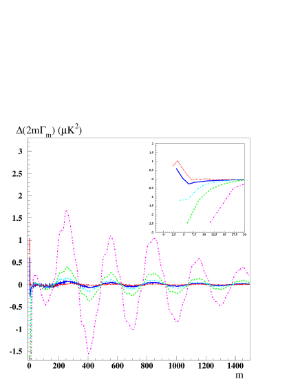
Figure 2: Absolute differences (in $\mu K^{2}$) between $2m\Gamma_{m}(\Theta)$ spectra scaled to $\Theta\ =\ 90^{\circ}$ and the interpolated $2m\Gamma_{m}(\Theta=90^{\circ})$ spectrum. All spectra are based on the $C_{\ell}$ spectrum of Fig.1. We have worked out these differences for $\Theta\ =\ 60^{\circ}$ (smallest amplitude curve), $40^{\circ}$, $30^{\circ}$, $20^{\circ}$ and $10^{\circ}$ (largest amplitude curve). The insert displays the low $m$ part, showing that the difference has a meaningful value only above $m=2/\sin\Theta$.

In the following, we explain this scaling law using a geometrical and a mathematical argument.

2.1 Geometric interpretation

The power spectrum $\Gamma_{m}(\Theta)$ is the Fourier transform of the signal autocorrelation function $A(\delta\phi,\Theta)$, where $\delta\phi$ is the phase difference between two points of the scanned ring. Two such points have an angular separation $\delta\psi$ on the unit sphere, where:

$$\delta\psi=2\arcsin(\sin\Theta\ \sin\frac{\delta\phi}{2})\,.$$ (5)

This relation between $\delta\phi$ and $\delta\psi$ allows one to express the scaling law, since the signal autocorrelation function, expressed as a function of $\delta\psi$ is equal to the autocorrelation function on a large circle scan:

$$A(\delta\psi,\pi/2)=A(\delta\phi,\Theta)\,.$$ (6)

For small $\delta\phi$, this relation becomes linear:

$$\delta{\psi}=\sin\Theta\ \delta\phi\,.$$ (7)

So that, in this linear regime, the autocorrelation function satisfies:

$$A(\delta\phi,\Theta)=A(\sin\Theta\ \delta\phi,\pi/2)\,.$$ (8)

Since the ring length $L$ on the unit sphere is $2\pi\sin\Theta$, the $m^{\rm{th}}$ harmonic of the Fourier expansion corresponds to structures on the sky of angular size

$$\lambda\equiv 2\pi\frac{\sin\Theta}{m}=\frac{2\pi}{\mu}\,.$$ (9)

In the continuum approximation, taking the Fourier transform of both sides of Eq. 8 leads to:

$$\Gamma_{m}(\Theta)=\frac{1}{\sin\Theta}\ \Gamma_{m/\sin\Theta}(\pi/2)\,,$$ (10)

which, using Eq.  9 leads to the scaling law:

$$m\Gamma_{m}(\Theta)=\mu\Gamma_{\mu}(\pi/2)\,.$$ (11)

While we are mainly concerned here with circular scanning, the same reasoning can be made for any kind of trajectory on the sky as long as it stays ‘close’ to a large circle on angular scales of order $\lambda$, and the same scaling law applies to the power density spectrum expressed as a function of ${1/\lambda}$.

2.2 Analytic interpretation

To investigate this scaling mathematically, we start from Eq. 4 which gives the exact relations that connect the $\Gamma_{m}(\Theta)$ to the $C_{\ell}$. Since the $B_{\ell}$ are – supposedly – well known quantities for each experimental set up, we will no longer mention them explicitly and we will deal with the coefficients $\mathcal{C}_{\ell}\equiv C_{\ell}B_{\ell}^{2}$.

We calculate the $\mathcal{P}_{\ell m}^{2}(\cos\Theta)$ factors using approximate expressions of the Legendre’s associated functions given by Robin (1957) (see appendix A for some details) which, once normalized, read

$\bullet$ for $\ell<m/\sin\Theta\,$:

$$\mathcal{P}_{\ell m} (\cos\Theta) \simeq\frac{1}{2\pi}\sqrt{\frac{\ell+\frac{1}{2}}{M}}\left(\frac{\ell\cos\Theta+M}{\ell}\right)^{\ell+\frac{1}{2}}$$

$$\times \left(\frac{m\cos\Theta-M}{(\ell-m)\sin\Theta}\right)^{m}\prod_{k=1}^{m}\sqrt{\frac{\ell+k-m}{\ell+k}}\,,\;\hskip 1.42271pt(12\rm{a})$$

where $M=\sqrt{m^{2}-\ell^{2}\sin^{2}\Theta}$,

$\bullet$ and for $\ell>m/\sin\Theta\,$:

$$\mathcal{P}_{\ell m}(\cos\Theta)\simeq\frac{(-1)^{m}}{2\pi}\sqrt{\frac{2(2\ell+1)}{N}}\cos\omega\,,\hskip 58.32823pt(12b)$$

where $N=\sqrt{l^{2}\sin^{2}\Theta-m^{2}}$. The expression of the angle $\omega$ is given in appendix A. These approximations are illustrated by Fig. 3.

For $\ell<m/\sin\Theta$, the numerical value of $\mathcal{P}_{\ell m}^{2}(\cos\Theta)$ is negligible, while for $\ell>m/\sin{\Theta}$  Eq. 6b implies

$$\mathcal{P}_{\ell m}^{2}(\cos\Theta)\simeq\frac{1}{4\pi^{2}}\frac{2\ell+1}{(\ell^{2}\sin^{2}\Theta-m^{2})^{1/2}}[1+\cos(2\omega)]\,.$$ (13)

Since the CMB angular power spectrum varies slowly as a function of $\ell$, we may replace the sum over $\ell$ in Eq. 4 by an integral. We thus obtain

$$m\Gamma_{m}(\Theta)=\frac{m}{4\pi^{2}}\int_{\frac{m}{sin\Theta}}^{\ell_{max}}\!\frac{\mathcal{C}(\ell)[2\ell+1][1+\cos(2\omega)]}{(\ell^{2}\sin^{2}\Theta-m^{2})^{1/2}}\ \,d\ell\,$$ (14)

where $\ell_{max}$ is an $\ell$ value beyond which the power spectrum vanishes, and $\mathcal{C}(\ell)$ is a function of $\ell\,\in\>]0,\ell_{max}]$ that smoothly interpolates the $\mathcal{C}_{\ell}$ coefficients (a simple way of proceeding is given in Appendix B).

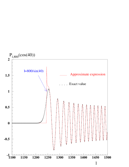
Figure 3: Comparison between the exact value of $\mathcal{P}_{\ell\>800}(\cos(40^{\circ}))$ as a function of $\ell$, dotted line, and the one obtained with the approximate expressions of Eqs. (12a) and (12b), solid line. The arrow indicates the $\ell\ =800/\sin{40^{\circ}}$ abscissa.

The oscillation frequency $\nu$ of the cosine term (as a function of $\ell$) in the integrand in the right side of Eq. 14 is of order $\Theta/\pi$ (thus $\nu\sim 1/2$ when $\Theta=\pi/2$). Such a frequency is high enough for this cosine term to contribute to a very small amount to the integral. This will be checked numerically in section 3.1 below. Thus we may write:

$$m\Gamma_{m}(\Theta)\simeq\frac{1}{4\pi^{2}}\int_{\mu}^{\ell_{max}}\mathcal{C}(\ell)\frac{2\ell+1}{[(\ell/\mu)^{2}-1]^{1/2}}\,d\ell\;.$$ (15)

This equation demonstrates – within the approximations that have been made – that the product $m\Gamma_{m}(\Theta)$ depends only on the variable $\mu={m}/{\sin\Theta}$.

Since the variable $\mu$ is not constrained to be an integer, one has to introduce a smooth function, $\Gamma(m,\Theta)$ where $m$ is now a real, that interpolates the $\Gamma_{m}(\Theta)$ discrete spectrum. This can be done in the same way as the one indicated for the $\mathcal{C}_{\ell}$ spectrum (cf. Appendix B).

In terms of this $\Gamma(m,\Theta)$ function, the scaling law is expressed by the relation:

$$\Gamma(m^{\prime},\Theta^{\prime})=\frac{\sin\Theta}{\sin\Theta^{\prime}}\Gamma(m^{\prime}\frac{\sin\Theta}{\sin\Theta^{\prime}},\Theta)\,.$$ (16)

This equation follows from the equality $m\Gamma(m,\Theta)=m^{\prime}\Gamma(m^{\prime},\Theta^{\prime})$ which holds true provided that $m/\sin\Theta=m^{\prime}/\sin\Theta^{\prime}$.

Assuming that the Fourier spectrum has been obtained for a particular value $\Theta$ of the colatitude angle, Eq. 16 allows one to calculate $\Gamma(m^{\prime},\Theta^{\prime})$ for $m^{\prime}=m\sin\Theta^{\prime}/\sin\Theta,\;m=1,2\cdots m_{max}=\ell_{max}\sin\Theta$. Then, by interpolation, one gets $\Gamma(m^{\prime},\Theta^{\prime})$ for all integer values of $m^{\prime}$ ranging from $\sin\Theta^{\prime}/\sin\Theta$ up to $\ell_{max}\sin\Theta^{\prime}$. Eq. 16 can thus be used to compare and combine Fourier spectra that correspond to different $\Theta$ values.

3 Recovering the $\mn@boldsymbol{\mathcal{C}_{\ell}}$ coefficients from the $\mn@boldsymbol{\Gamma_{m}(\pi/2)}$ Fourier spectrum

3.1 Checking and solving the integral equation that relates $\mn@boldsymbol{\mathcal{C}(\ell)}$ to $\mn@boldsymbol{\Gamma(m,\pi/2)}$

Since $\Theta$ is assumed to be equal to $\pi/2$ in this section, the variable $\mu$ can be identified with $m$.

In order to facilitate the numerical calculation of the right side of Eq. 15, we introduce a new variable of integration $x$ defined by $\ell=m\cosh x$. Then Eq. 15 can be rewritten

$$\Gamma(m,\pi/2)=\frac{1}{4\pi^{2}}\int_{0}^{\cosh^{-1}(\ell_{max}/m)}(2m\cosh x+1)\mathcal{C}(m\cosh x)\;dx\,.$$ (17)

The transformation defined by Eq. 17 is linear: thus one may insert in the integrand an interpolating function of the $\mathcal{C}_{\ell}$ spectrum as defined by Eq. 33. The output of Eq. 17 applied to the angular power spectrum of Fig. 1 is shown in Fig. 4. One can see in this Fig. 4 that for such a spectrum the approximations that were made in section 2 ensure an accuracy better than 1% – except at the lower end of the spectrum where the relative error drops below $2$ % for $m=14$.

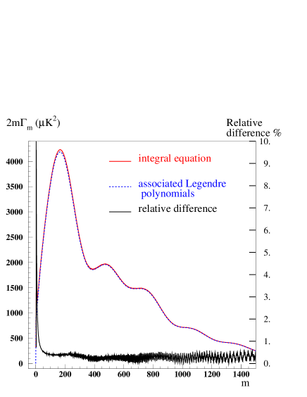
Figure 4: Comparison between the $2m\Gamma_{m}$ coefficients computed with the associated Legendre’s polynomials (dashed line) and the $2m\Gamma(m)$ function calculated using Eqs. 17, 33 and 34 with $\sigma=0.5$ (solid line). The relative difference between the results of the two calculations is shown by the lower curve (in %, right scale).

Eq. 17 can be solved for $\mathcal{C}(\ell)$ by noticing that this integral equation is similar to Schlömilch’s equation which reads

$$F(m)=\frac{2}{\pi}\int_{0}^{\pi/2}\Phi(m\sin x)\;dx$$ (18)

where $m$ is a real.

The way to solve the latter equation can be found e.g. in Kraznov (1977). We proceed in a similar way for Eq. 17 (the details are given in Appendix C) and we obtain

$${\mathcal{C}({\ell})=-8\pi\frac{\ell}{2\ell+1}\int_{0}^{\cosh^{-1}(\ell_{max}/\ell)}\Gamma^{\prime}(\ell\cosh x)\;dx}\,,$$ (19)

where $\Gamma^{\prime}$ is the derivative of $\Gamma(m,\pi/2)$ with respect to $m$. Again the transformation implied by Eq. 19 is a linear one, allowing the use of interpolating functions as defined in Appendix B. Fig. 5 illustrates the use of this integral equation to calculate the $\mathcal{C}_{\ell}$ coefficients starting with the set of $\Gamma_{m}(\pi/2)$’s.

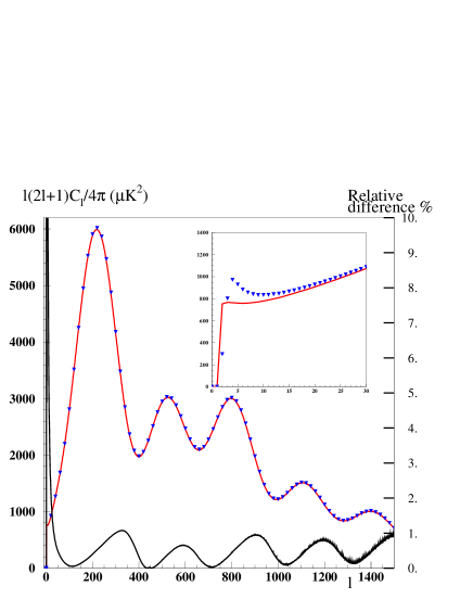
Figure 5: Comparison between the ’Typical’ $\mathcal{C}_{\ell}$ coefficients for $\Theta=90^{\circ}$ (solid line), used to calculate the $\Gamma_{m}$ Fourier spectrum (using the $\mathrm{\mathbf{P(0)}}$ matrix) and the $\mathcal{C}(\ell)$ function obtained by inserting this Fourier spectrum in Eq. 19, (triangles; only some points are shown). We have set $\sigma=1$ in Eq. 34. The relative difference (in %) is shown by the lower curve (right scale). Insert: zoom on the low $\ell$ region.

3.2 Numerical inversion

In the $\Theta={\pi}/{2}$ case, the connection between the set of $C_{\ell}$’s and the corresponding $\Gamma_{m}$’s is simple since Eq. 4 can be written using matrices (M. Piat et al. 2002):

$$\vec{\Gamma}=\mathrm{\mathbf{P(0)}}\times\vec{\mathcal{C}}\,,$$ (20)

with:

$$\mathrm{\mathbf{P(0)}}_{ij}=\left[{\cal P}_{ji}(0)\right]^{2},$$ (21)

where ${\cal P}_{ji}$ are the normalized associated Legendre’s functions. $\mathrm{\mathbf{P(0)}}$ is (upper) triangular.

In addition, since the associated Legendre polynomials are defined as:

$$P_{\ell m}(0)=\begin{cases}(-1)^{p}\frac{(2\ell+2m)!}{2^{\ell}p!(p+m)!}&\mbox{if\ $\ell-m=2p$}\hskip 28.45274pt\mbox{[a]},\\ 0&\mbox{if\ $\ell-m=2p+1$}\hskip 12.80365pt\mbox{[b]},\end{cases}$$ (22)

all of the $\mathrm{\mathbf{P(0)}}_{ii}$ diagonal elements are different from zero – thus this matrix is invertible.

The inverse of $\mathrm{\mathbf{P(0)}}$ is also upper triangular and keeps the peculiar structure of the original matrix: in both $\mathrm{\mathbf{P(0)}}$ and $\mathrm{\mathbf{P(0)}}$ ​​^-1 only the $\ell-m=2p$ terms differ from zero.

3.3 Comparison between the analytic and the numerical transformations

One way of comparing the two methods of calculating the Fourier spectrum is to look at what happens when a single $\mathcal{C}_{\ell}$ coefficient is different from zero. This is done in Fig. 6 for the case where $\mathcal{C}_{300}=1$. Note that since we assume here that $\Theta={\pi}/{2}$, Eq. 22 b implies that all $\Gamma_{m}$ coefficients with an odd index vanish (for a single non vanishing $C_{\ell}$ coefficient with an odd $\ell$ value, all $\Gamma_{m}$ coefficients with an even index would vanish). One notices that the $\Gamma(m)$ function runs at mid-height of the non-vanishing $\Gamma_{m}$ coefficients.

Conversely, one may look at the $\mathcal{C}(\ell)$ function that corresponds to the case where a single $\Gamma_{m}$ Fourier coefficient is different from zero as shown in Fig. 7 (here we used $\Gamma_{300}\neq 0$). The fact that the $\mathcal{C}(\ell)$ graph is negative in some domain of $\ell$ values shows that no distribution of temperature inhomogeneities which satisfies the validity conditions of Eq. 4 (isotropy and Gaussian $a_{\ell m}$) can correspond to a Fourier spectrum with a single non-vanishing coefficient.

Taken together, Figs. 6 and 7 show where we should expect a strong signal in one spectrum in the case the other spectrum presents a high power in some particular bins.

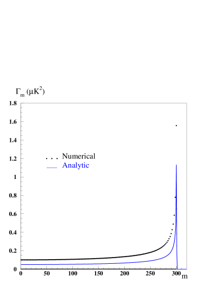
Figure 6: Middle curve (solid line) : Fourier spectrum obtained using Eq. 17 when only $\mathcal{C}_{300}\neq 0$. We have used $\sigma=0.5$ in Eq. 34. Upper and lower set of points: the $\Gamma_{m}$ coefficients computed with the $\mathrm{\mathbf{P(0)}}$ matrix. Since we assume here that $\Theta=\pi/2$, all $\Gamma_{m}$ coefficients whose indexes $m$ are odd vanish.

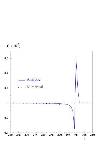
Figure 7: Solid line: the $\mathcal{C}_{\ell}$ spectrum obtained with Eq. 19 when only $\Gamma_{300}\neq 0$ (we have set $\sigma=1$ in Eq. 34). In dots: the $C_{\ell}$ coefficients calculated with the $\mathrm{\mathbf{P(0)}}$ ​​^-1 matrix .

4 Working with smaller rings on the sky ($\mn@boldsymbol{\Theta<\pi/2}$)

4.1 General features of the Fourier spectrum

In the preceding section we assumed that the scanned rings are the largest ones on the sphere ($\Theta={\pi}/{2}$). In this case the fact that the $\mathrm{\mathbf{P(0)}}$ matrix is invertible establishes that the Fourier spectrum of such rings contains all the physical information carried by the $\mathcal{C}_{\ell}$ coefficients.

Scanning smaller circles on the sky implies a higher fundamental frequency in Fourier angular space and thus a less dense sampling of this Fourier space.

In fact the loss of information is then twofold:

• The $G(\mu)\equiv m\Gamma(m,\Theta)$ function is no longer measured for $\mu=1$: the lowest value of $\mu$ which can be reached with the data is now $\mu={1}/{\sin\Theta}$.

• Secondly, $G(\mu)$ is no more measured for $\mu$ values that differ by one but for $\mu$ values that differ by ${1}/{\sin\Theta}$. As a very simple example: if the scan is performed for $\Theta={\pi}/{6}$, then one measures $G(\mu)$ only for $\mu=2n$ with $n\,\in\,]0,\ell_{max}/2]$. Because of the smoothness of the angular spectra, this sparse sampling of the function $G(\mu)$ is not necessarily a drawback as long as the accuracy of the measurements compensates for it.

4.2 Analytic calculation of the $\mn@boldsymbol{\mathcal{C}_{\ell}}$ spectrum for $\mn@boldsymbol{\ell>1/\sin\Theta}$

As far as the analytic calculation of the $\mathcal{C}_{\ell}$ spectrum is concerned, it can be performed with the same formalism as above (cf. subsection 3.1). One should merely replace the derivative of $\Gamma(m,\pi/2)$ that appears in the right side of Eq. 19 by the derivative (with respect to $m$) of

$$\tilde{\Gamma}(m)=\sin\Theta\sum_{i=1}^{\ell_{max}\sin\Theta}\Gamma_{i}f(m\sin\Theta-i)\,.$$ (23)

$\tilde{\Gamma}(m)$ is just the rescaled version (cf. Eq. 16) of $\Gamma(m,\Theta)$ defined by Eq. 35 (this rescaling translates the $\Gamma(m,\Theta)$ Fourier spectrum into the one corresponding to $\Theta=\pi/2$). Furthermore the width of the interpolating function $f(x)$ of Appendix B (see Eq. 34) should be increased by a factor ${1}/{\sin\Theta}.$

4.3 Numerical calculation of the $\mathcal{C}_{\ell}$ spectrum for $\ell>1/\sin\Theta$

It follows from subsection 4.1 above that the $\Gamma_{m}(\Theta)$ coefficients differ significantly from zero in the range $1\leq m\leq\ell_{max}\sin\Theta$. Then using the $\Gamma(m,\Theta)$ function that interpolates these coefficients and Eq. 16 one can calculate the following set of $\ell_{max}-\ell_{min}+1$ values

$$\tilde{\Gamma}_{m^{\prime}}=\sin\Theta\ \Gamma(m^{\prime}\sin\Theta,\Theta),$$ (24)

with $m^{\prime}=\ell_{min},\,\ell_{min}+1,\cdots\ell_{max}$ where $\ell_{min}$ is the first integer larger than $1/\sin\Theta$. These $\tilde{\Gamma}_{m^{\prime}}$ coefficients are the ones of the Fourier spectrum for $\Theta=\pi/2$. Once obtained, the $C_{\ell}$ spectrum is simply given by

$$\vec{\mathcal{C}}=\mathrm{\mathbf{P(0)}}^{-1}\vec{\tilde{\Gamma}}\,$$ (25)

for $\ell\geq\ell_{min}$. The $\mathrm{\mathbf{P(0)}}$ matrix and its inverse have been discussed in section 3.2. The first $\ell_{min}-1$ rows and columns of $\mathrm{\mathbf{P(0)}}^{-1}$ should be omitted in Eq. 25 since the lowest value of the $m^{\prime}$ index is $\ell_{min}$.

Fig. 8 shows a numerical example: we use the ‘typical’ $C_{\ell}$ spectrum of Fig. 1, to produce a set of $\Gamma_{m}$ values in the $\Theta=40^{\circ}$ case (Eq. 4). Then we apply the method described above and compare the input spectrum to the obtained one. In this example we used a simple linear interpolation of the $\Gamma_{m}$ spectrum. The agreement is excellent and better than the one obtained with the analytic method (cf. Fig. 5) as the latter involves some approximations (cf. section 2) in addition to the ones stemming from the scaling and the interpolation procedure.

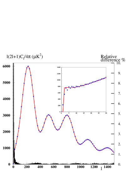
Figure 8: The input $C_{\ell}$ spectrum (solid curve) and the one reconstructed by the numerical method in the $\Theta=40^{\circ}$ case (only some points are shown). The relative difference between the two spectra is shown by the lower curve (in %, right scale). Insert : zoom on the low $\ell$ region.

The excellent agreement of Fig. 8 breaks down for low values of $\ell$. Nevertheless, for $\ell\gtrsim 3$ in the $\Theta=40^{\circ}$ case, one gets an agreement better than 10% (far above the cosmic variance). For the case $\Theta=80^{\circ}$ our simple scaling method can be used up to an accuracy better than 1% for any $\ell$ values.

5 Conclusion

We have shown how data taken on circles with different colatitude angle $\Theta$ can be combined using a scaling law that is satisfied by the $m\Gamma_{m}(\Theta)$ coefficients at the $0.1$ % level in a wide range of $m$ and $\Theta$ values.

Then we have derived this scaling property from both geometrical considerations and linear expressions of the $\Gamma_{m}$ coefficients in terms of the $C_{\ell}$ ones by introducing analytic approximations of the normalized Legendre’s associated polynomials $\mathcal{P}_{\ell m}(\cos\Theta)$ that enter these relations.

Integral equations were obtained that relate to a good approximation interpolating functions of the two sets of coefficients ($\Gamma_{m}$ and $C_{\ell}$). These analytic relations give a simple picture of the connection between the two types of spectra and are easy to use.

Finally we have investigated ways of calculating the $C_{\ell}$ coefficients when the $\Gamma_{m}$ Fourier spectrum is known. We have shown how the inverse of the $\mathcal{P}_{\ell m}^{2}(0)$ matrix can be used to perform this calculation not only for $\Theta=\pi/2$ but also in the general case where $\Theta<\pi/2$. This was achieved by taking advantage of the scaling of the $m\Gamma_{m}$ spectrum on the one hand and of its smoothness on the other.

This set of results provides a basis for further investigation of the connection between the measured $C_{\ell}$ and $\Gamma_{m}$ spectra altered by noise and errors.

Appendix A Approximate expressions of the normalized Legendre’s associated polynomials

We start with asymptotic expressions of the Legendre’s functions obtained by  Robin (1957) in the limit of large $\ell$, ${m}/{\ell}$ being kept constant. These asymptotic expressions depend on the relative value of $m$ and $\ell\sin\Theta$.

$\bullet$ For $\ell<m/\sin\Theta$,

$$P_{\ell m}(\cos\Theta)\simeq$$

$$\frac{(-1)^{m}\ell!}{\sqrt{2\pi}(\ell-m)!} \frac{(\ell\cos\Theta+M)^{\ell+\frac{1}{2}}(m\cos\Theta-M)^{m}}{\ell^{\ell+\frac{1}{2}}(\ell-m)^{m}M^{\frac{1}{2}}\sin^{m}\Theta}\,,$$ (26)

where $M=\sqrt{m^{2}-l^{2}\sin^{2}\Theta}\,,$

$\bullet$ while for $\ell>m/\sin\Theta$,

$$P_{\ell m}(\cos\Theta)\simeq$$

$$(-1)^{m}\sqrt{\frac{2}{\pi}} \frac{\ell!(\ell-m)^{\frac{\ell-m}{2}+\frac{1}{4}}(\ell+m)^{\frac{\ell+m}{2}+\frac{1}{4}}}{(\ell-m)!\ell^{\ell+\frac{1}{2}}N^{\frac{1}{2}}}\cos\omega$$ (27)

where

$$N = \sqrt{\ell^{2}\sin^{2}\Theta-m^{2}}\,,$$ (28)

$$\omega = (\ell+\frac{1}{2})\alpha-m\beta-\frac{\pi}{4}\,,$$ (29)

$$\alpha = arg(\ell\cos\Theta+iN)\,,$$ (30)

$$\beta = arg(m\cos\Theta+iN)\,.$$ (31)

To ‘normalize’ these polynomials and obtain the $\mathcal{P}_{\ell m}$ ones, they must be multiplied by

$$\sqrt{\frac{2\ell+1}{4\pi}\frac{(\ell-m)!}{(\ell+m)!}}.$$ (32)

Then the last step consists in using Stirling’s formula ($n!\simeq\sqrt{2\pi}\,n^{n+\frac{1}{2}}\,e^{-n}$) to replace the factorials by analytic functions. A few simplifications can then be made that lead to the approximate expressions used in section 2.

Appendix B Interpolating functions of the discrete power spectra

Since the calculation of the $C_{\ell}$ coefficients involves integrals over spherical Bessel $j_{\ell}$ functions (see, e.g. Seljak U. & Zaldarriaga 1996), one may try and use an expression of these functions that extends them to non-integer values of $j$. But here we will adopt a much simpler procedure and write

$$\mathcal{C}(\ell)\equiv\sum_{i=1}^{\ell_{max}}\mathcal{C}_{i}f(\ell-i),$$ (33)

where $\ell$ is now a real whose value ranges between $2$ (recall that we ignore the dipole term) and $\ell_{max}$, and $f(x)$ is a positive, infinitely differentiable function ($f\in\,{\cal C}^{\infty}$), which differs significantly from $0$ in an $|x|$ range which is of order unity, and whose integral over $x$ is unity. In practice we used

$$f(x)=\frac{1}{\sqrt{2\pi}\,\sigma}\exp{\frac{-x^{2}}{2\sigma^{2}}}$$ (34)

with $\sigma\sim 1$.

Similarly, we define an interpolating function for the $\Gamma_{m}(\Theta)$ coefficients in the following way:

$$\Gamma(m,\Theta)\equiv\sum_{i=1}^{\ell_{max}\sin\Theta}\Gamma_{i}f(m-i),$$ (35)

where $m$ is a real and $f(x)$ is chosen as above.

Appendix C Inversion of the integral equation relating $\mn@boldsymbol{\mathcal{C}(\ell)}$ to $\mn@boldsymbol{\Gamma(m)}$

Since $\mathcal{C}(\ell)$ vanishes for $\ell>\ell_{max}$, the integral equation (17) is of the form

$$\Gamma(m)=\int_{0}^{\infty}h(m\cosh x)\;dx\,.$$ (36)

We differentiate both sides of this equation with respect to $m$, substitute for this variable $m$ the product $u\cosh\psi$, and integrate both sides over $\psi$ between the limits $0$ and $\infty$. We thus obtain:

$$\int_{0}^{\infty}\!\!\!\!\!\!\Gamma^{\prime}(u\cosh\psi)\>d\psi=\!\!\!\int_{0}^{\infty}\!\!\!\!\!\!dx\!\int_{0}^{\infty\!}\!\!\!\!\!h^{\prime}(u\cosh\psi\cosh x)\cosh x\>d\psi.$$ (37)

Then a new integration variable $\xi$ is used in the second integral of the right side of this equation, defined by $\cosh\xi=\cosh\psi\cosh x$. Some simple algebra then leads to

$$\int_{0}^{\infty}\!\!\!\!\!\!\Gamma^{\prime}(u\cosh\psi)d\psi=\!\!\!\int_{0}^{\infty}\!\!\!\!\!\!dx\int_{x}^{\infty}\!\!\frac{h^{\prime}(u\cosh\xi)\sinh\xi\cosh x}{\sqrt{\sinh^{2}\xi-\sinh^{2}x}}d\xi.$$ (38)

Once the integration order is reversed in the right side of this equation on obtains:

$$\int_{0}^{\infty}\Gamma^{\prime}(u\cosh\psi)\;d\psi=\int_{0}^{\infty}h^{\prime}(u\cosh\xi)\sinh\xi d\xi$$

$$\int_{0}^{\xi}\frac{\cosh x\;dx}{\sqrt{\sinh^{2}\xi-\sinh^{2}x}}.$$ (39)

The integral over $x$ is simply ${\pi}/{2}$. Furthermore $h(\infty)=0$ in our case, so that

$$h(u)=-\frac{2u}{\pi}\int_{0}^{\infty}\Gamma^{\prime}(\xi\cosh\psi)\;d\psi\,.$$ (40)

References

- ARCHEOPS (2002) ARCHEOPS: Benoît, A. et al. astro-ph/0210305 submitted
- Bond & Efstathiou (1987) Bond, J. R. & Efstathiou, G. 1987, MNRAS, 226, 655
- CBI (2002) CBI: Contaldi, C. R., Bond, J. R., Pogosyan, D., et al. preprint [astro-ph/0210303]
- Delabrouille et al. (1998) Delabrouille, J., Gorski, K. M.,& Hivon, E., 1998, MNRAS , 298, 445
- DASI (2002) DASI: Halverson, N. W., Leith, E. M., Pryke, C., et al. 2002, ApJ 568, 38
- MAXIMA (2000) MAXIMA: Hanany, S., Ade, P., Balbi, A. et al. 2000, ApJ, 545L, L5
- Hu & Dodelson (2002) Hu, W. & Dodelson,S. 2002, ARA& A, 40, 171
- Kraznov (1977) Kraznov, M et al., Equations intégrales, Editions de Moscou, 1977.
- BOOMERANG (2000) BOOMERANG: Mauskopf, P. D.,Ade, P. A. R., de Bernardis, P., et al. 2000, ApJ, 536L, L59
- M. Piat et al. (2002) M. Piat, G. Lagache, J.P. Bernard, M. Giard, and J.L. Puget, A& A 393,359-368,2002
- Robin (1957) Robin, L., Fonctions sphériques de Legendre et fonctions sphéroïdales, Gauthier-Villars (3 vol. 1957-1959)
- Seljak U. & Zaldarriaga (1996) Seljak, U. & Zaldarriaga M., 1996, A&A , 469, 437
- VSA (2002) VSA: Taylor, A. C., Carreira, P., Cleary, K., et al. preprint [astro-ph/0205381]