Abstract

In this paper we present numerical simulations of the evolution of planets or massive satellites captured in the 2/1 and 3/1 resonances, under the action of an anti-dissipative tidal force. The evolution of resonant trapped bodies show a richness of solutions: librations around stationary symmetric solutions with aligned periapses ($\Delta\varpi=0$) or anti-aligned periapses ($\Delta\varpi=\pi$), librations around stationary asymmetric solutions in which the periapses configuration is fixed, but with $\Delta\varpi$ taking values in a wide range of angles. Many of these solutions exist for large values of the eccentricities and, during the semimajor axes drift, the solutions show turnabouts from one configuration to another. The presented results are valid for other non-conservative forces leading to adiabatic convergent migration and capture into one of these resonances.

EVOLUTION OF MIGRATING PLANET PAIRS IN RESONANCE

S.Ferraz-Mello , C.Beaugé and T.A.Michtchenko

Keywords: exoplanets, Galilean satellites, resonance, planetary migration, tidal forces.

1 Introduction

The present paper considers the problem of a pair of planets (or planetary satellites) captured in the 2/1 and 3/1 mean-motion resonances, in which the inner mass is under the action of an anti-dissipative force that continuously increases its semimajor axis. Convergent migration of bodies and the action of non-conservative disturbing forces are subjects that have been explored by many authors (for a recent publication and bibliographical list, see Jancart 2002). However, in almost all those studies, one of the bodies is assumed to have negligible mass and does not exert any gravitational action on the rest of the system. The scenario usually considered is thus the restricted three-body problem to which a non-conservative force is added. In this work, we are interested in systems where the two planets (or satellites) have finite masses. As examples of such systems, we may cite some of the newly discovered extrasolar planetary systems (e.g. Gliese 876, HD82943, 55 Cnc) and, in our Solar System, some satellite pairs such as Io-Europa or Europa-Ganymede. Even if we expect a phenomenology showing many of the characteristics seen in the restricted models, only actual calculations can tell us how much of the dynamics is equivalent and, if not, which are the main changes.

The paradigm of a system of finite mass bodies captured into resonance is the system formed by the three inner Galilean satellites of Jupiter. If we denote by $\lambda_{1}$, $\lambda_{2}$ and $\lambda_{3}$, the mean longitude of Io, Europa and Ganymede, respectively, it was shown by Laplace that the motion of these bodies is such that the angle

$$\lambda_{1}-3\lambda_{2}+2\lambda_{3}$$

oscillates around $\pi$ with a small amplitude, $\sim 10^{-3}$ rad (Lieske, 1998). Laplace also investigated the effect of a perturbation leading to an acceleration of the mean longitudes of one of the satellites. He showed that the mutual interaction of the three satellites would redistribute the effect among all the longitudes in such a way that the libration of the angle $\lambda_{1}-3\lambda_{2}+2\lambda_{3}$ around $\pi$ would be conserved (see Tisserand 1896, Ferraz-Mello 1979). Nonetheless, the current tidal acceleration of the Galilean satellites is very small. Modern determinations of the rate acceleration/velocity, as deduced from old satellite eclipses and recent mutual events observations, are $(2.88\pm 0.10)\times 10^{-10}{\rm yr}^{-1}$ (Aksnes and Franklin 2000) and $(-0.074\pm 0.087)\times 10^{-10}{\rm yr}^{-1}$ (Lieske 1987). Heat dissipation observed on the surfaces of Io and Europa indicates that tides raised by Jupiter on the satellites are among the main dissipative agents at work in this system (see Yoder, 1979).

More recently, several resonant extrasolar planetary systems have been discovered with dynamical features suggesting that they have undergone a large-scale migration. In most cases, this orbital migration is believed to be due to an interaction of the planets with a residual planetesimals disk. In some extreme cases, tides have also been considered among the sources of orbital evolution; this seems to be the case of the putative planetary system around HD 83443 (Wu and Goldreich, 2002) where the inner planet has the smallest semimajor axis among all currently known exoplanets. However, recent observations have not confirmed the existence of a pair of planets around that star. It is worth noting that many of the discovered exoplanets, including the inner planet of $\upsilon\,$And, orbit at distances smaller than 0.077 AU where tidal interaction with the central star should be important. All these planets are candidates to have an initial dynamical evolution similar to that shown by the Jupiter-Io system.

In this paper, we present a series of numerical simulations of the dynamical evolution of planetary satellites due to tidal effects, concentrating on the orbital variation after a capture in the 2/1 and 3/1 mean-motion resonances. Except for a change in the timescale of the process, these results should also be representative of the evolution of extrasolar planets moving very close to the central star.

2 2-body tidal interaction

The anti-dissipative force used in this paper corresponds to tides raised on the central mass $m_{0}$ (star or planet) by an orbiting body $m_{1}$ (planet or satellite). In addition, $m_{1}$ is interacting with a similar body $m_{2}$ placed in an orbit external to that of $m_{1}$. The model is planar and the spin axis of the central mass is assumed normal to the orbital plane. The two secondary bodies have finite masses but their sizes are neglected; they are thus considered as mass points. We will further assume that the tidal interaction only affects the inner body and not the outer one. This is, by far, our most stringent hypothesis. Tidal forces are inversely proportional to the $7^{\,\rm th}$ power of the distance to the central body; at the beginning of our simulations, we always considered ${a_{1}}/{a_{2}}<0.6$, making the tidal interaction of the outermost orbiting body $10^{2}$ times smaller, but in simulations where the bodies escape an early capture and ${a_{1}}/{a_{2}}$ grows significantly, the results of a simulation taking into account both tidal interactions may be very different.

Before presenting the physics of the used model, we should stress that the results presented in this paper were obtained in the frame of a more general investigation of the interplay of tides and resonance amongst finite mass bodies. For this reason, no averaging of the forces was used. Averaged equations are fine tools to assess the main effects in restricted there-body problems, but are less confident when a third massive body is interacting with the other two. The reason is simple: the averaged equations inside and outside resonances are not the same (see Ferraz-Mello, 1987). In a general problem, the semi-major axes have secular variations, resonance zones are crossed, one after another, and new phenomena are likely to occur which may not appear if the equations are, in some way, simplified.

In view of this, the experiments presented in this work were performed via numerical simulations of the exact equations. Although more accurate, this approach leads to new problems. Since realistic tidal effects introduce extremely slow orbital variations, the integration times are prohibitive. Consequently, we have been obliged to enhance these perturbations to be able to obtain significant variations in the system, in reasonable integration times. In all our simulations, we increased the value of the ratio

$$\chi=2\Delta t(\Omega-n)$$ (1)

by some 2 or 3 orders of magnitude. Here, $\Delta t$ is the tide time lag, $\Omega$ is the rotation angular velocity of the extended body where the tide is raised and $n$ the orbital mean motion of the tidally interacting two-body system. The consequence is an acceleration of the evolutionary timescale by the same factor increasing $\chi$. However, this is not a real scaling of the problem because the factor $\chi$ only enters in one of the right-hand side terms of the equations of motion. It is important to keep in mind that the increase of $\chi$ must not be taken too large; the interplay of the migration due to the tide and one resonance depends on the speed with which the resonance is crossed, and the probability of capture at a crossed resonance lessens as $\chi$ grows. However, in this paper, we are more interested in the phenomena taking place after a capture, which are less affected by the enhancement of $\chi$ as long as this does not introduce large forced oscillations about stable stationary solutions.

2.1 Tidal forces

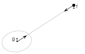
Figure 1: Interaction of an extended body and a mass point.${\bf f}$ and ${\bf g}$ represent the resultant of the forces due to tides raised by the mass point on the extended body.

Consider a mass point $m_{1}$ raising tides on an extended body of mass $m_{0}$. Let ${\bf r}$ be the radius vector of $m_{1}$ relative to $m_{0}$. The big arrows in figure 1, show the central attraction forces between both masses, while $\mathbf{f},\,\mathbf{g}$ are the resultants of the forces due to the tidally deformed shape of $m_{0}$. Since the system of forces is in equilibrium they satisfy to the relation ${\mathbf{f}=-\mathbf{g}}$. According with the Darwin-Mignard tidal model (Mignard 1981), we have:

$${\mathbf{f}}=-{\displaystyle{3k_{2}\Delta t\frac{Gm_{1}^{2}R_{0}^{5}}{r^{10}}}}\left[2\mathbf{r}(\mathbf{r}\cdot\mathbf{v})+r^{2}(\mathbf{r}{\mathbf{\times}}\mathbf{\Omega}+\mathbf{v})\right]$$ (2)

where $R_{0}$ and $\mathbf{\Omega}$ are the equatorial radius and the angular rotation velocity (vector) of the extended body, $k_{2}$ is the tidal Love number and $\mathbf{v}=\dot{\mathbf{r}}$. We can easily compute the acceleration of the two bodies with respect to an inertial frame and subtract them to obtain the relative acceleration:

$$\ddot{\mathbf{r}}=-\frac{G(m_{0}+m_{1})\mathbf{r}}{r^{3}}+\frac{(m_{0}+m_{1}){\mathbf{f}}}{m_{0}m_{1}}$$ (3)

or

$$\ddot{\mathbf{r}}=-\frac{GM\mathbf{r}}{r^{3}}+\frac{\mathbf{f}}{m}$$ (4)

where $M=m_{0}+m_{1}$ is the total mass and $m$ is the reduced mass $m=\frac{m_{0}}{M}m_{1}$. If we assume that $m_{0}\gg m_{1}$, then $m\simeq m_{1}$ and $M\simeq m_{0}$.

2.2 The Torque on the Planet

The momentum of the couple shown in figure 1 is ${\mathbf{r}{\mathbf{\times}}\mathbf{f}}$. Since the system is isolated, this momentum must be compensated by the momentum of the forces acting internally on the extended body with respect to its center of mass:

$${\mathbf{T}=-\mathbf{r}{\mathbf{\times}}\mathbf{f}}.$$ (5)

The rotation angular momentum $\mathbf{S}$ of the extended body will then change following the law

$${\dot{\mathbf{S}}=\mathbf{T}}$$ (6)

or, if we assume that the momentum of inertia $I$ of the extended body about the rotation axis is constant,

$$I\dot{\mathbf{\Omega}}=\mathbf{T}$$ (7)

Introducing the expression for the force from equation (2), we obtain

$${\mathbf{T}}={\displaystyle{3k_{2}\Delta t\frac{Gm_{1}^{2}R_{0}^{5}}{r^{8}}}}\left[r^{2}\mathbf{\Omega}-(\mathbf{r}\cdot\mathbf{\Omega})\mathbf{v}+\mathbf{v}{\mathbf{\times}}\mathbf{r}\right].$$ (8)

Equations (7)-(8) give the temporal variation of the angular rotation velocity of the planet due to the tidal effects. In a series of preliminary simulations performed for the Jupiter-Io pair, we found that the perturbation is extremely small and the value of $\Omega$ remains practically unchanged. As an example, a typical run spanning 30 scaled Myrs (corresponding to 1.25 Gyr, considering the scaling of $\chi$) lead to a variation of the total orbital angular momentum of $\Delta S=+7.4\times 10^{-11}M_{\,\odot}{\,\rm AU}^{2}/yr$ and, consequently, a variation of the rotation period of Jupiter of only +8.8 seconds.

Following this result, for the rest of our calculations we will consider the rotation period of the extended body constant. Of course, a working hypothesis of this kind can only be adopted when the relative masses of the orbiting bodies to the central one are $<10^{-3}$, as in the Jupiter-Io and many planet-exoplanet cases. In cases such as the Earth-Moon pair (MacDonald 1964, Touma and Wisdom 1994), the mass ratio is much higher ($\sim 1/80$) and the rotation period variations should be computed together with those of the orbital parameters.

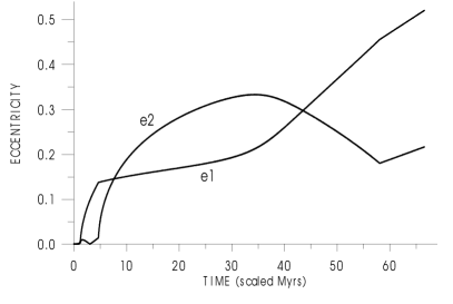
Figure 2: Eccentricities evolution after capture in the 2/1 resonance

3 Evolution under Capture

We now introduce our third body $m_{2}$ in the system, with an initial orbit exterior to $m_{1}$. We assume that $m_{2}$ does not have a tidal interaction with $m_{0}$ and that its orbit around $m_{0}$ is only perturbed by the gravitational interaction with $m_{1}$. When the semimajor axis of $m_{1}$ increases, mean-motion resonances between both satellites are reached. Capture then can take place. We performed a series of numerical simulations of the trapping process (and posterior orbital evolution within the resonance). The masses and initial conditions used in the simulation shown in this section were given by the following parameters:

$$\begin{array}[]{l@{\hspace{1cm}}l}m_{1}=4.684\times 10^{-5}m_{0}\hfil\hskip 28.45274pt&m_{2}=2.523\times 10^{-5}m_{0}\\ a_{1(0)}=5.76R_{0}\hfil\hskip 28.45274pt&a_{2(0)}=9.40R_{0}\\ e_{1(0)}=0.0008\hfil\hskip 28.45274pt&e_{2(0)}=0.0003\\ R_{0}=7.14\times 10^{7}m\hfil\hskip 28.45274pt&\Omega=1.75\times 10^{-4}s^{-1}\\ k_{2}\Delta t=3s\hfil\hskip 28.45274pt\\ G=6.67\times 10^{-11}m^{3}kg^{-1}s^{-2}.\hfil\hskip 28.45274pt\\ \end{array}$$

The masses correspond to those of Io and Europa in units of Jupiter’s mass. $R_{0}$ and $\Omega$ are the equatorial radius and the angular rotation velocity of Jupiter and $k_{2}\Delta t$ is a scaled value, approximately 400 times the actual value for Jupiter (the estimated $Q$ of Jupiter is very large, see Yoder 1979, Peale 1999). The initial semimajor axis of the outer mass, $a_{2(0)}$, corresponds to the current semimajor axis of Europa; that of $a_{1(0)}$ is a little less than the current semimajor axis of Io. The initial ratio of mean motions ($n_{1}/n_{2}$) was then 2.234. Since the satellites were placed above the synchronous orbit ($n_{1}<\Omega$), the effect of the tidal friction was to increase the orbit of Io. During the whole experiment, $a_{1}$ increases, after capture into resonance, from $5.9R_{0}$ to $9.8R_{0}$.

The system evolves with the innermost satellite receding from the planet up to the moment where the system is captured into a resonance. In the example presented in this section, the 2/1 resonance is soon reached ($t\sim 1.2$ Myr in the scaled time) and the system is trapped in this resonance. Figure 2, shows the evolution of the eccentricities after capture. It is worth noting that the variation is not nearly monotonic as seen in simplified models. The values increase and decrease following the position of the perihelia of the orbits (figure 3), a coupling that is usually not considered in many studies. The most notorious phenomenon is the elbow discontinuities at $t\sim 4.65$ and $t\sim 58$ scaled Myrs. The first elbow occurs when the two orbits cease having parallel semimajor axes and the second elbow corresponds to a return to parallelism after a long evolution through stationary solutions with non-aligned apses. In another event, which occurs at $t\sim 3.05$ scaled Myrs, the eccentricity of the inner satellite becomes close to zero and the alignment of the semimajor axes change from anti-parallel to parallel. (From $\Delta\varpi=180^{\circ}$ to $\Delta\varpi=0^{\circ}$.) The several phases of the evolution in low eccentricities may be compared to the phase portraits of 2/1-resonant planetary systems, given by Callegari et al. (2003). The mode III of Callegari et al has a similar behavior showing stationary solutions changing from $\Delta\varpi=180^{\circ}$ to $\Delta\varpi=0^{\circ}$ when a given energy level is crossed.

It is worth noting that this behavior is not reported in the literature, even in complex models such as those studied by Gomes (1998) and Murray et al. (2002). We can only assume that their simulations were not extended for a long enough time to allow these late stages of the evolution of the system to appear.

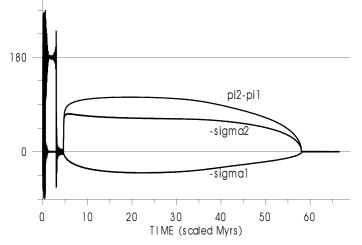
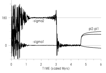
Figure 3: Top: Evolution of the angles $\Delta\varpi=(\varpi_{2}-\varpi_{1})$, $-\sigma_{1}=\lambda_{1}-2\lambda_{2}+\varpi_{1}$ and $-\sigma_{2}=\lambda_{1}-2\lambda_{2}+\varpi_{2}$ after trapping in the 2/1 resonance. Bottom: Enlargement of the initial part.

Comparing these results with the observed configuration of real bodies, we note that the current orbits of Io and Europa have anti-aligned periapses as those of the given example before $t\sim 3.05$. We stress, however, that the time scale of our experiment cannot be compared with that of the real satellite system, for several reasons. The most important is that our simulations started at a time when the bodies were already at the brink of the resonance. Of a lesser importance, but significant enough to keep in mind if the real Io-Europa pair is meant, is that the adopted time scale flows at least 400 times faster than the real one. Additionally, in the actual Galilean system, the Laplacian resonance has prevented the Io-Europa subsystem from reaching the deeper libration zone of the 2/1 resonance. Thus, it is unlikely that these satellites will ever display such turnabouts in libration, even in the far future. For extrasolar planetary systems, the current orbits of the two planets orbiting the star Gliese 876 are close to have aligned periapses as shown in the above simulations between $t\sim 3.05$ and $t\sim 4.65$. According to Lee and Peale (2002, 2003), this system may have evolved during a certain time in interaction with a remnant dust disk, but the evolution stopped when the disk dissipated. As shown by Beaugé et al. (2003), the actual orbital parameters of this system are somewhat different of those corresponding to an exact resonant stationary solution with aligned periapses. We may expect that the accumulation of precise observations may give slightly different orbital elements or, a second possibility, confirm that the periapses are not actually aligned but oscillating about the exact alignment.

From the dynamical point of view, the more striking behavior is that appearing in the interval between $t\sim 4.65$ and $t\sim 58$ scaled Myrs. During this time, the system passes through a sequence of stationary solutions in which the two periapses are fixed one with respect to another. However, $\Delta\varpi$ is no longer $0^{o}$ or $180^{o}$ as before. In the beginning of this interval, $\Delta\varpi$ increases very fast from $0^{o}$ to about $80^{o}$, then, it continues increasing up to $100-110^{o}$ and, thereafter, decreases slowly to zero again. These stationary solutions show asymmetric librations of the angles $\sigma_{1}$ and $\sigma_{2}$, a phenomenon until recently only known in the restricted asteroidal case (Beaugé 1994, Jancart et al. 2002). For illustration purposes, figure 4 shows, on the right side, planetary orbits in the case of an asymmetric stationary solution where the periapses $\Pi_{1}$ and $\Pi_{2}$ are separated by $84^{o}$. That figure also shows, on the left side, a symmetric stationary solution with the same eccentricities (no matter if not stable). In the symmetric stationary solution with aligned periapses, we have $\sigma_{1}=\sigma_{2}=0$, meaning that, not only the two periapses are aligned, but the planets have symmetric pericentric conjunctions in which both masses pass by the periapses, simultaneously, once at each synodic period. The distance of the planets, at the symmetric conjunctions, is $a_{2}(1-e_{2})-a_{1}(1-e_{1})$, a value that decreases rapidly as $e_{2}$ grows. In the asymmetric stationary solutions, the periapses shift away one from another and the conjunctions take place at an intermediate position. This asymmetry allows the quantity $a_{2}(1-e_{2})-a_{1}(1-e_{1})$ to approach zero, and even change sign, without necessarily leading to an actual collision. Nevertheless, since conjunction may occur at places where both planets come very close to each other, we cannot expect that the solutions continue to be stable for very large masses. Beaugé et al. (2003) have shown that these orbits may only exist for planet masses less than $\sim 10^{-2}$ of the central body.

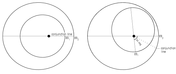
Figure 4: Left: Symmetric stationary solution with aligned periapses. Right: Asymmetric stationary solution with $|\Delta\varpi|=84^{\circ}$. The periapses are the points $\Pi_{1}$ and $\Pi_{2}$. The eccentricities are $e_{1}=0.286$ and $e_{2}=0.3$.

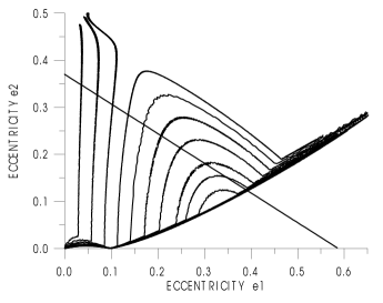
Figure 5: Families of stationary solutions of the 2/1 resonance shown in the plane $(e_{1},e_{2})$. Inner mass is $\,m_{1}=4.5\times 10^{-5}$. Each curve represents a different value of $m_{2}$; From left to right $m_{2}=0.5,1.0,1.5,2.0,2.5,3.0,3.5,4.0,4.25,4.5\times 10^{-5}$. The lines corresponding to $m_{2}=4.75,5.0,5.25\times 10^{-5}$ accumulate at the bottom of the set. This accumulation marks the separation between the region of asymmetric stationary solutions (above) and symmetrical ones (on and below). The diagonal straight line across the figure indicates the limit above which the two orbits necessarily intersect.

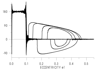
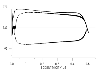
Figure 6: Values of $\Delta\varpi$ for the families of stationary solutions shown in figure 5. Top: $m_{2}\geq 2.0\times 10^{-5}$: the asymmetric solutions bifurcate from $\Delta\varpi=180^{o}$. For $m_{2}\geq 5.0\times 10^{-5}$ no asymmetry appears and $\Delta\varpi$ does not bifurcate. Bottom: $m_{2}\leq 1.5\times 10^{-5}$: the asymmetric solutions bifurcate from $\Delta\varpi=180^{o}$.

4 Asymmetric Stationary Solutions

In the restricted asteroidal problem, it is known that asymmetric solutions only exist in the exterior case, that is, when the asteroid is moving in an orbit exterior to the planet orbit. Even then, these solutions are only detected in resonances of the type $p/1$, being 2/1 and 3/1 the most important ones (Beaugé 1994). In this section, we search for analogous asymmetric solutions in the case of two finite masses, and study their dependence with $m_{1}/m_{2}$. In particular, we are interested in detecting the minimum value of the mass ratio for which these solutions are still present. According to Hadjidemetriou (2002), symmetric periodic orbits in the planetary 2/1 resonance are only stable for values of $m_{1}/m_{2}<1$. We will see that asymmetric solutions allow for a larger range of masses.

In these experiments, $k_{2}\Delta t$ was increased to 15 s, a value 5 times larger than that used in the experiment discussed in previous section. This was a limit choice for this parameter; indeed, we can see small fluctuations in some of the lines indicating that the variations were not adiabatic enough to keep the solutions stationary, forcing small oscillations about the stationary solution.

4.1 2/1 Resonance

For this commensurability, the mass $m_{1}$ of the inner orbiting body was fixed at $4.5\times 10^{-5}$ and the outer mass $m_{2}$ was varied in the range $0.5-5.25\times 10^{-5}$. The results are shown in figures 5 and 6.

Figure 5 shows that asymmetric stationary solutions exist for all values of $m_{1}/m_{2}$ above a limit close to 1 ($m_{1}/m_{2}>\sim 0.97$). As the ratio $m_{1}/m_{2}$ decreases approaching this limit, the interval of eccentricities where asymmetric solutions exist decreases to zero. For almost all mass-ratios within this range, asymmetric stationary solutions in which the two orbits cross one another exist. The inclined straight line in figure 5 shows the values of $e_{1}$ and $e_{2}$ such that the apocentric distance of $m_{1}$ equals the pericentric distance of $m_{2}$. For all initial conditions above this curve, the two orbits may intersect.

The equilibrium values of $\Delta\varpi$ are shown in figure 6. In the evolution paths with $m_{2}\geq 2.0\times 10^{-5}$, the asymmetric solutions bifurcate from symmetric solutions with aligned periapses; at variance, for $m_{2}\leq 1.5\times 10^{-5}$, the asymmetric solutions bifurcate from low-eccentricity symmetric solutions with anti-aligned periapses. The two situations are shown in separate figures also because, for $m_{2}\leq 1.5\times 10^{-5}$, the eccentricity $e_{1}$ has only a very small variation, while the $e_{2}$ has a large variation and thus the variations are more clear shown if it lies in the horizontal axis.

It is worth comparing these results on the 2/1 resonance with the periodic orbits of Hadjidemetriou (2002). His conclusion that stable solutions are only found with $m_{1}/m_{2}<1$ is true only if we restrict the domain to large eccentricity symmetric orbits. In the general case, stable stationary solutions can be found for much higher values of the mass ratio.

One last point to mention is that the asymmetric solutions appear as a bifurcation point where symmetric solutions change from stable to unstable. This bifurcation generates two distinct families of asymmetric solutions, each independent of the other. When a trapping occurs, the system may be captured in either one or the other of the two new centers. This is clearly seen in figures 6 where approximately half of the solutions departed in one direction and half in the opposite one.

4.2 3/1 Resonance

In the restricted asteroidal problem, asymmetric solutions exist for all exterior resonances of the type $p/1$ (i.e. 2/1, 3/1, 4/1, etc.). A series of simulations was then done to see whether the general three-body problem also presented asymmetric points in the 3/1 resonance. As in the previous subsection the relative mass of the innermost orbiting body was fixed at $4.5\times 10^{-5}$ and the outer value was varied from $2.5\times 10^{-5}$ to $5.5\times 10^{-5}$ in steps of $0.5\times 10^{-5}$. The remaining parameters were chosen as:

$$\begin{array}[]{l@{\hspace{2cm}}l}a_{1(0)}=5.85R_{0}\hfil\hskip 56.9055pt&a_{2(0)}=12.4R_{0}\\ e_{1(0)}=0.0010\hfil\hskip 56.9055pt&e_{2(0)}=0.0004\\ \end{array}$$

The results are shown in figs. 7 and 8. The capture into resonance occurs quickly and $\Delta\varpi$ reaches $180^{o}$ remaining there up to the bifurcation and switching to an asymmetric stationary solution. Periodic orbits with aligned periapses were not seen, although, in the very beginning of the simulations $\Delta\varpi$ appeared temporarily oscillating about $0^{o}$ with a large amplitude. The more characteristic feature of the 3/1-resonant asymmetric stationary solutions is the boundary between symmetric and asymmetric regions at $e_{2}\sim 0.11$ (elbows line in figure 7). In this resonance, asymmetric stationary solutions exist for all values of the mass ratio (greater or smaller than unity) up to the limit corresponding to a curve whose elbows occurs for $e_{1}\sim 1$. For mass ratios larger than this, the stationary solution lines will remain below the $e_{2}\sim 0.11$ limit for all $e_{1}<1$.

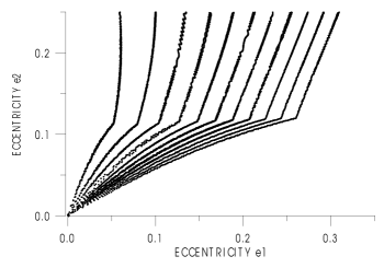
Figure 7: Families of stationary solutions of the 3/1 resonance shown in the plane $e_{1},e_{2}$; $\,m_{1}=4.5\times 10^{-5}$; from left to right $m_{2}=0.5,1.0,1,5,2.0,2.5,3.0,3.5,4.0,4.5,5.0,5.5\times 10^{-5}$. The line formed by the elbows of the curves, at $e_{2}\sim 0.11$, separates the symmetric (below) and asymmetric (above) stationary solutions.

Figure 8: Values of $\Delta\varpi$ for the families of stationary solutions shown in figure 7 for which $m_{2}\geq 2.5\times 10^{-5}$; In the 3/1 resonance the asymmetric solutions bifurcate from symmetric solutions with anti-aligned periapses ($\Delta\varpi=180^{o}$)

5 Conclusions

In this paper, we presented a series of numerical simulations of the evolution of systems of two massive orbiting bodies after capture into the 2/1 and 3/1 resonances. Albeit with a change in the timescale of the solutions, the same behavior can represent the evolution of a pair of satellites around one planet (the data used were those from the Io-Europa pair) or two exoplanets orbiting close to a star. The simulations were done using tides in the central body as the source of the non-conservative perturbation, but the results do not depend on the particular force used, and should happen in similar way with other non-conservative forces provided its effects are sufficiently slow to have adiabatic variations. Thus, the same behavior is expected to hold in the evolution of exoplanets captured into a 2/1 or 3/1 resonance due to (for example) interactions with a residual disk of matter or any other non-conservative force. For instance, Lee and Peale (2003) have obtained results very similar to those discussed in section 3 in a simulation of a system of 2 planets in which the outer planet is driven inward by torques exerted on it by outside nebular material.

Finally, we have shown that the evolution of resonant trapped massive bodies is not simple. Our results show a surprising richness of solutions: symmetric librations around $\Delta\varpi=0$ and around $\Delta\varpi=\pi$, asymmetric solutions with a wide range of values of $\Delta\varpi$, turnabouts from one configuration to another during the secular variation of semimajor axes, etc. Many of these solutions exist for large values of the eccentricities. As our knowledge of extrasolar planets continues to grow, it will be interesting to see how many of these possible configurations actually occur in the real world.

Acknowledgements

The authors acknowledge the support of FAPESP and CNPq to this investigation and the Instituto de Pesquisas Espaciais, INPE, where C.Beaugé was visiting investigator during the realization of this investigation. The research subject “Interplay of Tides and Resonances” was suggested to SFM by Iwan Williams.

References

- [1] Aksnes, K. and Franklin, F.A.: 2001, “Secular Acceleration of Io derived from Mutual Satellite Events”, Astron. J. 122, 2734-2739.
- [2] Beaugé, C.: 1994, “Asymmetric Librations in Exterior Resonances”, Cel. Mech. Dyn. Astron. 60, 225-248.
- [3] Beaugé, C., Ferraz-Mello, S. and Michtchenko, T.A.: 2003, “Extrasolar Planets in Mean-Morion Resonance: Apsidal and Asymmetric Stationary Solutions”, Astroph. J., submitted.
- [4] Callegari, Jr., N., Michtchenko, T.A. and Ferraz-Mello, S.: 2003, “Dynamics of two planets in the 2:1 and 3:2 mean-motion resonances” (in preparation).
- [5] Ferraz-Mello, S.: 1979, Dynamics of the Galilean Satellites, IAG-USP, São Paulo.
- [6] Ferraz-Mello, S.: 1987, “Averaging the Elliptic Asteroidal Problem Near a First-Order Resonance”. Astron. J. 94, 208-212.
- [7] Gomes, R. S.: 1998: “Orbital Evolution in Resonance Lock. II. Two Mutually Perturbing Bodies”, Astron. J. 116, 997-1005.
- [8] Hadjidemetriou, J.D.: 2002, “Resonant Periodic Motion and the Stability of the Extrasolar Planetary Systems” Celest. Mech. Dyn. Astron. 83, 141-154.
- [9] Jancart, S.: 2002, Résonances et Dissipations, Dr. Thesis, Presses Universitaires, Namur.
- [10] Jancart, S., Lemaitre, A., and Istace, A.: 2002, “Second Fundamental Model of Resonance with Asymmetric Equilibria” Celest. Mech. Dyn. Astron. 84, 197-221.
- [11] Lee, M.H. and Peale, S.J.: 2002, “Dynamics and Origin of the 2:1 Orbital Resonances of the GJ 876 Planets” Astroph. J. 567, 596-609.
- [12] Lee, M.H. and Peale, S.J.: 2003, “Extrasolar Planets and Mean-Motion Resonances” ASP Conf. Series (in press).
- [13] Lieske, J.H.: 1987, “Galilean Satellites Evolution - Observational Evidence for Secular Changes in Mean-Motions” Astron. Astrophys. 176, 146-158.
- [14] Lieske, J.H.: 1998, “Galilean Satellites Ephemerides E5”, Astron. Astrophys. Supp. Ser. 129, 205-217.
- [15] MacDonald, G.J.F.: 1964, “Tidal Friction” Rev.Geophys. 2, 467-541.
- [16] Mignard, F.: 1981, “The Evolution of the Lunar Orbit Revisited. I”, Moon and Planets, 20, 301-315.
- [17] Murray, N., Paskowitz, M. and Holman, M.: 2002, “Eccentricity Evolution of Resonant Migrating Planets”, Astroph. J. 565, 608-620.
- [18] Peale, S.J.: 1999, “Origin and Evolution of the Natural Satellites” Ann. Rev. Astron. Astroph. 37, 533-602.
- [19] Tisserand, F.: 1896, Traité de Mécanique Céleste, Gauthier-Villars, Paris, vol. IV.
- [20] Touma, J. and Wisdom, J.: 1994, “Evolution of the Earth-Moon System”, Astron. J. 108, 1943-1961.
- [21] Wu, Y. and Goldreich, P.: 2002, “Tidal Evolution of the Planetary System around HD 83443”, Astroph. J. 564, 1024-1027.
- [22] Yoder, C.F.: 1979, “How tidal heating in Io drives the Galilean Orbital Resonance Locks”,Nature 279, 767-770.