Echo Tomography of Black Hole Accretion Flows a

Abstract

We discuss technologies for micro-arcsec echo mapping of black hole accretion flows in Active Galactic Nuclei (AGN). Echo mapping employs time delays, Doppler shifts, and photoionisation physics to map the geometry, kinematics, and physical conditions in the reprocessing region close to a compact time-variable source of ionizing radiation. Time delay maps are derived from detailed analysis of variations in lightcurves at different wavelengths. Echo mapping is a maturing technology at a stage of development similar to that of radio interferometry just before the VLA. The first important results are in, confirming the basic assumptions of the method, measuring the sizes of AGN emission line regions, delivering dozens of black hole masses, and showing the promise of the technique. Resolution limits with existing AGN monitoring datasets are typically $\sim$5-10 light days. This should improve down to 1-2 light days in the next-generation echo mapping experiments, using facilities like Kronos and Robonet that are designed for and dedicated to sustained spectroscopic monitoring. A light day is 0.4 micro-arcsec at a redshift of 0.1, thus echo mapping probes regions $10^{3}$ times smaller than VLBI, and $10^{5}$ times smaller than HST.

1 Micro-Arcsec Echo Tomography

Angular resolution is a discovery frontier that drives the development of astronomical technology. HST delighted the public and transformed astronomy by delivering stunning sub-arcsec images at ultraviolet, optical, and more recently infrared wavelengths. Large ground-based telescopes can now produce sub-arcsec images at infrared wavelengths by using adaptive optics to compensate for atmospheric turbulence. Sub-arcsec radio maps are routinely constructed from complex visibility measurements obtained with multi-element radio interferometers (VLA, Merlin), and milli-arcsec resolution is achieved with the Very Long Baseline Array (VLBA). The most ambitious technology on the angular resolution horizon is the Micro-Arcsec X-ray Interferometry Mission, MAXIM, which may one day image the flow of material into nearby black hole event horizons.

Today we are already exploring the micro-arcsec structure of black hole accretion flows through echo tomography experiments. Tomography is an indirect imaging technique that recovers an image from measurements of projections of that image. Tomography is analogous to interferometry, except that the measurements are of projections rather than fourier components of the image. Echo mapping employs time-resolved spectrophotometry to record spectral variations in which detailed information on spatial and kinematic structure is coded as time delays and Doppler shifts. This article discusses echo tomography technologies in use and under development for micro-arcsec mapping of black hole accretion flows.

1.1 Black Hole Accretion Flows

Black holes come in two varieties: stellar-mass holes ($M\sim 10M_{\odot}$) in X-ray binaries, and supermassive black holes ($M\sim 10^{6-9}M_{\odot}$) in the nuclei of galaxies. Accretion disks convey angular momentum outward as matter spirals inward to feed the central black hole. Accretion theory and black hole scaling laws can be tested by comparing phenomena in X-ray binaries and active galactic nuclei (AGN). Although they are too small for direct or interferometric imaging, these accretion flows can be resolved by echo tomography.

Current models of AGN spectral energy distributions include optical to X-ray emission from the accretion disk, infrared emission from a dusty molecular torus encircling and from some viewing angles obscuring the disk, and relativistically beamed radio to X-ray emission from jets. Emission lines arise from reprocessing of X-ray and EUV radiation in two kinematically-distinct regions, the broad line region (BLR) with $V\sim 10^{4}~{}{\rm km\ s}^{-1}$, and the narrow-line region (NLR) with $V<10^{3}~{}{\rm km\ s}^{-1}$. The NLR, resolved by HST, has a bi-polar morphology interpreted as wide cones of ionising radiation emerging from the unresolved nucleus. The accretion disk and BLR are unresolved, but these regions vary on timescales of days to months in response to erratic changes in ionising radiation from regions still closer to the black hole. Light travel time within the system produces observable time delays, providing indirect information on the size and structure of the disk and BLR, which make these regions accessible to echo tomography.

1.2 Time Delay Paraboloids

Figure 1: Ionizing photons from a compact source are reprocessed by gas clouds in a thin spherical shell. A distant observer sees the reprocessed photons arrive with a time delay ranging from 0 for reprocessing at the near edge of the shell to $2R/c$ for reprocessing at the far edge. The iso-delay paraboloids slice the shell into zones with areas proportional to the range of delays.

Reverberation mapping [1] relies on a compact erratically variable source of ionizing radiation embedded within the region that we wish to probe. Heated and photoionised gas reprocesses the ionizing radiation into ultraviolet, optical and infrared continuum and line emission. Variations in the central source launch spherical waves of heating and ionization that expand at the speed of light through the surrounding gas. Each change in ionization triggers a corresponding change in the reprocessed emission. In AGNs, the reprocessing time (hours) is small compared with light travel time (days), so that the delay seen by a distant observer is dominated by the light travel time.

The iso-delay surfaces are ellipsoids with one focus at the central source and the other at the observer, and are well approximated by paraboloids in the reprocessing region near the central source (Fig. 1). The time delay is

$$\tau=\frac{R}{c}(1+\cos{\theta})\ ,$$ (1)

for a reprocessing site at a radius $R$ from the nucleus and azimuth $\theta$, measured from 0 on the far side of the nucleus to $180^{\circ}$ on the line of sight between the nucleus and the observer. The delay is 0 for gas on the line of sight between us and the nucleus, and $2R/c$ for gas directly behind the nucleus (Fig. 1). The time delay map, $\Psi(\tau)$, is a 1-dimensional map of the emission line region, effectively slicing up the region along the nested set of iso-delay paraboloids.

1.3 The Driving Lightcurve

The ionizing radiation that drives reprocessing includes EUV photons that are strongly absorbed by neutral hydrogen in the interstellar medium, and are therefore not directly observable. Fortunately, we see nearly co-temporal variations in continuum lightcurves at most ultraviolet and optical wavelengths, suggesting that the continuum forms in a region much smaller than the emission line regions. The continuum light curve $f_{c}(t)$ thus serves as a useful surrogate for the unobservable light curve of the ionizing radiation.

1.4 Linear and Linerized Reverberation Models

In the simplest linear reverberation model, reprocessing sites span a range of time delays, and the line light curve $f_{\ell}(t)$ is a weighted sum of time-delayed copies of the continuum light curve $f_{c}(t)$,

$$f_{\ell}(t)=\int_{0}^{\infty}\Psi_{\ell}(\tau)\ f_{c}(t-\tau)\ d\tau.$$ (2)

In this convolution integral, $\Psi_{\ell}(\tau)$ is the “transfer function”, or “convolution kernel”, or “delay map” of the emission line $\ell$. This describes the strength of the reprocessed emission that arises from the regions between pairs of iso-delay paraboloids. Of course each emission line has its own time variations $f_{\ell}(t)$ and corresponding delay map $\Psi_{\ell}(\tau)$.

Echo mapping aims to recover $\Psi_{\ell}(\tau)$ from measurements of $f_{\ell}(t)$ and $f_{c}(t)$ made at specific times $t_{i}$. To fit such observations, the model above is too simple in several respects. First, additional sources of light contribute to the observed continuum and emission-line fluxes. Examples are background starlight, and narrow emission lines. Since these sources do not vary on the reverberation timescale, they simply add constants to $f_{\ell}(t)$ and $f_{c}(t)$,

$$f_{\ell}(t)=f_{\ell}^{B}+\int_{0}^{\infty}\Psi_{\ell}(\tau)\ \left[f_{c}(t-\tau)-f_{c}^{B}\right]d\tau.$$ (3)

This linearized model also useful as a tangent line approximation to a non-linear line response. The “background” fluxes, $f_{\ell}^{B}$ for the line and $f_{c}^{B}$ for the continuum, are set somewhere near the middle of the range of values spanned by the observations. The delay map $\Psi_{\ell}(\tau)$ then gives the marginal response of the line emission from gas at time delay $\tau$, to changes in ionising radiation above or below the chosen background level.

1.5 Inversion Methods

Three practical methods have been developed for deriving $\Psi_{\ell}(\tau)$ from observations. The Regularized Linear Inversion (RLI) method [2, 3] and the Subtractive Optimally-Localized Averages (SOLA) method [4], use the linear reprocessing model to directly invert well-sampled equally-spaced or interpolated lightcurves. The Maximum Entropy Method (MEM), is useful for the more sophisticated fitting problems, allowing for non-uniform sampling and data quality in the lightcurves, and non-linear reprocessing models. The echo mapping results presented in this paper are obtained with the maximum entropy echo mapping code MEMECHO [5, 6], which makes use of the maximum entropy fitting code MEMSYS [7].

2 First-Generation Echo Mapping Experiments

2.1 Size and Radial Structure

To illustrate the quality of the echo maps constructed from current datasets, Fig. 2 shows a MEMECHO fit of the linearized echo model of Eqn. (3) to H$\beta$  and optical continuum lightcurves of NGC 5548 [5]. The lightcurves are extracted from optical spectra arising from the 9-month AGN Watch campaign in 1989. Data from many observatories are inter-calibrated, and the error bars are estimated from the internal consistency of independent measurements made close together in time. Subtracting the continuum background $f_{c}^{B}$, convolving with the delay map $\Psi_{\ell}(\tau)$, and adding the line background $f_{\ell}^{B}$, gives the H$\beta$  light curve. The three fits shown, all with $\chi^{2}/N=1$, give some impression of the uncertainty in the fit arising from the noise level of the data and gaps in time coverage.

Figure 2: Echo maps of H$\beta$  emission in NGC 5548 recovered by fitting to data from a 9-month AGN Watch monitoring campaign in 1989. The optical continuum light curve (lower panel) is convolved with the delay map (top left) to produce the H$\beta$  emission-line light curve (top right). Horizontal dashed lines give the mean line and continuum fluxes. Three fits are shown to indicate likely uncertainties. Data from (Ref. [5]).

The delay map of H$\beta$  emission in NGC 5548 rises to a peak at 20 days, and declines to low values by 40 days. This measures the size of the H$\beta$  emission-line region, $\sim 20$ light days. Tests with simulated data using the same time sampling and signal-to-noise ratios indicates that the resolution achieved in this map is about 10 days. Similar maps for a variety of ultraviolet emission lines indicate that high ionisation lines have smaller delays than low-ionisation lines [8]. This implies that reprocessing occurs over a wide range of radii, with higher ionisation closer to the nucleus.

2.2 Velocity-Delay Maps

To derive a Doppler-delay map from observations, simply slice the observed spectra into wavelength bins, and recover a delay map from the light curve at each wavelength. This is a simple extension of the echo model used to fit continuum and emission-line lightcurves. At each wavelength $\lambda$ and time $t$, obtain the emission-line flux

$$f_{\ell}(v,t)=f_{\ell}^{B}(v)+\int_{0}^{\infty}\left[f_{c}(t-\tau)-f_{c}^{B}\right]\ \Psi_{\ell}(v,\tau)\ d\tau$$ (4)

by adding time-delayed copies of the continuum light curve to a time-independent background spectrum $f_{\ell}^{B}(v)$.

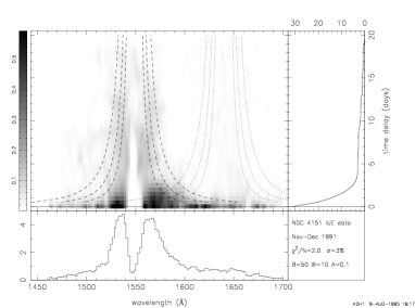
Figure 3: Velocity-delay map of C iv  1550 emission (and blended He ii  1640 emission) in NGC 4151 recovered by fitting to 44 IUE spectra. Absorption wipes out the core of the C iv  line. Dashed curves give escape velocity envelopes for masses 0.5, 1.0, and $2.0\times 10^{7}$M_⊙. An inverse correlation between velocity width and time delay supports the hypothesis of virial motions, and yields virial mass estimates for dozens of supermassive black holes. Black hole masses estimated from the H$\beta$  emission line, based on cross-correlation time delay and FWHM of the line in the variable component of the light, are from (Ref. [9]).

In Fig. 3, the velocity-delay map for C iv  1550 and He ii  1640 emission was reconstructed from 44 IUE spectra of NGC 4151 [10]. While spanning only 36 days, this campaign recorded favorable continuum variations, including a bumpy exponential decline followed by a rapid rise, which were sufficient to support echo mapping on delays from 0 to 20 days. Although a strong C iv  absorption feature obliterates the delay structure at small velocities, it is clear that a wide range of velocities is present at small delays, and and smaller range at larger delays. The dashed curves in Fig. 3 give escape velocity envelopes $v=\sqrt{2GM/c\tau}$ for masses 0.5, 1.0, and $2.0\times 10^{7}$ M_⊙. This clearly supports the hypothesis of virial motions, and suggests a mass of order $10^{7}$ M_⊙.

2.3 Black Hole Masses

With the assumption of virial motions, black hole mass can be estimated from

$$M=f\frac{c\ \tau\ \sigma^{2}}{G}\ ,$$ (5)

where $\tau$ and $\sigma$ are the time delay and velocity dispersion of an emission line, and $f$ is a form factor allowing for uncertain details of the flow geometry, kinematics and orientation. The virial hypothesis predicts that lines formed at different radii in the same object should obey $\sigma\propto\tau^{-1/2}$. The internal consistency of mass estimates from different lines in NGC 5548 [8, 11], and in a few other objects [12], supports the virial hypothesis. An uncertainty of perhaps a factor of 3 remains due to the factor $f$ representing ambiguity in the detailed kinematics of the flow. [13]

Reverberation masses ranging from $10^{6}$ to $10^{9}$M_⊙ are now available for several dozen AGNs [9, 14] based on cross-correlation time delays and rms widths of H$\beta$ emission (Fig. 3). At present there are no reverberation masses for high-redshift AGNs. However, the low-redshift reverberation masses serve to calibrate an empirical mass-radius-luminosity relationship from which black hole masses may be estimated for more distant systems [9, 14]. This extends black hole mass estimates to all AGN with a measured H$\beta$  line width. Such estimates are useful in the investigation of the evolution of black hole masses and accretion rates.

2.4 Temperature Profiles of AGN Accretion Disks

In theory, steady-state accretion disks have a $T\propto(M\dot{M})^{1/4}R^{-3/4}$ structure, and give rise to a characteristic spectrum $f_{\nu}\propto(M\dot{M})^{2/3}\lambda^{-1/3}D^{-2}$. Here $\dot{M}$ is the accretion rate and $D$ is the distance. AGN spectra are generally much redder than this, casting doubt on the validity of the disk model. We can measure the $T(R)$ profiles of AGN accretion disks by measuring $\lambda$-dependent continuum reverberations arising from the disk surface. With $T(R)$ decreasing outwards, reverberations at smaller $R$ and shorter $\lambda$ will preceed those at larger $R$ and longer $\lambda$. Time delays increase as $\tau\approx R/c$, and blackbody spectra peak at $T\approx hc/k\lambda$, so that shorter wavelengths sense disk annuli at higher temperatures. A disk surface with $T\propto R^{-b}$ will reverberates with a delay spectrum $\tau\propto\lambda^{-1/b}$. The $T\propto(M\dot{M})^{1/4}R^{-3/4}$ profile of a steady-state disk corresponds to $\tau\propto(M\dot{M})^{1/3}\lambda^{4/3}$.

AGN continuum lightcurves at different wavelengths exhibit a high degree of correlation, with time delays generally shorter than a few days. In the best-observed case [15], NGC 7489, the time delay does increase with wavelength, consistent with $\tau\propto\lambda^{4/3}$. Moreover, subtracting bright and faint spectra yields a difference spectrum close to $f_{\nu}\propto\lambda^{-1/3}$. These results suggest that variability may be an effective way to isolate the disk component of AGN spectra. The NGC 7489 results yield estimates for $M\dot{M}$ and $D$, leading to an encouragingly sensible estimate of the Hubble constant, $H_{0}\sqrt{\cos{i}}\approx 42\pm 9$km s^-1/Mpc. If similar results are obtained for a larger sample of AGNs, spanning a range of redshifts, the results may be used to to probe cosmology beyond the redshift horizon of supernovae.

2.5 Highlights of First-Generation Echo Mapping Experiments

The first decade of echo mapping experiments, a series of intensive monitoring campaigns undertaken in particular by the AGN Watch consortium (http://www.astronomy.ohio-state.edu/~agnwatch/), has sharpened our knowledge of AGNs in numerous ways. The basic photoionisation picture is well supported by the correlated emission line and continuum variations, with lines lagging behind the continuum, in several dozen nearby AGNs. Interpreting the time delay, $\tau$, as light travel time, the inferred BLR sizes, $R\sim c\tau$, are 10-100 times smaller than expected from earlier single-cloud photoionization models. The smaller size implies higher densities, $n\sim 10^{11}{\rm cm}^{-3}$. Higher-ionization lines have smaller delays and larger widths [16], suggesting a radially-stratified ionization structure with virial kinematics[11]. Larger time delays in more luminous sources imply $R\propto L^{0.5-0.7}$, compatible with an ionization-bounded BLR [14]. In several sources, an anti-correlation between velocity dispersions and time delays is consistent with virial motions. [8, 11, 12] On this basis, “reverberation masses” are available for black holes in AGNs for which the H$\beta$  velocity dispersion $\sigma$ and time delays $\tau$ are measured. This in turn calibrates an empirical $M$–$\sigma$–$L$ relationship from which black hole masses can be estimated for all AGNs with measured H$\beta$  line widths [9]. We thus have a foundation for demographic studies of the growth of supermassive black holes over cosmic time.

3 Next-Generation Echo Mapping Experiments

In the next decade, striking improvements in echo mapping capabilities are expected from technology developments on two fronts.

First, improvements in the quality and time sampling of spectrophotometric monitoring datasets should dramatically improve the resolution and fidelity of the maps. The present 5-10 day resolution of echo maps is limited by the noise levels (typically 3%), cadence, and duration of the lightcurves. Just as the VLA dramatically improved the $U-V$ coverage and hence resolution and fidelity of radio maps, so the echo maps will be greatly improved by using facilities that are specifically designed for and dedicated to sustained spectrophotometric monitoring.

• RoboNet (http://star-www.st-and.ac.uk/~kdh1/jifpage.html) is a global network of 2-m robotic telescopes equipped with identical multi-band CCD imagers and integral-field unit spectrographs.

• Queue-scheduled spectrographs on large ground-based telescopes are ideal for sustained daily monitoring, and will enable echo mapping of fainter AGNs at larger redshifts.

• Kronos (http://www.astronomy.ohio-state.edu/~kronos) is a small space telescope (NASA MidEx) equipped with simultaneous X-ray, UV, and optical spectrographs in a 14 d orbit to enable nearly continuous coverage for weeks to months and daily sampling for hundreds of days.

What may we expect to achieve in the next-generation echo mapping experiments? Simulation tests, some of which are presented below, indicate that high fidelity echo maps with a resolution exceeding 1 light day will emerge from datasets with a time sampling $<1$ day, a duration $\sim 300$ days, and accuracies of $\sim 1$%.

Second, in tandem with better data, better models are needed to interpret the improved datasets. We currently extract lightcurves from observed spectra, and fit those lightcurves with a simple linear or linearised reprocessing model to construct delay maps for each line or wavelength independently of the others. This relatively model-independent approach ignores a great deal of prior information. Photoionisation models predict highly non-linear and anisotropic responses that are different for each emission line. Given the evidence supporting the photoionisation hypothesis, we should now aim to improve the echo maps by building in the additional constraints from photoionisation physics. The next-generation reverberation models, currently under development, will fit the entire reverberating spectrum, avoiding the need to extract lightcurves and de-blend lines, and build photoionisation physics into the fitting process. This approach should yield 5-dimensional maps of the geometry ($R$, $\theta$), kinematics ($V$), and physical conditions ($n$,$N$) in the photoionised gas.

We discuss and illustrate these developments below.

3.1 Better Datasets, Sharper Maps

Figure 4: Two simulations, each illustrating the recovery of a delay map (top left) from data points sampling an erratically varying continuum light curve (bottom) and the corresponding delay-smeared emission-line light curve (top right). The data points sample 400 epochs spaced by 1 day. In simulation 1 (left) the true map is $\Psi_{\ell}(\tau)\propto\tau e^{-\tau/10}$. In simulation 2 (right) the map has 5 sharp peaks at delays 5, 10, 20, 40, and 80 days. In both cases the reconstructed delay maps closely resemble the true maps.

Fig. 4 illustrates the recovery of 1-dimensional delay maps based on MEMECHO fits to simulated lightcurves. The time sampling and signal-to-noise ratios in these simulations are designed to resemble datasets that will arise routinely with next-generation spectrophotometric monitoring facilities, such as Kronos and RoboNet.

In both simulations, examine and compare the driving continuum lightcurve (bottom) with the responding line lightcurve (top right). The delayed maxima and minima indicate that the delay map has a mean delay of about 20 days. The fast variations evident in the continuum lightcurves appear to be washed out in the line lightcurves, which are much smoother, indicating that a range of delays is present. By eye, this is about all that we can safely infer. The line lightcurve in simulation 2 does exhibit more fast structure than that in simulation 1, but this structure is not cleanly correlated with the fast continuum variations. It is not obvious what this may imply about the delay structure. Evidently our eyes and brains have a rather limited ability to interpret reverberation datasets by inspection – much as is also the case for $U-V$ visibility measurements that are employed in interferometry.

When MEMECHO fits the two lightcurves in detail, however, information from all the small but significant changes recorded in the lightcurves is assembled to construct the delay map (top left). The two maps recovered by MEMECHO are quite distinct. In simulation 1 the delay map has a smooth distribution, rising to a rounded peak and then declining smoothly. In simulation 2 the delay map has 5 discrete peaks. In both cases the recovered maps closely resemble the true map. With such high quality data, the delay map is recovered with high fidelity. There is some blurring, of course, because no finite dataset can recover the map with infinite resolution. The resolution achieved is about 1 light day.

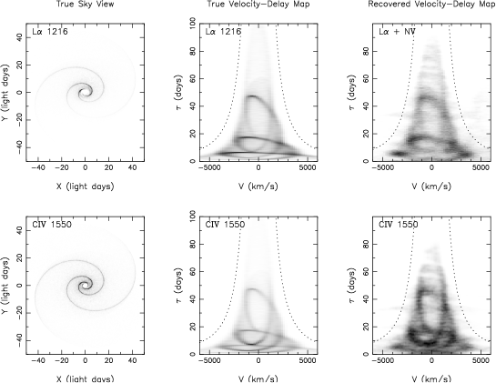
Figure 5: High-fidelity velocity-delay maps of Ly$\alpha$  and C iv  emission reconstructed from a simulated Kronos dataset spanning 200 days. The emission is assumed to arise from a Keplerian accretion disk with a two-armed trailing spiral density wave pattern (left). The spiral waves are clearly visible in the true velocity-delay map (middle) and in the map recovered from the simulated Kronos spectra (right). Dashed curves give the maximum time delay allowed at each velocity for bound gas around a black hole of mass $3\times 10^{7}$M_⊙.

Fig. 5 examines MEMECHO reconstructions of 2-dimensional velocity-delay maps from simulated Kronos datasets. This simulation illustrates the extent to which fine-scale structure in the geometry and kinematics of an AGN emission line region can be recovered from a Kronos dataset. The simulated dataset, designed to resemble a Kronos observation of NGC 5548, includes realistic noise levels allowing for the effective area curves of the Kronos spectrographs, and assuming that a 1 hour spectrum is taken every 4.8 hours for a total of 200 days. We adopt the power-law model of Kaspi & Netzer [17], in which the density $n$ and column density $N$ are power-law functions of radius, and the photoionisation code ION is used to evaluate the anisotropic and non-linear responses of the emission lines at each level of ionising continuum flux. For the geometry and kinematics we adopt a Keplerian disk with a 2-armed trailing spiral density wave. The disk is comprised of a large number of discrete clouds orbiting a black hole of mass $3\times 10^{7}$M_⊙. The co-planar Keplerian orbits are elliptical, so that each cloud spends more time near apbothron than peribothron, and are rotated by an angle proportional to the logarithm of their semi-major axes, thereby producing the spiral density wave. From the synthesized spectra, we fit continua, extract line lightcurves at each velocity, and use MEMECHO to construct velocity-delay maps for each line.

In Fig. 5, the spiral waves clearly visible on the sky view (left panel) extend out to $\approx 10^{-4}$ arcsec (the redshift of NGC 5548 is $z=0.016$). This structure is beyond the reach of foreseeable developments in direct or interferometric imaging technology. Yet the velocity-delay map (middle panel) clearly shows this spiral wave structure, and it is also clearly recognizable in the reconstructed velocity-delay map (right panel) recovered from the simulated Kronos dataset.

These results are typical of many other simulations that we have run, for a wide variety of source structures, indicating that major advances in the fidelity and information content of echo maps will arise when the data quality is significantly improved. The simulations indicate that we can sharpen our vision by a factor of 10 compared to the 5-10 day resolution that has been achieved to date.

3.2 5-Dimensional Maps: $\Psi(R,\theta,n,N,v)$

In parallel with improvements in the reverberation datasets, we must improve the models that we use to interpret the data. A great deal of information on the geometry, kinematics, and physical conditions of black hole accretion flows is encoded in the detailed reverberations of emission-line spectra. We cannot extract this information by inspection of the data. To tap this information, and reconstruct maps of black hole environments, we must aim to fit the observed reverberations in far greater detail than has previously been attempted. The next-generation echo-mapping codes, building in constraints from photoionisation physics, are currently under development. We sketch the new methods, and then illustrate some preliminary results below.

Rather than extracting line and continuum lightcurves, we now synthesize and fit $f_{\nu}(\lambda,t)$, the complete spectrum at each time. This avoids sticky problems of continuum fitting and de-blending the overlapping wings of emission lines. We model the spectrum as a sum of three components: direct light from the nucleus, reprocessed light from the surrounding gas clouds, and background light:

$$f_{\nu}(\lambda,t)=f^{D}_{\nu}(\lambda,t)+f^{R}_{\nu}(\lambda,t)+f^{B}_{\nu}(\lambda)\ .$$ (6)

The background light, $f^{B}_{\nu}(\lambda)$, allows for contamination by non-variable sources, e.g. starlight from the host galaxy. The direct light from the nucleus is

$$f^{D}_{\nu}(\lambda,t)=\frac{L(t)S_{\nu}(\lambda)}{4\pi D^{2}}\ ,$$ (7)

where $D$ is the distance, $L(t)$ is the lightcurve, and $S_{\nu}(\lambda)$ is the shape of the spectrum emerging from the nucleus. The emission-line spectrum of the reprocessed light is

$$f^{R}_{\nu}(\lambda,t)=\int_{0}^{\infty}\frac{L(t-\tau)}{4\pi D^{2}}\ \Psi_{\nu}(\lambda,\tau,L(t-\tau))\ d\tau\ ,$$ (8)

arising from a non-linear transfer function given by

$$\begin{array}[]{rl}\Psi_{\nu}(\lambda,\tau,L)&=\sum_{\ell}\ \int\int\int\int 2\pi R\ dR\ \sin{\theta}\ d\theta\ dn\ dN\ dv\\ &\times\Psi(R,\theta,n,N,v)\ \epsilon_{\ell}(F,n,N,\theta)\\ &\times g_{\nu}(\lambda-(1+v/c)\lambda_{\ell})\ \delta\left(R-\left(\frac{L}{4\pi F}\right)^{1/2}\right)\ \ \delta\left(\tau-\frac{R}{c}\left(1+\cos{\theta}\right)\right)\ \ .\end{array}$$ (9)

This at first sight frighteningly complicated expression is simply a sum of contributions over all the emission lines, $\ell$, integrated over the geometric volume, $2\pi R\ dR\ \sin{\theta}\ d\theta$, and the different types of gas clouds, $dn\ dN\ dv$. The 5-dimensional map describing the population of gas clouds is the differential covering factor, $\Psi(R,\theta,n,N,v)$. Each type of cloud is specified by 5 parameters, the density $n$, column density $N$, distance from the nucleus $R$, azimuth $\theta$, and Doppler shift $v$. At the observers’s time $t$, a cloud at radius $R$ and azimuth $\theta$ is exposed to an ionizing photon flux

$$F(t,R,\theta)=\frac{L(t-\tau)}{4\pi R^{2}}\ ,$$ (10)

which allows for the light travel time delay

$$\tau=\frac{R}{c}\left(1+\cos{\theta}\right)\ .$$ (11)

The irradiated cloud responds by emitting line $\ell$ with an efficiency $\epsilon_{\ell}(F,n,N,\theta)$, which we evaluate using a photoionisation code, e.g. CLOUDY. Each line has a different reprocessing efficiency, depending on the incident ionising flux $F$, the cloud density $n$  and column $N$ , the viewing angle $\theta$ , and element abundances. Finally, the Gaussian frequency distribution $g_{\nu}$ applies the Doppler shift, where $\lambda_{\ell}$ is the rest wavelength of the line, and the two Dirac $\delta$ distributions ensure that the correct time delay $\tau$ and ionizing flux $F$ are used at each reprocessing site.

To fit the above model to observations of $f_{\nu}(\lambda,t)$, we must adjust the distance $D$, the ionizing radiation light curve $L(t)$, the background spectrum $f^{B}_{\nu}(\lambda)$, and the 5-D cloud map $\Psi(R,\theta,n,N,v)$. Constraints available from reverberating emission-line spectra, perhaps $\sim 10^{4}$ data points, are insufficient to uniquely determine the 5-dimensional cloud map, $\Psi$, which may have $\sim 10^{6}$ pixels. Our computer code MEMBLR uses the maximum entropy method to locate the “simplest” cloud maps that fit the data. Desktop computers are now fast enough to support this type of detailed modelling and mapping of AGN emission regions. Note that because every line provides a different weighted average, a different projection, of the 5-dimensional cloud distribution, we have a generalised form of tomography.

3.3 Recovery of a Hollow Shell Geometry

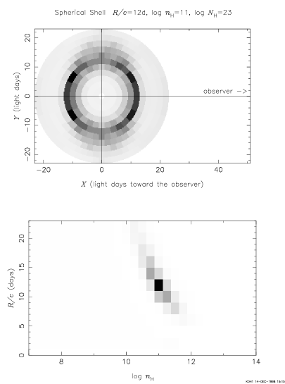
Figure 6: Reconstructed map $\Psi(R,\theta,n)$ of a thin spherical shell (right) from a maximum entropy fit to 7 ultraviolet emission-line lightcurves (left). The light curve fits achieve $\chi^{2}/N=1$. The shell radius $R/c=12$d and density $\log{n}=11$ are correctly recovered. For further details, see text.

In Fig. 6 we present results of a simulation test designed to investigate how well the geometry and physical conditions may be recoverable from reverberations in ultraviolet emission-lines. In this simulation, we assume that clouds with density $n=10^{11}$cm^-3 and column $N=10^{23}$cm^-2 are uniformly distributed over a thin spherical shell of radius $R/c=12$d. An erratically varying source at the centre of the hollow shell drives reverberations in 7 ultraviolet emission lines. We compute the emission-line lightcurves, allowing for light travel time delays and using CLOUDY to account for each line’s anisotropic and non-linear reprocessing efficiency. We sample the synthetic lightcurves at 121 epochs spaced by 2 days, and add noise to simulate observational errors. Finally, we reconstruct a 3-dimensional cloud map $\Psi(R,\theta,n)$ by fitting to the 7 synthetic lightcurves.

It is important to realise that this MEMBLR fit does not assume a spherical shell geometry, but rather it considers every possible cloud map, $\Psi(R,\theta,n)$, and tries to find the “simplest” map that fits the emission-line lightcurves. The fit adjusts 4147 pixels in the cloud map $\Psi(R,\theta,n)$, 143 points in the continuum light curve, $f_{c}(t)$, 7 emission-line background fluxes, $f_{\ell}^{B}(\lambda)$, and 1 continuum flux, $f_{c}^{B}$. This fit assumes the correct column density, $N$, and distance, $D$. The fit to $N=968$ data points achieves $\chi^{2}/N=1$. Entropy maximization “steers” each pixel in the map toward its nearest neighbors, thus giving preference to “smooth” maps, and toward the pixel with the opposite sign of $\cos{\theta}$, thus giving preference to maps with front-back symmetry.

On the left-hand side of Fig. 6, we see that the 8 lightcurves, 7 lines and 1 continuum, are well reproduced by the fit. The highs and lows are a bit more extreme in the data – a common characteristic of regularized fits. To the left of each emission-line light curve, three delay maps are shown corresponding to the maximum brightness (solid curve), minimum brightness (dashed), and the difference (dotted). All the lines exhibit an inward anisotropy except C iii ] . All the lines have positive linear responses except Mg ii , which has a positive response on the near side of the shell and a negative response on the far side.

On the right-hand side of Fig. 6, we see that the fit to the 8 lightcurves recovers a hollow shell geometry with the correct radius. The density-radius projection of the map has a peak at the correct radius and density. The shell spreads in radius by a few light days, with lower densities at larger radii, maintaining a constant ionization parameter.

This simulation test suggests that reverberation effects in the 7 ultraviolet emission-line lightcurves contain enough information to construct useful maps of the geometry and density structure of a photoionised emission-line zone. The 3-dimensional cloud map $\Psi(R,\theta,n)$ clearly recovers the correct hollow shell geometry, the correct radius, and the correct density. The prospects are therefore good for detailed mapping of the geometry and physical conditions in the BLRs of real AGNs. While the current simulation fits only 7 emission-line lightcurves, and demonstrates only 3-dimensional mapping, it is straightforward, though more compute intensive, to add $N$  and $v$ dimensions to the cloud map, synthesize full spectra rather than just line fluxes, and increase the number of lines to several hundred. These extensions should increase the quality of the maps.

4 Summary and Conclusion

Echo tomography is being used to resolve AGN emission-line regions on micro-arcsec scales. In the first decade of echo mapping experiments, datasets have been acquired with great effort through international campaigns focusing on one object per year. The main results are direct measurements of the sizes of broad emission-line regions, several critical tests of photoionisation models (radial ionization structure, luminosity-radius correlation), and rough virial masses for dozens of supermassive black holes.

Our simulation tests illustrate some of the potential future capabilities of echo mapping technology. Future progress depends on facilities like RoboNet and Kronos that are designed for and dedicated to spectrophotometric monitoring of AGNs (and other objects). Delivery of continuous or at least daily records of the evolving spectra over a few hundred days will enable detailed and reliable mapping of broad line regions in up to 5 dimensions, including the geometry ($R,\theta$), kinematics ($v$), and physical conditions ($n_{H}$, $N_{H}$).

Our simulations assume that the physical assumptions and atomic data incorporated into the photoionisation models are correct, and no doubt our knowledge of photoionisation physics, embodied in codes like ION and CLOUDY, will continue to improve through increasingly detailed confrontation with observations. AGNs offer the opportunity to observe and test predictions for the dynamic responses of photoionised gas.

Wavelength-dependent time delays in the AGN continuum should also permit mapping the radial temperature profile $T(R)$ in the continuum production region, which is widely held to be the surface of an accretion disk around the black hole. This method could critically test the accretion disk hypothesis, and may also provide a means of measuring AGN distances to realize their potential as cosmological probes.

- [1] R. D. Blandford and C. F. McKee, “Reverberation mapping of the emission line regions of seyfert galaxies and quasars,” ApJ 255, p. 419, 1982.
- [2] R. Vio, K. Horne, and W. Wamsteker, “Echo mapping of active galactic nuclei broad-line regions: Fundamental algorithms,” PASP 106, pp. 1091–1103, 1994.
- [3] J. H. Krolik and C. Done, “Reverberation mapping by regularized linear inversion,” ApJ 440, pp. 166–180, 1995.
- [4] F. P. Pijpers and I. Wanders, “Reverberation mapping of active galactic nuclei: the sola method for time-series inversion.,” MNRAS 271, pp. 183–196, 1994.
- [5] K. Horne, W. F. Welsh, and B. M. Peterson, “Echo mapping of broad h emission in ngc 5548,” ApJL 367, pp. L5–L8, 1991.
- [6] K. Horne, “Echo mapping problems – maximum entropy solutions,” in Reverberation Mapping of the Broad-Line Region in Active Galactic Nuclei, P. M. Gondhalekar, K. Horne, and B. M. Peterson, eds., ASP Conf. Proc. 69, p. 23, 1994.
- [7] J. Skilling and R. K. Bryan, “Maximum entropy image reconstruction - general algorithm,” MNRAS 211, pp. 111–124, 1984.
- [8] J. H. Krolik, K. Horne, T. R. Kallman, M. A. Malkan, R. A. Edelson, and G. A. Kriss, “Ultraviolet variability of ngc 5548 - dynamics of the continuum production region and geometry of the broad-line region,” ApJ 371, pp. 541–562, 1991.
- [9] A. Wandel, B. M. Peterson, and M. A. Malkan, “Central masses and broad-line region sizes of active galactic nuclei. i. comparing the photoionization and reverberation techniques,” ApJ 526, pp. 579–591, 1999.
- [10] M. H. Ulrich and K. Horne, “A month in the life of ngc 4151: velocity-delay maps of the broad-line region,” MNRAS 283, pp. 748–758, 1996.
- [11] B. M. Peterson and A. Wandel, “Keplerian motion of broad-line region gas as evidence for supermassive black holes in active galactic nuclei,” ApJL 521, pp. L95–L98, 1999.
- [12] B. M. Peterson and A. Wandel, “Evidence for supermassive black holes in active galactic nuclei from emission-line reverberation,” ApJL 540, pp. L13–16, 2000.
- [13] J. H. Krolik, “Systematic errors in the estimation of black hole masses by reverberation mapping,” ApJ 551, pp. 72–79, 2001.
- [14] S. Kaspi, P. S. Smith, H. Netzer, D. Maoz, B. T. Jannuzi, and U. Giveon, “Reverberation measurements for 17 quasars and the size-mass-luminosity relations in active galactic nuclei,” ApJ 533, pp. 631–649, 2000.
- [15] S. J. Collier, K. Horne, I. Wanders, and B. M. Peterson, “A new direct method for measuring the hubble constant from reverberating accretion discs in active galaxies,” MNRAS 302, pp. L24–L28, 1999.
- [16] J. Clavel and et al., “Steps toward determination of the size and structure of the broad-line region in active galactic nuclei. i. an 8 month campaign of monitoring ngc 5548 with iue,” ApJ 366, pp. 64–81, 1991.
- [17] S. Kaspi and H. Netzer, “Modeling variable emission lines in active galactic nuclei: Method and application to ngc 5548,” ApJ 524, pp. 71–81, 1999.