Detailed atmosphere modelling for the neutron star 1E1207.4-5209: Evidence of Oxygen/Neon atmosphere

Abstract

We present a comprehensive investigation of the two broad absorption features observed in the X-ray spectrum of the neutron star 1E1207.4-5209 based on a recent analysis of the 260 ksec XMM-Newton data by Mori et al. 2005. Expanding on our earlier work (Hailey & Mori 2002) we have examined all previously proposed atmospheric models for 1E1207.4-5209. Using our atomic code, which rapidly solves Schrödinger’s equation for arbitrary ion in strong magnetic field (Mori & Hailey 2002), we have systematically constructed atmospheric models by calculating polarization-dependent LTE opacities and addressed all the physics relevant to strongly-magnetized plasmas. We have been able to rule out virtually all atmospheric models because they either do not sustain an ionization balance consistent with the claimed atmosphere composition or because they predict line strengths and line widths which are inconsistent with the data. Only Oxygen or Neon atmospheres at $B\sim 10^{12}$ G provide self-consistent atmospheric solutions of appropriate ionization balance and with line widths, strengths and energies consistent with the observations. The observed features are likely composed of several bound-bound transition lines from highly-ionized oxygen/neon and they are broadened primarily by motional Stark effects and magnetic field variation over the line-emitting region. Further considerations of plausible mechanisms for the formation of a mid-Z atmosphere likely rule out Neon atmospheres, and have important implications for the fallback mechanism in supernova ejecta. Future high resolution spectroscopy missions such as Constellation-X will be able to resolve predicted substructure in the absorption features and will measure magnetic field strength and gravitational redshift independently to better than 10% accuracy.

1 Introduction

Little is known about the surface composition of isolated neutron stars (INS). Strong gravity squeezes NS atmospheres to a thin layer likely composed of a single element (Romani, 1987). Gravitational stratification forces the lightest element to the top of the atmosphere on a time scale of 1–100 sec (Alcock & Illarionov, 1980). It is then likely that the surface is covered by hydrogen. However, various mechanisms can alter the composition from hydrogen. During the supernova explosion, the NS mass cut occurs in the Iron layer (Arnett, 1996). The surface will be covered by iron if there has been no fallback nor accretion. Fallback of supernova ejecta or accretion can put lighter elements on the surface (Woosley & Weaver, 1995). The surface composition can evolve with time via diffuse nuclear burning or excavation by pulsar winds (Chang & Bildsten, 2004). It is impossible to theoretically predict the surface composition of INS as only a tiny amount of material ($\sim 10^{-19}M_{\odot}$) is required to constitute the photosphere.

X-ray spectroscopy is the only tool to probe the surface composition as the surface temperature of observable INS is in the range of $\sim 0.1$–$1$ keV. In particular, detection and identification of spectral features will uniquely determine the surface composition. Nevertheless, previous observations of INS by Chandra and XMM-Newton have somewhat puzzlingly shown no spectral feature (Pavlov et al., 2002; Becker & Aschenbach, 2002). Only recently, a single absorption feature has been detected from several nearby radio-quiet NS (Haberl et al., 2003; van Kerkwijk et al., 2004; Haberl et al., 2004). Although interpretation of these single features is still in debate, they probably indicate presence of light element atmospheres likely composed of hydrogen (van Kerkwijk et al., 2004).

A point source, 1E1207.4-5209, was discovered near the center of the supernova remnant PKS 1209-51 by the Einstein observatory (Helfand & Becker, 1984). The X-ray spectrum is thermal with a temperature $\sim 10^{6}$ K (Vasisht et al., 1997; Zavlin et al., 1998) but no counterpart has been found at other wavelengths yet (Mereghetti et al., 1996). Recent detection of a pulsation period ($P=0.424$ s) provides compelling evidence that 1E1207 is a NS (Zavlin et al., 2000).

1E1207 is unique among thermally-emitting INS because it unambiguously shows two absorption features (Sanwal et al., 2002). It is the first evidence of a non-hydrogenic NS atmosphere (Sanwal et al., 2002) and provides a unique opportunity to use spectroscopy to constrain NS parameters such as magnetic field strength and gravitational redshift. Mereghetti et al. (2002) confirmed the two features in the XMM-Newton/EPIC spectrum. Most recently, Bignami et al. (2003) and De Luca et al. (2004) reported two additional absorption features at 2.1 and 2.8 keV based on the 260 ksec XMM-Newton data. They interpreted the four absorption features as harmonics of electron cyclotron line at $B\sim 8\times 10^{10}$ G. However, Mori et al. (2005) performed a detailed analysis on the 2.1 and 2.8 keV feature and found that they are statistically insignificant and could be related to the instrumental residuals due to Au M-edges.

Since the discovery, various models have been proposed for the 1E1207 absorption features spanning over a wide range of magnetic field strengths and surface compositions. They are Helium atmosphere at $2\times 10^{14}$ G (Sanwal et al., 2002; Pavlov & Bezchastnov, 2005), Iron atmosphere at $\sim 10^{12}$ G (Mereghetti et al., 2002), mid-Z element atmosphere at $\sim 10^{11}$–$10^{12}$ G (Hailey & Mori, 2002), electron cyclotron lines at $\sim 8\times 10^{10}$ G (Bignami et al., 2003; De Luca et al., 2004; Xu, 2005) and Hydrogen molecular ions at $(2-6)\times 10^{14}$ G (Turbiner & López Vieyra, 2004a).

In our previous paper (Hailey & Mori, 2002), we constrained NS atmosphere parameter space and found several solutions that are consistent with the Chandra data. All the solutions were attributed to mid-Z elements. In the present paper we perform a more detailed theoretical analysis of NS atmosphere based on our spectral analysis of the 260 ksec XMM-Newton data (Mori et al., 2005). We concluded that the only plausible solution is an Oxygen or Neon atmosphere at $B\sim 10^{12}$ G.

The outline of the paper is as follows. In §2 we briefly review our spectral analysis of the 260 ksec XMM-Newton data and illustrate the key observables for identifying the spectral features. In §3 we show that modelling of the non-hydrogenic atmosphere using our new atomic code for high magnetic field regime is necessary to interpret the spectral features, in contrast to the previous efforts. We also define NS atmospheric parameter space for our analysis and justify the LTE assumption. In §4 we review atomic physics in the strong magnetic field regime, focusing on feasible spectral features in the X-ray band.

Three major steps follow to constrain the NS parameter space defined in §3. Firstly, we apply the atomic physics methodology to find possible solutions that are consistent with the observed feature location (§5). Some of the solutions were presented in our previous paper (Hailey & Mori, 2002). Secondly, among the potential solutions obtained in §5, we construct an Oxygen atmosphere model at $B=10^{12}$ G (§6). As we will show, this is the only solution consistent with the observed line parameters. Following the partially-ionized magnetized Hydrogen atmosphere models (Potekhin & Chabrier, 2003), we calculate LTE opacities by taking into account all the physics required for the NS atmosphere problem; atomic physics in strong B-field, ionization balance, line broadening and polarization vectors. Thirdly, we critically analyze the other proposed models as well as the other possible solutions from §5 (§7). All the models except O/Ne atmosphere at $B\sim 10^{12}$ G are ruled out based on the NS atmosphere physics addressed in §6 or the existing spectral models with full radiative transfer solutions. Finally, we discuss implications of O/Ne atmosphere in §8 and summarize our results in §9.

2 Data analysis of the 260 ksec XMM-Newton observation

In this section, we briefly summarize our results from the analysis of the 260 ksec XMM-Newton/EPIC data. More details can be found in Mori et al. (2005).

In Mori et al. (2005), we found that two continuum components ($C1$ and $C2$) and two absorption lines ($L1$ and $L2$) are required to fit the data. $C1$/$L1$ and $C2$/$L2$ refer to the lower and higher energy spectral component respectively. The three classes of models are considered (with the notation $C*L$ meaning line $L$ resides on continuum component $C$)

Model I: $$C1*L1*L2+C2$$

Model II: $$C1*L1+C2*L2$$

Model III: $$(C1+C2)*L1*L2$$

Model I assumes that $L1$ and $L2$ are from the same region as the emission of $C1$ and Model II assumes that they are from different regions. Model III assumes that $L1$ and $L2$ are from a layer above the two regions emitting continuum photons.

All the two-component thermal models composed of either blackbody and magnetized Hydrogen atmosphere model fit the data well, yielding a chi-squared very close to unity. For the fit parameters, the reader can refer to table 1 and 2 in Mori et al. (2005). Figure 1 shows the PN singles spectrum fitted by model I with two blackbody components and two Gaussian absorption lines at 0.7 and 1.4 keV. The residuals appear more or less the same for the different fit models and all show an interesting substructure around 0.7 keV in both the PN and MOS data (Mori et al., 2005). Continuum models with power-law components are ruled out because they do not adequately fit the data, leaving significant residuals above 2 keV. When we fit photo-absorption edges to the two absorption features at 0.7 and 1.4 keV, the chi-squared was significantly larger. Therefore we rule out models with photo-absorption edges.

Among the three models described above, we adopt model I to investigate the two absorption features. Model I describes a spectrum composed of a thermal component from a large area on the surface with two absorption features and an additional hot thermal component from a smaller area. The fitted temperature is $\sim 150$–200 eV for the cold thermal component (Note that we converted the best-fit temperature to the NS frame by a gravitational redshift factor $(1+z)=1.3$ which corresponds to $M=1.4M_{\odot}$ and $R=10$ km). The errors in the fitted temperature come primarily from different continuum model fits to the data either by blackbody or magnetized Hydrogen atmosphere models. We found model II implausible from our phase-resolved spectroscopy (Mori et al., 2006). Theoretical models for model III can be found elsewhere (Dermer & Sturner, 1991; Wang et al., 1998; Ruderman, 2003) and we will discuss several cases associated with model III later.

Hereafter we list important observables for identifying the absorption features.

• Equivalent widths of the two features are comparable.

• Line energy ratio of the two features is $\sim 1.9$

• Line energies of the two features are $\sim 0.75$ keV and $\sim 1.4$ keV.

• Line widths ($\equiv\Delta E/E$) are $\sim$40% and $\sim$15% for the 0.7 and 1.4 keV feature.

3 Magnetized non-hydrogenic atmosphere modelling

In principle, the thermal spectrum from a NS is never a blackbody. The atmosphere modifies the spectral energy distribution (SED) and results in the formation of features in the photospheric spectrum. In general, NS atmosphere models are constructed in the parameter space of magnetic field strength ($B$), surface element ($Z$), effective temperature ($T_{eff}$) and gravitational acceleration ($g$) (Becker & Pavlov, 2002).

3.1 Previous approaches: inapplicable to 1E1207

In some special cases, self-consistent NS atmosphere models with full radiative transfer solutions have been constructed with sufficient accuracy for fitting the current X-ray spectroscopic data. However, as we will show, these approaches are not applicable to 1E1207 and magnetic non-hydrogenic atmosphere models are required to interpret the observed spectral features.

Non-magnetic atmosphere models assuming $B=0$ are applicable to NS with $B<10^{9}$ G, such as milli-second pulsars (Zavlin et al., 2002) and accreting NS (Rutledge et al., 1999). At $B<10^{9}$ G, atomic data for $B=0$ case are sufficiently accurate since magnetic field effects do not perturb atomic structure significantly (more details in §4). Sophisticated non-magnetic atmosphere models have been constructed for various atmosphere compositions by implementing reliable opacity libraries such as OPAL (Zavlin et al., 1996; Rajagopal & Romani, 1996; Gänsicke et al., 2002). For any surface composition, non-magnetic atmosphere models do not produce spectral features at 0.7 and 1.4 keV and this is spectroscopic evidence that 1E1207 possesses a magnetic field in excess of $10^{9}$ G.

At $B>10^{9}$ G, modeling NS atmospheres is significantly more difficult because of the complicated magnetic effects on atomic structure and radiation (refer to Lai (2001) for review). In the high B-field regime, only Hydrogen atmospheres have been studied in great detail (Pavlov et al., 1995; Potekhin et al., 1999; Potekhin & Chabrier, 2003, 2004). Partially-ionized Hydrogen atmosphere models show spectral features in the soft X-ray band such as proton cyclotron line, photo-ionization edge or atomic transition lines at $B\>\vbox{\hbox{$>$\hskip-7.5pt\lower 4.30554pt\hbox{$\sim$}}}\>10^{13}$ G (Ho et al., 2003; Ho & Lai, 2004). However, 1E1207 shows absorption features that Hydrogen atmosphere models cannot reproduce. More specifically, the 1.4 keV absorption feature cannot be produced by Hydrogen atoms as the binding energy of a Hydrogen atom never exceeds $\sim 1$ keV at any B-field (Sanwal et al., 2002).

Therefore, a non-hydrogenic magnetized atmosphere model is required to fit the spectral features present in 1E1207 (Sanwal et al., 2002) . However, the few existing non-hydrogenic atmosphere models (Miller, 1992; Rajagopal et al., 1997) are far from complete mainly due to a lack of accurate atomic data for multi-electron ions in the high magnetic field regime.

The model of Miller (1992) and Rajagopal et al. (1997) which utilizes a one-dimensional Hartree-Fock method (Neuhauser et al., 1987) (hereafter 1DHF) is rather crude and the energy values and oscillator strengths have as much as 10% and a factor of 2 uncertainties, respectively. The 10% accuracy of the 1DHF code in transition energies can possibly constrain surface element, but determination of $B$ and $z$ will be inaccurate since they are sensitive to errors in the computed and measured transition energies. The accuracy is unacceptable at the magnetic field strengths and mid-Z elements of interest to us since the 1DHF neglects the effects of excited Landau levels.

Similar problems plague other atomic codes developed for the strong magnetic field regime (Jones et al., 1999; Ivanov & Schmelcher, 2000). They are highly accurate, providing binding energies to better than 0.1% , but their computational speeds are extremely slow because they entail solving the 2-dimensional Schrödinger equation (for detailed comparison of these different atomic calculations, refer to §4 in Mori & Hailey (2002)). They calculate ground state energies of low-Z atoms, but do not provide oscillator strengths. However assessing NS atmospheric conditions requires both transition energies and oscillator strengths for various binding states over a large set of NS parameters.

3.2 Our approach: opacity calculation based on accurate atomic data

Here we utilize an approach for identifying the spectral features based on accurate and extensive atomic data composed of transition energies and oscillator strengths. Our atomic code suitable for the high magnetic field regime provides better than 1% accuracy in transition energies (more details can be found in Mori & Hailey (2002) and §4).

In NS atmosphere spectroscopy, identification of spectral features is further complicated by gravitational redshift ($z$) as it lowers line energies in the observer’s frame by a factor of $(1+z)$. Therefore, spectral feature location depends on the four parameters; $B$, $Z$, number of bound electrons ($n_{e}$) and $z$. Spectral features in the X-ray band emerging from strongly-magnetized plasmas are either cyclotron lines, atomic transition lines or photo-absorption edges. In §5 we investigated any possible combination in the $(B,Z,n_{e},z)$ phase space which generates the observed location of the features. As a result, seven solutions in the $(B,Z,n_{e},z)$ phase space were found by the atomic physics methodology. Derivation of more than one solution is not surprising because we attempt to match two feature locations in the 4-dimensional parameter space of $(B,Z,n_{e},z)$.

One can constrain the NS parameter space further in light of self-consistency and physical plausibility of the models. A self-consistent atmosphere model must solve radiative transfer equations with reliable opacity tables and equation of state as was done for magnetic Hydrogen atmosphere models. Line identification based on transition energies and oscillator strengths presented in §5 is inadequate for NS atmosphere spectroscopy. In the present work, we calculate LTE opacities by taking into account ionization balance and dielectric properties in strongly-magnetized dense plasmas. In the case of 1E1207, opacity highly constrains the NS atmosphere parameter space and leads to a single solution that is physically plausible and consistent with the observed line parameters. As a next step, radiative transfer is in progress using the LTE opacities to construct self-consistent spectral models for fitting to the XMM-Newton data (Mori & Ho, 2006). Nevertheless, our conclusion on the surface composition is unchanged regardless of radiative transfer since our solution is consistent with the observed line parameters over a large range of the NS atmosphere parameters.

Hereafter we briefly review each process involved in computing LTE opacities. In a strong magnetic field, radiation becomes highly anisotropic and propagates in two normal polarization modes (Ginzburg, 1970; Meszaros, 1992). Therefore, opacities are dependent on the direction of photon propagation and the polarization mode. Under the LTE assumption, the absorption opacity $\kappa^{j}(E,\theta_{B},\rho,T)$ [cm²/g] for a photon with energy $E$ propagating in a polarization mode ($j=1,2$) and at an angle $\theta_{B}$ relative to magnetic field is written as (Potekhin & Chabrier, 2003),

$$\kappa^{j}(E,\theta_{B},\rho,T)=M^{-1}\sum_{\alpha}\sum_{i}|\vec{e}_{\alpha}^{j}(E,\theta_{B})|^{2}\sigma^{i}_{\alpha}(E)f_{i}(\rho,T).$$ (1)

$M$ is the atomic mass. $\sigma^{i}_{\alpha}(E)$ is the cross section for an ionization state $i$ and a basic polarization mode $\alpha$. The three basic (cyclic) polarizations ($\alpha=0,\pm 1$) are defined with respect to the magnetic field (one linear along B-field and two circular transverse to B-field). $\sigma^{i}_{\alpha}(E)$ is a quantity derived directly from the Schrödinger equation using our atomic code. $f_{i}$ is the fraction of ionization state $i$, which depends only on plasma density ($\rho$) and temperature ($T$) under the LTE assumption. $f_{i}$ is calculated by solving the Saha-Boltzmann equations modified for strong magnetic regime. $|\vec{e}_{\alpha}^{j}|$ is the projection of the basic polarization vectors in the normal modes, reflecting the dielectric properties of plasma in the magnetic field. We calculate the polarization vectors using the Kramers-Kronig relations adopted for partially-ionized Hydrogen atmosphere models (Bulik & Pavlov, 1996; Potekhin et al., 2004). For some cases, information on the line widths helps to check the plausibility of the models. Various line broadening mechanisms are investigated quantitatively. We emphasize that the procedures presented in this paper were justified and used for constructing partially-ionized Hydrogen atmosphere models in strong magnetic field regime (Potekhin & Chabrier, 2003, 2004). All the physics relevant to strongly-magnetized dense plasmas are addressed in our opacity calculations following Potekhin & Chabrier (2003).

3.3 Range of the atmospheric parameters considered in our analysis

We define the range of NS atmospheric parameters considered in our analysis.

3.3.1 Magnetic field strength

We consider a single value of B-field to identify the observed spectral features. This assumption is valid within a thin photosphere on the NS surface. However, magnetic field can vary over the line-emitting area thus producing line broadening. We will discuss line broadening due to non-uniform B-field distribution in §6.3.5. We investigate a range of magnetic field strength from $B=10^{11}$–$10^{15}$ G in the following analysis. This is the range where our atomic code accurately predicts spectral features for elements $Z=1$–$26$ in the X-ray band. There are several cases which require B-field smaller than $10^{11}$ G, but we can rule out these cases from simple atomic physics arguments.

3.3.2 Atmospheric composition

We consider atmospheres composed of both pure elements and mixtures of different elements in the range of $Z=1$–$26$. We exclude rare elements expected in the products of explosive nucleosynthesis in supernova explosions (e.g. for abundant elements in supernova ejecta, refer to Thielemann et al. (1996)).

3.3.3 Gravitational redshift

We set the range of possible gravitational redshift to $z=0$–$0.85$. The upper bound originates in constraints associated with the nuclear EOS including stability ($dP/d\rho>0$) and causality ($dP/d\rho<c^{2}$ where $c$ is the speed of light) conditions inside the star (Lindblom, 1984; Haensel et al., 1999).

3.3.4 Photosphere temperature

Effective temperature measured from overall spectral fitting is sensitive to assumed atmosphere composition. For 1E1207, $kT_{eff}=150$-$200$ eV covers the whole range of effective temperature. The effective temperature merely represents the total thermal flux, but in reality a NS atmosphere has a temperature gradient under hydrostatic equilibrium. Recent atmosphere modelling showed that absorption features are formed at shallow depths in the photosphere ($\sim(10^{-3}-10^{-1})\tau_{T}$ where $\tau_{T}$ is the Thompson depth). Temperatures at the line forming depths are lower than the effective temperature at most by a factor of few (Ho & Lai, 2001; Miller, 1992). Therefore, we consider a temperature range of $\sim 50$–200 eV. Later in our opacity calculations, we adopt $kT=150$ eV because mid-Z atmospheres generally have a temperature gradient close to the grey profile as bound-bound and bound-free opacities are more important than free-free opacities (Miller, 1992; Rajagopal et al., 1997).

3.3.5 Plasma density

NS photosphere density is roughly in the range of $\sim 10^{0}$–$10^{2}$ g/cm³ depending on surface composition, magnetic field and polarization mode (Pavlov et al., 1995; Becker & Pavlov, 2002; Miller, 1992; Rajagopal et al., 1997). Since absorption lines are formed at smaller optical depths in the photosphere, we focus on a much smaller plasma density range. Hereafter, we consider a density range of $\rho\sim 10^{-4}-10^{2}$ g/cm³ based on Ho & Lai (2001), Ho et al. (2003) and Miller (1992).

3.3.6 LTE consideration

Before proceeding to identify the observed features, we investigate the validity of the local thermodynamics equilibrium (LTE) assumption. LTE greatly simplifies calculation of ionization states and level population as they depend only on plasma density and temperature. In a high density plasma where collisional processes are faster than radiative processes, LTE is well established even for the innermost electron. LTE is achieved when there is simultaneously (1) a Maxwellian electron distribution (2) Saha equilibrium (3) Boltzmann equilibrium (Salzmann, 1998). The conditions for a Maxwellian electron distribution are fulfilled at quite low density since the electron self-collision time is very short (Spitzer, 1962). The range of baryon density considered in our analysis well satisfies conditions for the Saha and Boltzmann equilibrium at $kT=50$–200 eV (Griem, 1964; Salzmann, 1998), hence the NS atmosphere is likely in LTE.

4 Preliminaries for NS atmosphere spectroscopy: Atomic physics in the Landau regime

Before we proceed to constrain the NS atmosphere parameters, we review important magnetic field effects directly relevant to location, strength and width of the observed features.

In a strong magnetic field, atomic structure is quite different from the $B=0$ case. A strong magnetic field deforms the atom to a cylindrical shape when magnetic field effects are larger than Coulomb field effects. This regime (often called the Landau regime) is defined as $\beta_{Z}>1$ where $\beta_{Z}=B/4.7\times 10^{9}Z^{2}$. In the Landau regime the binding energy of bound electrons increases significantly. For instance, the ionization threshold of a Hydrogen atom is 160 eV at $B=10^{12}$ G.

A bound electron in the Landau regime is often denoted by two quantum numbers $m$ and $\nu$ (hereafter we use $(m\nu)$ to denote bound states). $m$ is a magnetic quantum number and $\nu$ is a longitudinal quantum number along the field line. There are two additional quantum numbers, Landau number ($n$) and electron spin component along the field ($s$). They are fixed to $n=0$ and $s=-1/2$ in the Landau regime, where electron cyclotron energy far exceeds Coulomb energy and thermal energy. $\nu=0$ states have larger binding energy (tightly-bound states) and $\nu>0$ states have smaller binding energy (loosely-bound states). In most cases, the ground state configuration is composed of bound electrons in tightly-bound states i.e. $(m0)$ states. The innermost electron is in a $(00)$ state and binding energy of tightly-bound states decreases as $m$ increases. Excited states often involve loosely-bound states (i.e. $(m\nu)$ states with $\nu>0$)

The effects of finite nuclear mass are mentioned here since they help determine the location and width of atomic features. In the absence of a magnetic field, the center-of-mass term and the nucleus-electron term in the Hamiltonian are separated by a canonical transformation. When a magnetic field is present, collective motion of an atom and its internal electric structure are coupled (Pavlov & Meszaros, 1993; Potekhin, 1994) and there remain two additional terms in the transformed Hamiltonian, the nuclear cyclotron term and the motional Stark term (which will be discussed in §6.3.3). Essentially both terms lower the binding energy from that computed from the Hamiltonian with infinite nuclear mass. The nuclear cyclotron term ($=m\hbar\omega_{NB}$ where $\omega_{N}=ZeB/m_{N}c$, $m_{N}$ is the nuclear mass and $c$ is the speed of light) can be simply added to solutions for the infinite nuclear mass case since the term commutes with the Hamiltonian. The combination of the two effects auto-ionizes bound electrons at high magnetic fields (Potekhin, 1994; Kopidakis et al., 1996). Hereafter electron binding energies are computed with a correction for the nuclear cyclotron term. Essentially, the correction to energies (hence oscillator strengths) of $\Delta m\neq 0$ transition lines becomes large at $B>10^{14}$ G, while it is negligible at $B\sim 10^{12}$ G.

4.1 Feasible atomic features in the X-ray band

Feasible atomic transitions in the X-ray band are photo-absorption edges from tightly-bound states or photo-absorption lines from tightly-bound states to tightly-bound states (hereafter tight-tight transition) or loosely-bound states (hereafter tight-loose transition). Landau transitions (between different $n$) and spin-flip transitions (between different $s$) do not occur in a strong magnetic field since they require photon energies comparable to the electron cyclotron energy ($=\hbar\omega_{eB}=11.6B_{12}$ keV and $B=10^{12}B_{12}$ G) to excite the ground states. Nevertheless, we will consider $\Delta n\neq 0$ transitions (the so-called cyclotron lines) as well. An electron spin-flip transition with $\Delta s=1$ has essentially the same line energy as a $\Delta n=1$ transition. However, the line strength of spin-flip transition is significantly smaller than a $\Delta n=1$ transition (Melrose & Zhelezniakov, 1981). Therefore we do not consider the spin-flip transition.

For bound-bound transitions, $\Delta m=0$ and $\Delta\nu=odd$ or $\Delta m=\pm 1$ and $\Delta\nu=even$ transitions are allowed by dipole selection rules (i.e. they have large oscillator strengths) The former transitions occur in the longitudinal polarization mode ($\alpha=0$, parallel to B-field), while the latter transitions occur in the circular polarization mode ($\alpha=\pm 1$, transverse to B-field). Figure 2 shows a Grotrian diagram for strong bound-bound transitions in the Landau regime along with line energies of a H-like oxygen ion at $B=10^{12}$ G.

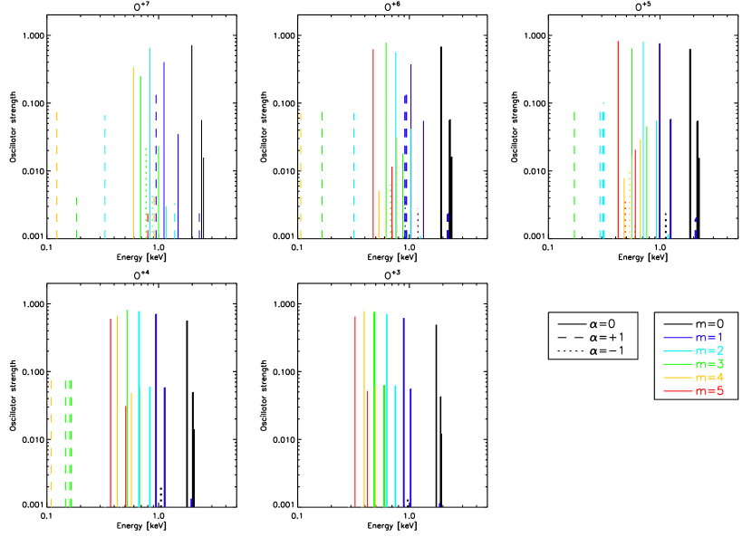
Figure 3: Line spectra of five ionization states of oxygen in the X-ray band at $B=10^{12}$ G. Note that energies are unredshifted. Similar to figure 2, different line types indicate transitions for different cyclic polarization modes. The lines are denoted with different colors according to initial $m$ of a transiting bound electron.

To illustrate transition lines for different polarization modes and initial states, line spectra of five different oxygen ions at $B=10^{12}$ G are shown in figure 3. Strong magnetic field separates different $m$ states and they make groups of transition lines according to different $m$ (denoted by different colors) as seen in figure 3. In this sense, transition lines are evenly distributed in the energy space. This contrasts with the zero magnetic field case in which transitions from the K- and L-shell are largely separated (e.g. 6 keV and 1 keV for K- and L-shell transitions of Iron). In each $m$ group, several tight-loose transitions are feasible but the oscillator strength decreases as $\nu$ becomes larger (Ruder et al., 1994), while in general oscillator strengths for lines depend weakly on $m$ (Miller, 1992; Mori & Hailey, 2002). Separation between the groups of lines becomes smaller as $m$ increases. The line distribution shown in figure 3 is more or less the same for different elements in the Landau regime. We will apply these properties for identifying the observed features from line location and line energy ratio.

4.2 Our atomic code: Multi-configurational, perturbative, hybrid, Hartree, Hartree-Fock method

Identification of atomic features is a time-consuming task requiring a systematic search of the $(B,Z,n_{e},z)$ parameter space. For the purpose of identifying atomic features, we developed a fast and accurate atomic code based with an approach we call multi-configurational, perturbative, hybrid, Hartree, Hartree-Fock theory (hereafter MCPH³) (Mori & Hailey, 2002). For most electron configurations and magnetic field strengths relevant to 1E1207, the MCPH³ code calculates transition energies and oscillator strengths for any given electron configuration of an arbitrary ion in the Landau regime. The MCPH³ code provides atomic data to better than 1% and 10% accuracy for energies and oscillator strengths respectively. The MCPH³ code achieves significantly faster computation time compared to other atomic codes, such as multi-configurational Hartree-Fock codes (Ruder et al., 1994) and two-dimensional Hartree-Fock codes (Ivanov & Schmelcher, 2000), by use of its perturbation method. The resultant fast algorithm of the MCPH³ code enables us to compute atomic data over a large set of $B,Z$ and $n_{e}$ with reasonable CPU time. For instance, computation of a ground state configuration of Oxygen atom (8 bound electrons) was achieved within 5 min on Celeron with 2.4 GHz CPU and 512MB memory. The computation time is roughly proportional to $n_{e}^{2}$ where $n_{e}$ is the number of bound electrons (Mori & Hailey, 2002). We checked that convergence of our atomic calculation was achieved to better than 0.1% by monitoring Hartree energy of each electron orbital. We also extended our atomic code to calculate photo-absorption cross sections and perform molecular structure calculation in the Born-Oppenheimer approximation. Some of the new results are used to constrain the atmosphere models for 1E1207.

4.2.1 Validity range of our atomic code

By applying perturbation methods to higher Landau levels the MCPH³ code has an extended range of applicable magnetic field. The MCPH³ code provides useful results for our analysis (i.e. accuracy in energy of a few%) for $\beta_{Z}\geq 0.3$. This was determined by comparing it with atomic data generated by other approaches (e.g. multi-configurational Hartree-Fork code by Ruder et al. (1994)) known to be highly accurate in the intermediate magnetic field regime ($\beta_{Z}\sim 0.1$–$1$).

On the other hand, relativistic effects become significant at high magnetic field and may affect results from the MCPH³ code, which solves the non-relativistic Schrödinger equation. Transverse motion of electrons around the magnetic field becomes relativistic at $B>4.4\times 10^{13}$ G where the electron cyclotron energy is equal to the electron rest mass energy. The wavefunction of electrons in their transverse direction (the Landau function) has the same form as in the non-relativistic case, as long as electrons are in the ground state of the Landau levels. This is true for the high magnetic fields where the transverse electron motion is relativistic (Lai, 2001). Therefore, relativistic corrections to the transverse motion are irrelevant. On the other hand, bound electrons are subject to a larger nuclear Coulomb field since they are closer to the nucleus at higher magnetic field. Accordingly, relativistic effects significantly affect the longitudinal motion of bound electrons. However, relativistic effects due to the nuclear Coulomb field are negligible as long as the energy range of interest (in our case $\sim 1$ keV) is much smaller than the electron rest energy (Angelie & Deutch, 1978).

As we do not include higher than the 1st order perturbative terms in the electron-electron exchange energy, our atomic calculation becomes less accurate for electron configurations where bound electrons are closer to each other. This is the case for large $m$ states in ground state configurations of ions with many electrons. Accuracy in transition energies and oscillator strengths can drop $\sim$10% and $\sim$50%. However, it does not affect determination of NS atmosphere parameters because the spectral features are due to highly-ionized O/Ne where uncertainty associated with the exchange term is tiny ($<0.1$%).

5 Atomic physics methodology of identifying absorption features

We can constrain the $(B,Z,z,n_{e})$ phase space from the observables presented in §2 and the relevant physical effects discussed in §4. We briefly outline our three-step procedure in connection with the observed properties listed in §2. First, we constrain ionization state ($n_{e}$) from the observation (a), transition energies, oscillator strengths and level population under the LTE assumption. Secondly, we present a scheme to determine magnetic field strength ($B$) from the observation (b). We adopt the line energy ratio as a strong diagnostic parameter to determine $B$ for a given $Z$. $z$ is separately determined from the other parameters since binding energies depend on $B,Z$ and $n_{e}$ in a non-linear fashion, while the gravitational redshift lowers the location of the features linearly by a factor of $(1+z)$. This is different from the case of cyclotron lines where $B$ and $(1+z)$ shift spectral features identically. Finally, we determine surface element ($Z$) from the observation (c), requiring a fit to the features in the XMM-Newton data with a reasonable range of $z$.

Following our previous paper (Hailey & Mori, 2002), we consider three cases; pure atomic transitions (Case A), pure cyclotron transitions (Case B) and a combination of atomic transition and cyclotron line (Case C). In this section, our discussion is mostly devoted to case A. For case B and C, we merely present all the possible solutions and defer more detailed investigation on their plausibility to §7.

The parameter space where we search for plausible solutions is vast and 4-dimensional. Several simple and reasonable assumptions help to significantly reduce the amount of work and time required. Later, we relax the assumptions and consider how this changes the results. We assume a single element and a single ionization state as the zero-th order constraints. The former condition is rather realistic as the gravitational sedimentation is fast on the NS surface. Later we will investigate whether admixtures with more than one element are consistent with the data. In the next section, we relax the latter condition by allowing more than one ionization state while ionization balance will be investigated in §6.2.

5.1 Case A: pure atomic transition lines

In this section we focus on bound-bound transitions for the following reasons, although we considered all combinations of spectral features including bound-free transitions. First, models with photo-absorption edges do not fit the XMM-Newton/EPIC data (Mori et al., 2005). Second, bound-free transitions have significantly smaller cross sections (hence opacities) than bound-bound transitions in the most plausible case (i.e. O/Ne atmosphere at $B\sim 10^{12}$ G) (§6.1).

5.1.1 Constraining ionization state from condition (a)

First of all we constrain the ionization state ($n_{e}$) from the observation (a) that the two features have similar strengths. We examine oscillator strengths of atomic transition lines which may appear in the X-ray band as well as level population from the Boltzmann distribution.

H-like ion

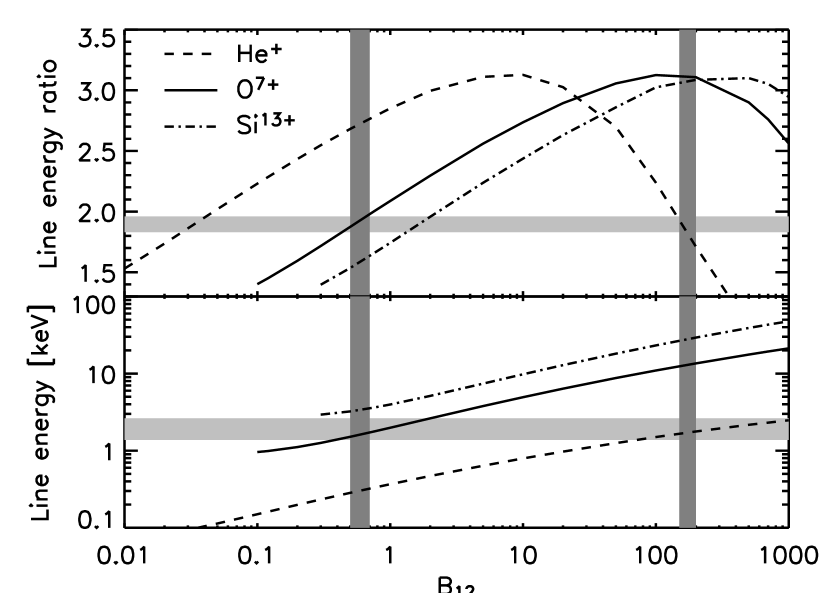
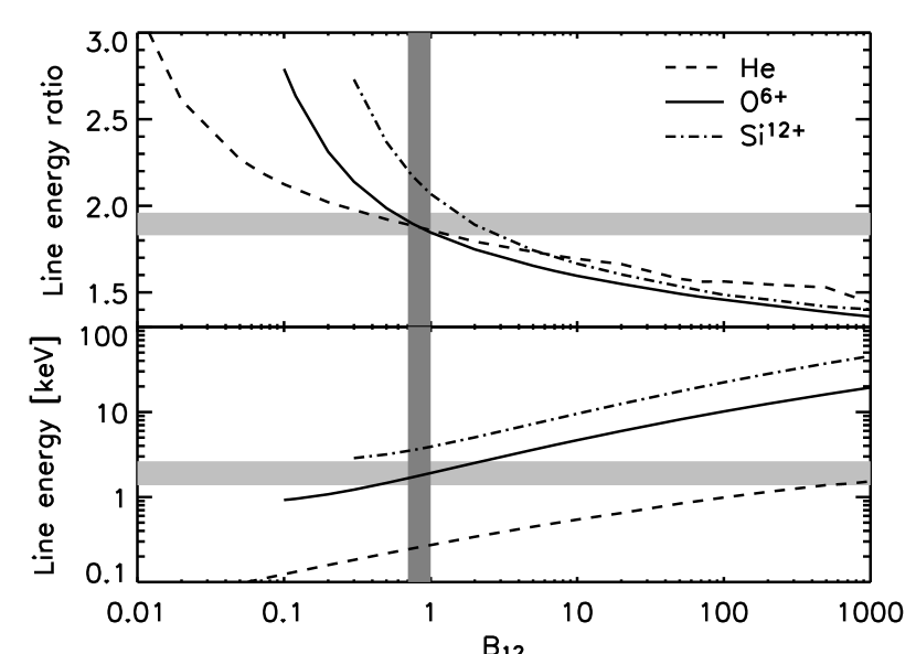
Figure 5: Line energy ratio of H and He-like ions as a function of magnetic field strength. The top figures present the line energy ratios to illustrate condition (b). The bottom figures plot line energies from $(00)\rightarrow(01)$ transition to illustrate condition (c). We considered cases for helium (dashed line), oxygen (solid line) and silicon (dotted-dashed line). For H-like ions, the transition is $(00)\rightarrow(01)$ and $(00)\rightarrow(10)$. For He-like ions, the transition is $(00)(10)\rightarrow(01)(10)$ and $(00)(10)\rightarrow(00)(11)$. The grey areas indicate the measured ratio and energy. Note that line energies are unredshifted and the grey areas are obtained by the measured line energy multiplied by a factor of $(1+z)$ with the range of $z=0$–$0.85$. The black area shows the magnetic field range which satisfies both the line energy ratio (top panel) and transition energy consistent with the XMM-Newton data (bottom panel). Cut-off at lower $B$ indicates that the MCPH³ code provides inaccurate results.

Since the number of observed absorption features is few, we begin with H-like ions. See figure 2 for a Grotrian diagram of H-like oxygen at $B=10^{12}$ G. Ground state configuration of H-like ions consists of $(00)$ state. There are two strong lines from the ground state: $(00)\rightarrow(01)$ and $(00)\rightarrow(10)$ transition. The former is the strongest among tight-loose transitions and its oscillator strength is close to unity. The latter is $\Delta m=+1$ tight-tight transition and its oscillator strength decreases with B-field as $B^{-1}$ (Ruder et al., 1994). In the Landau regime, a line energy ratio of these two transitions is in the range of $\sim 1.5$–3.0 (see §5.1.2 and figure 5), which covers the observed line energy ratio $\sim 1.9$.

Other tight-loose transitions such as $(00)\rightarrow(0\nu)$ with $\nu=3,5...$ or $(00)\rightarrow(1\nu)$ with $\nu=2,4...$ have line energy overlapping with the 0.7 and 1.4 keV feature. However, their oscillator strengths decrease as $(\nu+1)^{-3}$ (Ruder et al., 1994) and high $\nu$ states are possibly destroyed by pressure ionization (§6.2). Therefore tight-loose transitions to higher $\nu$ states are weaker than $\Delta\nu=1$ transitions. This is also true for other ionization states.

The 1st excited state of a H-like ion is $(10)$. Similarly, strong transitions are $(10)\rightarrow(11)$ or $(10)\rightarrow(20)$. $(10)\rightarrow(11)$ transition overlaps with the 0.7 keV feature. $(10)\rightarrow(20)$ transition is irrelevant to the 1E1207 spectrum because it appears below the EPIC band ($E\>\vbox{\hbox{$<$\hskip-7.5pt\lower 4.30554pt\hbox{$\sim$}}}\>0.3$ keV). However, the relative population of the $(10)$ state (1st excited state) to $(00)$ state (ground state) is $\sim\exp{(-\epsilon/kT)}\>\vbox{\hbox{$<$\hskip-7.5pt\lower 4.30554pt\hbox{$\sim$}}}\>10^{-2}$ where $\epsilon\sim 1$ keV is the excitation energy and $kT\>\vbox{\hbox{$<$\hskip-7.5pt\lower 4.30554pt\hbox{$\sim$}}}\>200$ eV. We note that occupation probability of the excited states will be further reduced by pressure ionization (§6.3.2). Therefore, $(10)\rightarrow(11)$ transition will be much weaker than the transitions from $(00)$ state in the 0.7 keV feature. $(10)\rightarrow(02)$ transition is allowed in the $\alpha=-1$ mode. However, transitions in the $\alpha=-1$ mode are in general very weak hence we do not consider them further in this section. We will present cross sections in the $\alpha=-1$ mode in §6.1 and they are included in our opacity calculations.

He-like ion

The ground state configuration of He-like ions is $(00)(10)$. See figure 4 for a Grotrian diagram of He-like oxygen at $B=10^{12}$ G. Tight-loose transitions from the ground state such that $(00)(10)\rightarrow(01)(10)$ and $(00)(10)\rightarrow(00)(11)$ overlap with the 1.4 and 0.7 keV feature respectively. $(00)(10)\rightarrow(00)(20)$ transition appears below the EPIC band.

The 1st excited state of He-like ions is $(00)(20)$ state. Level population relative to the ground state is $\>\vbox{\hbox{$<$\hskip-7.5pt\lower 4.30554pt\hbox{$\sim$}}}\>0.2$ at $kT\>\vbox{\hbox{$<$\hskip-7.5pt\lower 4.30554pt\hbox{$\sim$}}}\>200$ eV. $(00)(20)\rightarrow(01)(20)$ transition overlaps with the 1.4 keV feature. $(00)(20)\rightarrow(00)(21)$ transition appears around 0.5 keV which may partially constitute the 0.7 keV feature. $(00)(20)\rightarrow(10)(20)$ tight-tight transition overlaps with the 0.7 keV feature. The other transitions from the 1st excited state are either very weak or outside the EPIC band.

The 2nd excited state is $(00)(30)$ state with level population $\>\vbox{\hbox{$<$\hskip-7.5pt\lower 4.30554pt\hbox{$\sim$}}}\>0.1$ at $kT\>\vbox{\hbox{$<$\hskip-7.5pt\lower 4.30554pt\hbox{$\sim$}}}\>200$ eV. Similarly, $(00)(30)\rightarrow(01)(30)$ transition overlaps with the 1.4 keV feature, while $(00)(30)\rightarrow(10)(30)$ transition overlaps with the 0.7 keV feature. Transitions from other excited states are unimportant in the X-ray band.

Li-like ion

The ground state configuration of Li-like ions is $(00)(10)(20)$. See figure 4 for a Grotrian diagram of Li-like oxygen at $B=10^{12}$ G. $\Delta\nu=1$ transitions from $(00)$ and $(10)$ overlap with the 1.4 and 0.7 keV feature respectively. Li-like ions have an additional line due to $(20)\rightarrow(21)$ whose transition energy is $\sim$0.5 keV which may merge with the 0.7 keV feature, therefore it is consistent with the data. $(00)(10)(20)\rightarrow(00)(10)(30)$ transition has too low line energy to be observed in the X-ray band. The 1st excited state is $(00)(10)(30)$ with level population $\sim 0.2$ relative to the ground state. Similarly, tight-tight transitions to $(01)(10)(30)$ and $(00)(11)(30)$ will appear in the 1.4 and 0.7 keV feature respectively. We have included other relevant transition lines in our final results.

Be-like ion and other more neutral ions

Ions with more than three electrons (e.g. Be-like ion) may not be plausible simply because additional unobserved features would appear in the EPIC energy band. For instance, Be-like ions will produce a fourth absorption line at $\sim 0.4$ keV due to the $(30)\rightarrow(31)$ transition. $(30)\rightarrow(40)$ transition is located below the EPIC band. Similarly, more neutral ions have $(00)\rightarrow(01)$ transition overlapping with the 1.4 keV feature, while other photo-absorption lines are located below 0.4 keV.

Relaxation of the single ionization state assumption

It is more plausible to interpret the two features as transitions from ions with a few electrons (either H, He and Li-like ion) for the following reasons. The separation in binding energies for two adjacent states is largest for the $(00)$ and $(10)$ states and two adjacent tightly-bound states at $m\geq 2$ do not have a line energy ratio larger than 2. From the measured line energy ratio $\sim 1.9$, we conclude that these two features are from $(00)$ state for H-like ions, $(00)$ and $(10)$ states for He- and Li-like ions because they are the only combination giving the right ratio. For Li-like ions, the 3rd absorption line due to $(20)\rightarrow(21)$ transition may contribute to the 0.7 keV feature. Be-like ions and more neutral ions will show extra absorption features below 0.5 keV. In the next section, we constrain $B$ and $Z$ based on the assumption that the two absorption features are produced by transition lines from highly-ionized atoms.

5.1.2 Constraining magnetic field strength from condition (b)

We constrain magnetic field strength ($B$) from the observation (b) that the measured line energy ratios are $\sim 1.9$. As we discussed in the previous section, the strong absorption lines relevant to the two features are $(00)\rightarrow(01)$ and $(00)\rightarrow(10)$ transition for H-like ions and $(00)(10)\rightarrow(01)(10)$ and $(00)(10)\rightarrow(00)(11)$ transition for He-like ions. Figure 5 shows line energy ratios for H-like and He-like ions of helium, oxygen and silicon as illustrative examples. For H-like ions, there are two solutions: oxygen at $\sim 10^{12}$ G or helium at $\sim 10^{14}$ G. The latter corresponds to the model by Sanwal et al. (2002) and Pavlov & Bezchastnov (2005) . On the other hand, there is only one magnetic field value for a given line energy ratio for He-like ions. For Li-like ions, the 3rd absorption line due to $(20)\rightarrow(21)$ transition contributes to the lower energy line therefore B-field determination will be more complicated.

5.1.3 Constraining atmospheric composition from condition (c)

We constrain atmospheric composition ($Z$) from the observation (c) that the absorption features appear at 0.7 and 1.4 keV. The lower panel in figure 5 shows unredshifted transition energies from the $(00)$ state for H-like ions and the $(00)(10)$ state of He-like ions of helium, oxygen and silicon. Elements above $Z=10$ (e.g. silicon) are excluded because transition energies are too high, which requires unreasonably large gravitational redshift to place lines in the EPIC band.

Searching over $(B,Z)$ phase space in the range of $B=10^{11}$–$10^{14}$ G and $Z=1$–$26$ in the manner described above, the only candidates are oxygen and neon at $B\sim 10^{12}$ G or helium at $B\sim 10^{14}$ G. Note that the Helium solution requires that H-like helium be predominantly populated in the photosphere, while the O/Ne solution allows a range of ionization states. Later, we find the Helium solution implausible on the basis of ionization balance and line strength (§7.1.2). Table 1 shows (unredshifted) line energies for H-, He- and Li-like oxygen. In the Neon case, both magnetic field strength and gravitational redshift are slightly higher than the Oxygen case. For a given element and ionization state, gravitational redshift is simultaneously determined. With the CCD energy resolution, we cannot measure gravitational redshift with high accuracy nor distinguish between Oxygen and Neon models. Here we give the range of the gravitational redshift for each case; $B_{12}\simeq 0.5-1,z\simeq 0-0.4$ for oxygen and $B_{12}\simeq 1-2,z\simeq 0.4-0.8$ for neon.

5.2 Case B: Pure cyclotron lines

We consider the cases involving only cyclotron lines. Unlike case A, here we simply present several possible solutions (see also table 2) and defer discussion on their plausibility to §7.

5.2.1 Electron cyclotron line

The fundamental and 2nd harmonic of electron cyclotron lines have a line energy ratio of two (Xu et al., 2003; Bignami et al., 2003; De Luca et al., 2004). Magnetic field strength is $\sim 8\times 10^{10}$ G to match the observed line energies in 1E1207.

5.2.2 Ion cyclotron line

When $B\>\vbox{\hbox{$>$\hskip-7.5pt\lower 4.30554pt\hbox{$\sim$}}}\>10^{14}$ G, ion cyclotron line energy is in the X-ray band. Unlike electron cyclotron lines, ion cyclotron line energy depends on ionization state and atomic mass ($\hbar\omega_{i}=6.30(Z_{i}/A)B_{12}$ [eV] where $Z_{i}=Z-n_{e}$ and $A$ is atomic number). There are three possible solutions associated with ion cyclotron lines; (1) the fundamental and 2nd harmonics, (2) the fundamental lines from two different elements with atomic mass differ by 2 (e.g. H and He), (3) the fundamental lines from two different charge states (e.g. bare and H-like Helium ion).

5.3 Case C: mixture of atomic transition and cyclotron line

We consider cases in which one of the features is a cyclotron line and the other is an atomic transition line. The ionization state must be hydrogenic since otherwise unobserved features from less ionized states will deviate from the XMM-Newton spectra. As discussed in case A, the feasible atomic transition is either $(00)\rightarrow(10)$ or $(00)\rightarrow(01)$ transition line of H-like ions.

5.3.1 Electron cyclotron line and atomic transition

When the 1.4 keV feature is an electron cyclotron line ($B\sim 2\times 10^{11}$ G), the 0.7 keV feature must be due to either $(00)\rightarrow(01)$ or $(00)\rightarrow(10)$ transition of H-like ion. In either case, the solution requires H-like nitrogen or oxygen.

When the 0.7 keV feature is an electron cyclotron line ($B\sim 8\times 10^{10}$ G), our atomic data is inaccurate for $(00)$ states of mid-Z elements. Hence, we estimated line energies from the atomic data of Ruder et al. (1994) for Hydrogen atom and a well-known scaling law with $Z$ (Ruder et al., 1994). We found that it requires H-like ions of $Z=10$–12.

5.3.2 Ion cyclotron line and atomic transition

In this case, it requires $B>10^{14}$ G to match an ion cyclotron line with one of the two features. The only solution is that the 0.7 keV feature is an ion cyclotron line and the 1.4 keV feature is either $(00)\rightarrow(01)$ transition of H-like helium or $(00)\rightarrow(10)$ transition of H-like lithium at $B\sim 2\times 10^{14}$ G. The former case is nearly identical to the Helium model proposed by Sanwal et al. (2002).

6 Oxygen atmosphere model at B$=10^{12}$ G and $z=0.3$

In this section, we calculate LTE opacities for Oxygen atmosphere at $B=10^{12}$ G and $z=0.3$. $z=0.3$ was chosen so that the calculated line energies roughly match the observed feature energies. We note that all the figures in this section are presented in the observer’s frame after correcting line energies by the redshift factor. We note that the Neon case produces almost identical line energies and opacities with slightly larger $B$ and $z$ values.

6.1 Cross sections

We calculated cross sections for bound-bound transitions and bound-free transitions of all the ionization states of oxygen. Figure 6 shows the cross sections of H-, He-, Li- and Be-like oxygen since we will see later that they are the dominant ionization states in the 1E1207 atmosphere. They are presented for the three cyclic polarization modes ($\alpha=0,\pm 1$) and photon energies are shifted by $(1+z)=1.3$ to roughly match the observed feature energies (indicated by black boxes in the figure). The lines are broad and asymmetric with low energy wings due to motional Stark effects (see §6.3.3). In all the polarization modes, bound-free transitions have much smaller cross sections than bound-bound transitions. The bound-free cross sections are relatively small partially because continuum states are subject to significantly larger motional Stark broadening (Pavlov & Meszaros, 1993). The 1.4 keV feature is mainly composed of $\alpha=0$ transitions along with several weak $\alpha=+1$ transitions. In all the polarization modes, there are a large number of transition lines in 0.5–1.0 keV. Less-ionized oxygen will have more bound-bound transitions below 0.5 keV. We also included the free-free absorption in our model from Potekhin & Chabrier (2003). However, the free-free absorption is unimportant in the X-ray band because the cross sections are significantly smaller than those of bound-bound and bound-free absorption and oxygen is mostly partially-ionized.

6.2 Ionization balance

In this section, we investigate ionization balance of an Oxygen atmosphere at $B=10^{12}$ G. In LTE atmospheres, degree of ionization and level population are determined by the Saha-Boltzmann equilibrium. The generalized Saha equation in the presence of a magnetic field is given by (Khersonskii, 1987; Rajagopal et al., 1997),

$$\frac{n_{i}}{n_{i+1}n_{e}}=\frac{1}{2}\left(\frac{2\pi\hbar^{2}}{m_{e}kT}\right)^{3/2}\frac{\tanh{\eta_{e}}}{\eta_{e}}\frac{\eta_{i}}{\sinh{\eta_{i}}}\frac{\sinh{\eta_{i+1}}}{\eta_{i+1}}e^{\chi_{i}/kT}\frac{Z_{i}}{Z_{i+1}},$$ (2)

where $n_{i}$ is number density of an ionization state $i$, $\eta_{e}=\hbar\omega_{e}/2kT$ and $\eta_{i}=\hbar\omega_{i}/2kT$. $\chi_{i}(>0)$ is the ionization energy. $Z_{i}$ is the internal partition function (IPF) reflecting level population of bound electrons of an ionization state $i$.

In a high density plasma, electron bound states are destroyed (or depopulated) by the electric field from adjacent ions (Pressure ionization). Pressure ionization can be taken into account by assigning occupation probabilities (OP) for bound states

$$Z_{i}=\sum_{\kappa}w_{i,\kappa}g_{i,\kappa}\exp{(-\epsilon_{i,\kappa}/kT)},$$ (3)

where $w_{i,\kappa}$ is the occupation probability and $g_{i,\kappa}$ is the degree of degeneracy of a bound state $\kappa$ of an ionization state $i$. $\epsilon_{i,\kappa}(>0)$ is the excitation energy. Among various approaches for evaluating the OP, we adopted the formalism of Potekhin et al. (2002). We used the fitting formula derived by Potekhin et al. (2002) which reproduce the electric microfield distributions from their Monte-Carlo methods to within a few percent. The microfield distribution of Potekhin et al. (2002) is highly accurate over a large range of the plasma coupling constant ($\Gamma=0$–100). It fully covers the $(\rho,T)$ space discussed in §3.3. We note that the method of Potekhin et al. (2002) also takes into account electron screening of the Coulomb field.

We computed the IPF for each ionization state of oxygen using binding energies calculated by the MCPH³ code. We iteratively solved the coupled Saha equations for different charge states until convergence was achieved. Figure 7 shows the fraction of various ionization states of oxygen for $kT=100$ eV and 200 eV at $B=10^{12}$ G. H, He and Li-like ions for both the Oxygen and Neon case are largely populated at $\rho\sim 10^{-2}$–$10^{0}$ g/cm³ at $kT=100$ eV and $\rho\sim 10^{-2}$–$10^{2}$ g/cm³ at $kT=200$ eV. These temperature and density ranges are typical of the photosphere of 1E1207. To be more realistic, we have calculated ionization fraction for a grey temperature profile at $kT_{eff}=200$ eV. Miller (1992) and Rajagopal et al. (1997) showed that mid-Z element atmospheres have nearly grey temperature profile contrary to Hydrogen or Helium atmospheres because bound-bound and bound-free opacities dominate in mid-Z element atmospheres. Figure 8 shows ionization fraction as a function of optical depth (in units of Thompson depth). Highly-ionized oxygen is largely populated at $\tau=10^{-4}$–$10^{0}$ where the absorption lines are likely formed.

6.3 Line broadening

We investigated various line broadening mechanisms in NS atmospheres. They are compared with the observation (d) that the 0.7 keV feature ($\Delta E/E\sim 40$%) has larger line width than the 1.4 keV feature ($\Delta E/E\sim 15$%). In the opacity calculations, we included all the line broadening effects except magnetic field variation over the line-emission area (hereafter we call it magnetic broadening for convenience) as its distribution is unknown. Nevertheless, we estimated the degree of magnetic broadening in comparison with the XMM-Newton observation. The results are summarized in table 3.

6.3.1 Doppler broadening

For the temperature and spin period of 1E1207, thermal and rotational Doppler broadening are negligible ($\Delta E/E<$ 0.1%).

6.3.2 Pressure broadening

In a dense plasma, electron bound states are perturbed by electric fields from electrons and ions (Salzmann, 1998). The former is caused by the interaction of a radiator with fast free electrons (electron collisional broadening) while the latter is due to the electric field of adjacent ions (quasi-static Stark broadening). Higher excited states are subject to larger broadening. Following Rajagopal et al. (1997), we estimated that pressure broadening produces line broadening of less than 1% for transitions involving $\nu=1,2$ states even at the highest photosphere density ($\rho\sim 10^{2}$ g/cm³). Pressure broadening is not responsible for the broad absorption features.

6.3.3 Motional Stark effects

As ions move randomly in a thermal plasma, coupling of the collective motion and the internal electronic structure induces a motional Stark field ($\vec{E}=\frac{\vec{v}\times\vec{B}}{c}$) in the ion’s comoving frame where $\vec{v}$ is the velocity of ion (i.e. thermal velocity). Since the motional Stark field reduces the binding energy, the line profile has a redward wing (Pavlov & Meszaros, 1993). Line width is estimated as

$$\Delta E_{MS}=kT(1-M_{\perp 1}/M_{\perp 2}),$$ (4)

where $M_{\perp 1}$ and $M_{\perp 2}$ are the so-called anisotropic mass of a ground state and an excited state defined in Pavlov & Meszaros (1993). For each bound state, we evaluated $M_{\perp}$ using the perturbation method adopted by Pavlov & Meszaros (1993). The use of the perturbation method is justified in our case because the atomic mass is much heavier and the binding energies are significantly larger compared to the energy shift caused by the motional Stark field. The estimated line widths are $(10^{-2}-10^{-1})kT$ ($\Delta E/E\>\vbox{\hbox{$<$\hskip-7.5pt\lower 4.30554pt\hbox{$\sim$}}}\>$ few %).

6.3.4 Different ionization states

Lines from different ionization states are likely to contribute to the two broad features because of a temperature gradient in the photosphere. We estimated that line broadening due to different transition lines can be as large as 20% for both features. The 0.7 keV feature will have larger line width than the 1.4 keV feature because $(00)\rightarrow(01)$ transition energies do not vary with ionization states as the transition involves the innermost electron. On the other hand, the 0.7 keV feature consists of many transition lines from different ionization states. This is consistent with the observation (d).

6.3.5 Non-uniform surface magnetic field

The non-uniformity of a surface magnetic field causes line broadening and line energy shift with spin phase since the binding energy is a function of magnetic field. The binding energy of tightly-bound states varies with B-field logarithmically, while the binding energy of loosely-bound states varies even more weakly (Ruder et al., 1994). Therefore, the degree of line broadening is larger for tight-loose transitions. For instance a B-field variation by a factor of 2 (corresponding to the magnetic field difference between the magnetic pole and equator in a dipole configuration) will produce $\sim$ 30% and $\sim 20$% line broadening for tight-loose and tight-tight transitions. However, magnetic broadening alone cannot be responsible for the broad features because the predicted line widths are comparable in both features. Note that phase-resolved spectroscopy can decouple magnetic broadening from other mechanisms since we see different parts of the line-emitting region.

6.4 Polarization vectors

In a strongly-magnetized plasma, radiation propagates in two normal modes: an ordinary mode (O-mode) parallel to the B-field and an extraordinary mode (X-mode) perpendicular to the B-field (Ginzburg, 1970; Meszaros, 1992). The modal description of photon propagation is valid in typical conditions of NS atmosphere except at the resonance energies (e.g. vacuum resonance). Because the X-mode opacities are smaller than the O-mode opacities, X-mode photons decouple from matter at a deeper layer in the atmosphere where the temperature is higher. Therefore, X-ray flux is predominantly carried by the X-mode photons (Shibanov et al., 1992).

We calculated the polarization vectors ($\vec{e}_{\alpha}^{j}$ in equation (1)) following Bulik & Pavlov (1996) and Potekhin et al. (2004). As the Oxygen atmosphere is not fully-ionized, we included effects of the bound species by use of the Kramers-Kronig relation and the absorption coefficients we calculated. Figure 9 shows $|e^{j}_{\alpha}(E)|^{2}$ for X-mode and O-mode at $\theta_{B}=30^{\circ}$, $\rho=0.1$ g/cm³ and $kT=150$ eV. In X-mode, the $\alpha=\pm 1$ vector component is about 1–2 orders of magnitude larger than the $\alpha=0$ vector component over a large range of photon energy and $\theta_{B}$ (photon propagation angle relative to magnetic field). At the resonance energies, spikes are seen due to the large absorption coefficients. We note that even near the resonance energies the modal description is still valid since the polarization vector amplitudes of different basic polarization modes do not cross each other.

6.4.1 Vacuum resonance effects

We briefly describe the effects of vacuum polarization on spectral features as it is important for several proposed models and the few models involving ion cyclotron lines discussed in §5 since they require $B>10^{14}$ G. When $B\>\vbox{\hbox{$>$\hskip-7.5pt\lower 4.30554pt\hbox{$\sim$}}}\>B_{C}$ where $B_{C}=4.414\times 10^{13}$ G, vacuum polarization due to virtual e⁺e^- pairs becomes important. In the photosphere, the effects of the plasma and vacuum polarization become comparable (vacuum resonance) and the two normal modes can switch with each other. The net result is that the X-mode photosphere (where the X-mode photons decouple from matter) is shifted upward in the atmosphere where temperature is lower. As there is less temperature gradient between the X-mode photosphere and the line-forming depth, spectral features are strongly suppressed. Recent Hydrogen atmosphere models with full radiative transfer solutions showed that both ion cyclotron lines and atomic features become unobservable due to the vacuum resonance effects (Ho et al., 2003). We note that the vacuum polarization is negligible for an Oxygen atmosphere at $B\sim 10^{12}$ G.

6.5 LTE opacities

In this section, we present the LTE opacities including all the NS atmosphere physics addressed so far. We fixed $B=10^{12}$ G and $kT=150$ eV to illustrate the density and angular dependence of the opacities. Hereafter we focus on the X-mode opacities since the X-ray flux is predominantly carried by the X-mode photons at $B\sim 10^{12}$ G.

Figure 10 shows X-mode opacities at $\rho=0.1$ g/cm³ (left) and $\rho=10$ g/cm³ (right) respectively ($\theta_{B}=30^{\circ}$). At $\rho=0.1$ g/cm³, $(00)\rightarrow(10)$ transition of H-like oxygen is most prominent in the 0.7 keV feature while the 1.4 keV feature is composed of $(00)\rightarrow(01)$ transition lines of H-like and He-like oxygen. At $\rho=10$ g/cm³, $(00)\rightarrow(01)$ transitions of He- and Li-like ions are strongest in the 1.4 keV feature. Unlike the $\rho=0.1$ g/cm³ case, the 0.7 keV feature consists of tight-loose transition lines of He- and Li-like ions.

Figure 11 shows the X-mode opacities at four different angles. The other parameters are set to the same values ($\rho=1$ g/cm³, $kT=150$ eV and $B=10^{12}$ G) to illustrate the angular dependence. Note that the 1.4 keV feature varies with $\theta_{B}$ more than the 0.7 keV feature because the 1.4 keV feature consists mainly of tight-loose ($\alpha=0$) transitions and their polarization vectors have strong angular dependence. Nevertheless, over a large range of $\theta_{B}$, three complex structures are seen at $\sim$ 0.2, 0.7 and 1.4 keV. These features are robust as they appear over a large range of $\rho,T$ and $\theta_{B}$. The feature at $\sim 0.2$ keV is unobservable by XMM-Newton because the continuum flux is very low at $E\sim 0.2$ keV due to the high ISM neutral Hydrogen absorption. On the other hand, the other two complex features nicely reproduce the two discrete spectral features at $\sim 0.7$ and $\sim 1.4$ keV. They consist of several narrow features, but they may be blurred by the poor CCD resolution. In figure 12 we show the X-mode opacities convolved with the EPIC-PN energy resolution function ($\Delta E/E\sim 5-10$ % (Ehle, 2005)). The 0.7 keV feature has larger line width than the 1.4 keV feature. This is consistent with the observation (d). Magnetic broadening will further broaden both features by roughly the same degree (§6.3.5). Interestingly, the 0.7 keV feature shows substructure, while the 1.4 keV feature appears as a single broad Gaussian-like line. Our spectral analysis of the 260 ksec XMM-Newton data shows a possible substructure in the residuals around 0.7 keV (figure 1). The substructure may indeed reflect the blended lines in the 0.7 keV feature. Investigation of the substructure is in progress with application of the detailed statistical tests following Mori et al. (2005).

7 Investigation of other proposed models

Various models have been proposed for the observed spectral features. We also found several possible solutions involving with cyclotron lines (case B and C). They span over a large range of magnetic fields ($B$) and atomic number ($Z$). We ruled out some cases because self-consistent model spectra with full radiative transfer solutions exist and they do not reproduce the observed line parameters. For the other models, we found them implausible because they lack self-consistency (e.g. ionization balance). Table 2 summarizes all the models and the reasons for implausibility.

7.1 Case A: Pure atomic transition lines

7.1.1 Hydrogen molecular ion model

At a very high B-field, exotic Hydrogen molecules such as H${}_{2}^{+}$, H${}_{3}^{2+}$ and H${}_{4}^{3+}$ become more bound than Hydrogen atoms (Turbiner & López Vieyra, 2004a). Turbiner & López Vieyra (2004a) attributed the observed features to photo-ionization and photo-dissociation of Hydrogen molecular ions at $B=(2-6)\times 10^{14}$ G. They predicted several other spectral features possibly blended in the two broad features.

However, Potekhin & Chabrier (2004) studied ionization balance of a Hydrogen atmosphere at $B\>\vbox{\hbox{$>$\hskip-7.5pt\lower 4.30554pt\hbox{$\sim$}}}\>10^{14}$ G including both atomic and molecular states. They found that the fraction of Hydrogen molecules is negligible and atomic hydrogen is predominantly populated at $T\sim 10^{6}$ K and $B=10^{14}$–$10^{15}$ G. Hydrogen molecules are not abundant enough to produce observable absorption features in the spectra. Atomic hydrogen alone cannot produce spectral features at the observed energies. At $B\>\vbox{\hbox{$>$\hskip-7.5pt\lower 4.30554pt\hbox{$\sim$}}}\>10^{14}$ G, spectral features from atomic hydrogen as well as proton cyclotron lines are significantly suppressed due to vacuum resonance effects (Ho et al., 2003).

7.1.2 Helium atmosphere model

Sanwal et al. (2002) and Pavlov & Bezchastnov (2005) interpret the two features as atomic transition lines from once-ionized Helium ions at $B=2\times 10^{14}$ G. The transitions considered by Pavlov & Bezchastnov (2005) are the $(00)\rightarrow(01)$ and $\Delta m=1$ transition with an increment in another quantum number associated with ionic motion for the 1.4 keV and 0.7 keV feature (Pavlov & Bezchastnov, 2005). They predicted several transition lines possibly blended in the 0.7 keV feature.

At such high B-field, the X-ray continuum flux is carried exclusively by X-mode photons. Adopting the oscillator strengths of the relevant transition lines from Pavlov & Bezchastnov (2005), we calculated X-mode opacities. We found that the $(00)\rightarrow(01)$ transition line is approximately 2 orders of magnitude smaller than the $(00)\rightarrow(10)$ transition line at very small $\theta_{B}$ and $(00)\rightarrow(01)$ transition is completely suppressed at $\theta_{B}\>\vbox{\hbox{$>$\hskip-7.5pt\lower 4.30554pt\hbox{$\sim$}}}\>10^{\circ}$. The suppression of tight-loose transitions is due to the extremely large polarization ellipticity at $B>10^{14}$ G. It is inconsistent with the comparable line strengths of the two features (observation (a)). This conclusion is robust regardless of ionization balance and level population.

The model of Pavlov & Bezchastnov (2005) requires that He⁺ ions largely populate the atmosphere. However that may not be the case as He atoms may be abundant and even He molecules may be formed at $B>10^{14}$ G. Turbiner & López Vieyra (2004b) has shown that He${}_{2}^{3+}$ ion is the most bound system at $B>10^{14}$ G. Using our atomic code modified for molecular structure calculations (Mori & Hailey, 2002), the dissociation energy of Helium molecules is $\sim$2 keV at $B\sim 2\times 10^{14}$ G. This is consistent with the results of Lai (2001). Since the thermal energy in the 1E1207 atmosphere ($kT\>\vbox{\hbox{$<$\hskip-7.5pt\lower 4.30554pt\hbox{$\sim$}}}\>200$ eV) is $\>\vbox{\hbox{$<$\hskip-7.5pt\lower 4.30554pt\hbox{$\sim$}}}\>10$% of the dissociation energy, molecular chains may well be formed (Lai, 2001). Therefore, transition lines from He molecules will produce absorption features at different energies from the observed location.

In addition, vacuum resonance effects may be effective and suppress spectral features as the vacuum polarization becomes important at $B>10^{14}$ G.

7.1.3 Iron atmosphere model

Mereghetti et al. (2002) suggested an Iron atmosphere at $B\sim 10^{12}$ G, although they did not show transition energies corresponding to the observed features. We investigated different ionization states of iron at $B\sim 10^{12}$ G, and the only possible combination of transition lines giving the measured line energy ratio is related to the $(00)$ and $(10)$ states. However, for all the ionization states, the binding energy of these states exceeds 10 keV (e.g. $E>1$ MeV for highly-ionized iron at $B\sim 10^{12}$ G). Therefore it is impossible to match them to the observed features for any reasonable value of gravitational redshift. Iron atmosphere should show far more than the two discrete features in the X-ray band (Rajagopal et al., 1997).

7.2 Case B: Pure cyclotron line case

We find all the pure cyclotron line cases implausible because they are inconsistent with the observed line strengths and widths. Both electron and ion cyclotron lines have been previously studied in great detail and none of the models is consistent with the XMM-Newton data.

7.2.1 Electron cyclotron line

Sanwal et al. (2002) ruled out the electron cyclotron line model because the 2nd harmonic has significantly smaller line strength than the fundamental at $B\sim 8\times 10^{10}$ G. However, Xu (2005) argued that electron cyclotron resonant scattering may modify line strengths resulting in similar strength in the fundamental and the 2nd harmonics.

Radiative transfer models of electron cyclotron lines including the effects of resonant scattering have been extensively studied for various physical conditions ranging from NS binaries to gamma-ray bursts (Alexander & Meszaros, 1989; Wang et al., 1993; Fenimore et al., 1988; Freeman et al., 1999). We extrapolated these models (especially a semi-analytical model by Wang et al. (1993), hereafter W93) to $B\>\vbox{\hbox{$<$\hskip-7.5pt\lower 4.30554pt\hbox{$\sim$}}}\>10^{11}$ G, significantly lower B-fields than the NS binary cases.

We assume a thin isothermal layer composed of fully-ionized plasma with uniform B-field. We assume that the line-forming plasma is cold (i.e. $kT\ll\hbar\omega_{eB}$). This simple picture well represents the proposed electron cyclotron line scenarios either by a layer of e⁺e^- or e-p pairs above the NS surface sustained by radiation pressure (De Luca et al., 2004) or a thin electrosphere on the surface of bare quark stars (Xu, 2005). The corresponding fit model is model III and the fitted optical depth ($\tau$) to the XMM-Newton data is $\sim 0.5$ for the both features (Mori et al., 2005).

Line strength

Electron cyclotron lines ($\Delta n\neq 0$ transitions) are resonant lines because de-excitation of electrons from the higher Landau levels is instantaneous (Harding & Daugherty, 1991). Electrons in $n=1$ states can de-excite only to $n=0$ states, while electrons in $n=2$ states can either de-excite directly to $n=0$ states or deexcite to $n=1$ states then to $n=0$ states (Raman scattering) (W93). The fraction of Raman-scattered photons from the $n=2$ state is given by $1-B/B_{c}$ (Daugherty & Ventura, 1977). At $B\>\vbox{\hbox{$<$\hskip-7.5pt\lower 4.30554pt\hbox{$\sim$}}}\>10^{11}$ G, electrons in $n=2$ states will undergo Raman scattering with probability close to unity. This means that the 2nd harmonic line is absorption-like without suffering from significant resonant scattering. The fitted optical depth of the 1.4 keV feature immediately gives the electron column density of $N_{e}\sim 10^{20}$ cm^-2 (W93).

On the other hand, the fundamental absorption line is subject to two different resonant scattering processes: (1) a photon from $n=1\rightarrow 0$ de-excitation and (2) multiple photons from the Raman scattering from $n>1$ states. The latter process is called “spawning” (W93). At $N_{e}\sim 10^{20}$ cm^-2, we estimated the fraction of spawned photons is only $\sim 10$% (W93). The negligible spawning is due to the fact that the 2nd harmonic line is optically thin. On the other hand, the optical depth of the fundamental line is very large ($\tau\sim 400$) at $N_{e}\sim 10^{20}$ cm^-2 (W93). A similar case with such a large optical depth for the fundamental line is well illustrated in the three right panels in figure 1 of W93. The figure shows the case of $N_{e}=1.2\times 10^{22}$ cm^-2 and $B=1.2\times 10^{12}$ G without spawning (accordingly $\tau\sim 300$ for the fundamental line). We note that the model of W93 takes into account full radiative transfer with resonant scattering. At any viewing angle $\theta_{B}$, the fundamental line appears very deep with the optical depth far exceeding 1. This is inconsistent with the observed optical depth of the 0.7 keV feature ($\tau\sim 0.5$).

Line width

Line widths of the electron cyclotron lines are primarily determined by the B-field variation over the line-forming region, especially when the lines are as broad as the 1E1207 case. As the cyclotron line energy is proportional to $B$, $\Delta E/E$ $(\sim\Delta B/B)$ must be same for the fundamental and 2nd harmonic. This is inconsistent with the observation (d).

7.2.2 Ion cyclotron line

Ion cyclotron lines have been studied in great detail at $B>10^{14}$ G (Zane et al., 2001; Özel, 2001; Ho & Lai, 2003). Ion cyclotron lines at $B>10^{14}$ G are unlikely to be observable since they are significantly weakened by vacuum resonance effects in the photosphere (Ho & Lai, 2003). Similar to the electron cyclotron case, the line width argument makes the ion cyclotron line solutions implausible as well.

7.3 Case C: mixture of atomic transition and cyclotron line

All the case C solutions require a large population of H-like ions in the photosphere because otherwise less ionized states will produce unobserved features in the X-ray band. The solutions with an electron cyclotron line are either nitrogen/oxygen at $B\sim 2\times 10^{11}$ G or $Z=10$–12 element at $B\sim 8\times 10^{10}$ G. However, based on the ionization balance calculation described in §6.2, we found that more neutral ions are predominantly populated in the $(\rho,T)$ range of the 1E1207 photosphere. The solutions with an ion cyclotron line require either a Helium or Lithium atmosphere at $B\sim 2\times 10^{14}$ G. In the former case, He molecular states are predominantly populated (§7.1.2). We ruled out the latter case because H-like Li ions are not abundant at all in the photosphere and also because Lithium abundance is extremely low in the predicted compositions of supernova ejecta (Thielemann et al., 1996).

8 Implications of an Oxygen/Neon atmosphere

The presence of an O/Ne atmosphere makes 1E1207 unique while other INS are likely to have light element atmospheres composed of hydrogen or helium. There are several possible scenarios for the formation of an O/Ne atmosphere. O/Ne may be continuously supplied to the surface by accretion. As accretion flow from the ISM contains different elements (e.g., H, He, CNO), and a mixture of atmospheric elements is expected in the photosphere. In that case, other elements such as carbon and nitrogen and possibly helium will produce unobserved spectral features in the X-ray band. Therefore, we do not consider the accretion scenario plausible. We also note that radiative levitation of O/Ne ions is not effective as the radiative pressure by thermal flux is insufficient. Therefore, it is natural to assume that 1E1207 has a pure O/Ne atmosphere.

An O/Ne atmosphere could be formed by fallback after a supernova explosion (Herant & Woosley, 1994). O/Ne must have survived spallation and soft-landed on the NS surface (Chang & Bildsten, 2004). In the supernova ejecta, oxygen is a dominantly abundant element over a wide range of progenitor mass (Thielemann et al., 1996), so it is feasible that oxygen would appear on the NS surface rather than neon. Optical observations establish the existence of oxygen in the vicinity of 1E1207 (Ruiz, 1983). The high galactic latitude of the supernova remnant PKS 1209-51 indicates an Oxygen-rich environment around the pulsar (Ruiz, 1983). The fallback scenario rules out a Neon atmosphere and favors a pure Oxygen atmosphere.

Post-supernova mixing of the ejecta must occur so that oxygen can diffuse closer to the NS and eventually fall onto the surface. Large-scale mixing is supported both by observations (Spyromilio, 1994; Fassia et al., 1998) and simulations (Hachisu et al., 1992, 1994; Herant & Woosley, 1994). Recent two-dimensional simulations have shown shortly after a supernova explosion oxygen quickly diffuses toward the remnant by Rayleigh-Tailor instabilities (Kifonidis et al., 2000, 2003). In several particular case simulated by Kifonidis et al. (2000) and Kifonidis et al. (2003), oxygen and helium are the most abundant elements in the vicinity of the NS. Note that the degree of mixing will depend on various factors such as progenitor mass, delay time of neutrino-driven explosion and mass-cut location (Kifonidis et al., 2003).

Along with oxygen, other elements such as hydrogen and helium could also fall back onto the surface. Chang & Bildsten (2004) showed a Hydrogen layer could be completely depleted by diffusive nuclear burning within 7 kyrs (i.e. the age of 1E1207 estimated from the surrounding supernova remnant). Their calculation was performed specifically for 1E1207 by using the NS parameters determined by our present analysis. Therefore, fallback of hydrogen is not a problem for 1E1207. On the other hand, the Helium abundance in the photosphere must be negligible ($\ll 10^{-19}M_{\odot}$), otherwise the Helium layer must be depleted by another mechanism (e.g., pulsar wind) over the last 7 kyrs. Chang & Bildsten (2004) estimated that the column density excavated by pulsar winds is comparable with the amount of hydrogen or helium in radio pulsars. However, the excavation occurs only at the polar cap area as ions are ripped off from the surface along open field lines. Since the polar cap size of 1E1207 is small (less than 1km in radius), it is inconsistent with the presence of the absorption features in all spin phases (De Luca et al., 2004) unless special geometry is invoked.

Therefore, it is more natural to assume that a pure Oxygen layer was formed soon after the supernova explosion. Presence of oxygen on the surface of 1E1207 puts stringent conditions on the post-supernova environment and the fallback mechanism. All of the following processes (i.e. formation of NS, mixing of an Oxygen shell toward the NS, negligible Helium contamination and soft-landing of Oxygen nuclei without spallation) must occur after the supernova explosion.

9 Summary

• An O/Ne atmosphere at $B\sim 10^{12}$ G is the only consistent solution with the observed line parameters.

• Other proposed models are ruled out either because they are inconsistent with the observed line parameters or because they lack self-consistency (e.g. ionization balance).

• The magnetic field strength and gravitational redshift are uniquely determined: $B_{12}\simeq 0.5$–$1.0,z\simeq 0$–$0.4$ for oxygen, and $B_{12}\simeq 1.0$–2.0, $z\simeq 0.4$–0.8 for neon.

• The two broad features are due to bound-bound transitions from highly-ionized O/Ne. Bound-free and free-free absorption are not important.

• Highly-ionized (H-, He- and Li-like) O/Ne are largely populated in the photosphere.

• The observed features are broad due to motional Stark effects and magnetic field variation over the surface.

• Several photo-absorption lines from different O/Ne ions are blended in the two features. In our model, the 0.7 keV feature has larger line width than the 1.4 keV feature and may show substructure in the XMM-Newton/EPIC spectra because it contains more blended absorption lines.

• Mixed atmosphere composition is allowed only with hydrogen and only if O/Ne is continuously supplied by accretion. However, the admixture atmosphere case is implausible because accretion flow from the ISM will contain other mid-Z elements (e.g. carbon and nitrogen).

• Fallback of supernova ejecta is the most plausible scenario for the formation of an O/Ne atmosphere. A Neon atmosphere is ruled out because the Neon abundance is much smaller than the Oxygen abundance in the supernova ejecta. Large-scale mixing of supernova ejecta and soft-landing fallback of oxygen with negligible Helium contamination must have occurred after the explosion.

In the present analysis, we have constrained the surface composition of 1E1207 using the CCD spectroscopy aboard XMM-Newton telescope. Resolving blended lines by high resolution grating spectroscopy will lead to highly accurate measurements of magnetic field strength and gravitational redshift to better than 10% accuracy. Phase-resolved spectroscopy will possibly decouple magnetic field effects from gravitational effects because the magnetic field varies with spin phase, while gravitational redshift does not. Radiative transfer using the LTE opacities is in process for calculating self-consistent temperature profiles and emergent spectra (Mori & Ho, 2006). Our spectral models will be fitted to the XMM-Newton data and determine NS parameters.

Figure 1: XMM-Newton/EPIC PN-singles (left) and MOS (right) spectrum and residuals. We fit the spectra with model I with two blackbody components and two Gaussian absorption lines at $\sim 0.7$ and $\sim 1.4$ keV. For the MOS spectrum, we combined MOS1 and MOS2 data to improve photon statistics. An interesting substructure is seen around 0.7 keV in both PN and MOS spectrum.

Figure 2: Grotrian diagram for strong transitions in the Landau regime. The solid, dashed and dotted lines denote transitions for $\alpha=0,+1$ and $-1$ mode respectively. (Unredshifted) transition energies [keV] of H-like oxygen at $B=10^{12}$ G are also shown next to the arrows (large and small font size correspond to transition energies from ground states and excited states respectively). The ground state ($(00)$ state for H-like oxygen) is indicated by a bold horizontal line.

Figure 4: Grotrian diagram for strong transitions of He-like (left) and Li-like (right) oxygen at $B=10^{12}$ G. See the caption of figure 2 for notations.

Figure 6: Bound-bound and bound-free transition cross sections of H-, He-, Li- and Be-like oxygen for $\alpha=0$ (left), $\alpha=+1$ (middle) and $\alpha=-1$ (right) polarization mode at $B=10^{12}$ G. Photon energies are shifted by $(1+z)=1.3$. The observed feature energies are indicated by black boxes. All the ions are assumed to have the same ionization fraction. For transition lines from excited states, we multiplied oscillator strengths by the Boltzmann factors assuming $kT=150$ eV.

Figure 7: Ionization balance of oxygen at $B=10^{12}$ G and $kT=100$ eV (left) and $kT=200$ eV (right). The dotted curve shows the summed ionization fraction from B-like to neutral oxygen.

Figure 8: Ionization fraction of oxygen for the grey temperature profile at $kT_{eff}=200$ eV and $B=10^{12}$ G. The dotted curve shows the summed ionization fraction from B-like to neutral oxygen.

Figure 9: Squared amplitude of the basic polarization vectors for X-mode (left) and O-mode (right) at $\theta_{B}=30^{\circ}$, $\rho=0.1$ g/cm³ and $kT=150$ eV. Solid, dashed and dotted lines indicate longitudinal ($\alpha=0$), right-circular ($\alpha=+1$) and left-circular ($\alpha=-1$) polarization respectively. The spikes are due to the resonant behavior of the dielectric tensors at the transition energies.

Figure 10: X-mode opacities of oxygen at $\rho=0.1$ g/cm³ (left) and $\rho=10$ g/cm³ (right). The other parameters are $B=10^{12}$ G, $kT=150$ eV and $\theta_{B}=30^{\circ}$.

Figure 11: X-mode opacities of oxygen at four different angles ($\theta_{B}=10,30,60$ and 80^∘). The other parameters are $B=10^{12}$ G, $kT=150$ eV and $\rho=1$ g/cm³.

Figure 12: X-mode opacities in figure 10 ($\rho=10$ g/cm³) blurred by XMM-Newton/EPIC energy resolution function.

Table 1: Unredshifted line energies [keV] for H-, He- and Li-like oxygen in the range of $B_{12}=0.5$–1.

Transition	$(00)\rightarrow(01)$	$(00)\rightarrow(10)$	$(10)\rightarrow(11)$	$(10)\rightarrow(02)$	$(20)\rightarrow(21)$	$(20)\rightarrow(12)$
Which feature?	1.4 keV	0.7 keV	0.7 keV	0.7 keV	0.7 keV	0.7 keV
Polarization mode ($\alpha$)	0	+1	0	-1	0	-1
O VIII	1.51–1.98	0.81–0.95	0.79–1.12	0.96–1.32	0.58–0.84	0.74–1.04
O VII	1.46–1.91	0.77–0.91	0.74–1.03	0.87–1.19	0.52–0.76	0.65–0.92
O VI	1.42–1.84	0.76–0.89	0.71–0.99	0.82–1.12	0.49–0.71	0.60–0.83

Table 2: Check list of all the models considered.

Case	Element	Ionization states	B [G]	0.7 keV	1.4 keV	Why implausible?
A	O or Ne	H-, He-, Li-like	$10^{12}$	L	L	OK
A	H	H${}_{3}^{2+}$, H${}_{4}^{3+}$	$4\times 10^{14}$			IB & VR
A	He	H-like	$2\times 10^{14}$	L	L	LS, IB & VR
A	Fe	unknown	$10^{12}$	?	?	Too many features
B	–	Fully-ionized	$8\times 10^{10}$	EC	EC	LS & LW
B	–	Fully-ionized	$6\times 10^{14}$	IC	IC	LS & LW
C	N or O	H-like	$10^{11}$	L	EC	IB
C	Ne, Na or Mg	H-like	$8\times 10^{10}$	EC	L	IB
C	He or Li	H-like	$2\times 10^{14}$	L	IC	IB & VR

Note. — L - photo-absorption line, EC - electron cyclotron line and IC - ion cyclotron line, LS - Line strength, LW - Line width, IB - Ionization balance and VR - Vacuum resonance effect

Table 3: Estimated line widths ($\Delta E/E$ [%]) by various line broadening mechanisms.

Mechanism	0.7 keV	1.4 keV	Relevant parameters
Doppler broadening	$<0.1$	$<0.1$	$T$, spin period
Pressure broadening	$<1$	$<1$	$\rho,T$
Motional Stark broadening	$<$$\sim$  5	$<$$\sim$  1	$B$, $T$
Different ionization states	$\>\vbox{\hbox{$<$\hskip-7.5pt\lower 4.30554pt\hbox{$\sim$}}}\>20$	$\>\vbox{\hbox{$<$\hskip-7.5pt\lower 4.30554pt\hbox{$\sim$}}}\>20$	$B$, $T$
B-field variation	$\sim 7$–14	$\sim 12$	$B$

Note. — The measured line widths are $\sim 40$ % and $\sim 15$ % for the 0.7 and 1.4 keV feature.

References

- Alcock & Illarionov (1980) Alcock, C. & Illarionov, A. 1980, ApJ, 235, 534
- Alexander & Meszaros (1989) Alexander, S. G. & Meszaros, P. 1989, ApJ, 344, L1
- Angelie & Deutch (1978) Angelie, C. & Deutch, C. 1978, Phys. Lett. A, 67, 353
- Arnett (1996) Arnett, D. 1996, Supernovae and nucleosynthesis. an investigation of the history of matter, from the Big Bang to the present (Princeton series in astrophysics, Princeton, NJ: Princeton University Press, —c1996)
- Becker & Aschenbach (2002) Becker, W. & Aschenbach, B. 2002, Proceedings of the 270.WE-Heraeus Seminar on Neutron Stars, Pulsars and Supernova Remnants, Jan21-25, Physikzentrum Bad Honnef, preprint (astro-ph/0208466)
- Becker & Pavlov (2002) Becker, W. & Pavlov, G. G. 2002, The Century of Space Science, eds. J. Bleeker, J. Geiss, M. Huber, Kluwer Academic Publishers, in press (astro-ph/0208356)
- Bignami et al. (2003) Bignami, G. F., Caraveo, P. A., Luca, A. D., & Mereghetti, S. 2003, Nature, 423, 725
- Bulik & Pavlov (1996) Bulik, T. & Pavlov, G. G. 1996, ApJ, 469, 373
- Chang & Bildsten (2004) Chang, P. & Bildsten, L. 2004, ApJ, 605, 830
- Daugherty & Ventura (1977) Daugherty, J. K. & Ventura, J. 1977, A&A, 61, 723
- De Luca et al. (2004) De Luca, A., Mereghetti, S., Caraveo, P. A., Moroni, M., Mignani, R. P., & Bignami, G. F. 2004, A&A, 418, 625
- Dermer & Sturner (1991) Dermer, C. D. & Sturner, S. J. 1991, ApJ, 382, L23
- Ehle (2005) Ehle, M. e. a. 2005, XMM-Newton Users’ Handbook
- Fassia et al. (1998) Fassia, A., Meikle, W. P. S., Geballe, T. R., Walton, N. A., Pollacco, D. L., Rutten, R. G. M., & Tinney, C. 1998, MNRAS, 299, 150
- Fenimore et al. (1988) Fenimore, E. E., Conner, J. P., Epstein, R. I., Klebesadel, R. W., Laros, J. G., Yoshida, A., Fujii, M., Hayashida, K., Itoh, M., Murakami, T., Nishimura, J., Yamagami, Y., Kondo, I., & Kawai, N. 1988, ApJ, 335, L71
- Freeman et al. (1999) Freeman, P. E., Lamb, D. Q., Wang, J. C. L., Wasserman, I., Loredo, T. J., Fenimore, E. E., Murakami, T., & Yoshida, A. 1999, ApJ, 524, 772
- Gänsicke et al. (2002) Gänsicke, B. T., Braje, T. M., & Romani, R. W. 2002, A&A, 386, 1001
- Ginzburg (1970) Ginzburg, V. L. 1970, The propagation of electromagnetic waves in plasmas (International Series of Monographs in Electromagnetic Waves, Oxford: Pergamon, 1970, 2nd rev. and enl. ed.)
- Griem (1964) Griem, H. R. 1964, Plasma spectroscopy (New York: McGraw-Hill, 1964)
- Haberl et al. (2003) Haberl, F., Schwope, A. D., Hambaryan, V., Hasinger, G., & Motch, C. 2003, A&A, 403, L19
- Haberl et al. (2004) Haberl, F., Zavlin, V. E., Trümper, J., & Burwitz, V. 2004, A&A, 419, 1077
- Hachisu et al. (1992) Hachisu, I., Matsuda, T., Nomoto, K., & Shigeyama, T. 1992, ApJ, 390, 230
- Hachisu et al. (1994) —. 1994, A&AS, 104, 341
- Haensel et al. (1999) Haensel, P., Lasota, J. P., & Zdunik, J. L. 1999, A&A, 344, 151
- Hailey & Mori (2002) Hailey, C. J. & Mori, K. 2002, ApJ, 578, L133
- Harding & Daugherty (1991) Harding, A. K. & Daugherty, J. K. 1991, ApJ, 374, 687
- Helfand & Becker (1984) Helfand, D. J. & Becker, R. H. 1984, Nature, 307, 215
- Herant & Woosley (1994) Herant, M. & Woosley, S. E. 1994, ApJ, 425, 814
- Ho & Lai (2001) Ho, W. C. G. & Lai, D. 2001, MNRAS, 327, 1081
- Ho & Lai (2003) —. 2003, MNRAS, 338, 233
- Ho & Lai (2004) —. 2004, ApJ, 607, 420
- Ho et al. (2003) Ho, W. C. G., Lai, D., Potekhin, A. Y., & Chabrier, G. 2003, ApJ, 599, 1293
- Ivanov & Schmelcher (2000) Ivanov, M. V. & Schmelcher, P. 2000, Phys. Rev. A, 61, 022505
- Jones et al. (1999) Jones, M. D., Ortiz, G., & Ceperley, D. M. 1999, Phys. Rev. A, 59, 2875
- Khersonskii (1987) Khersonskii, V. K. 1987, AZh, 64, 433
- Kifonidis et al. (2000) Kifonidis, K., Plewa, T., Janka, H.-T., & Müller, E. 2000, ApJ, 531, L123
- Kifonidis et al. (2003) —. 2003, A&A, 408, 621
- Kopidakis et al. (1996) Kopidakis, N., Ventura, J., & Herold, H. 1996, A&A, 308, 747
- Lai (2001) Lai, D. 2001, Rev. Mod. Phys., 73, 629
- Lindblom (1984) Lindblom, L. 1984, ApJ, 278, 364
- Melrose & Zhelezniakov (1981) Melrose, D. B. & Zhelezniakov, V. V. 1981, A&A, 95, 86
- Mereghetti et al. (1996) Mereghetti, S., Bignami, G. F., & Caraveo, P. A. 1996, ApJ, 464, 842
- Mereghetti et al. (2002) Mereghetti, S., De Luca, A., Caraveo, P. A., Becker, W., Mignani, R., & Bignami, G. F. 2002, ApJ, 581, 1280
- Meszaros (1992) Meszaros, P. 1992, High-energy radiation from magnetized neutron stars (Theoretical Astrophysics, Chicago: University of Chicago Press, —c1992)
- Miller (1992) Miller, M. C. 1992, MNRAS, 255, 129
- Mori et al. (2005) Mori, K., Chonko, J. C., & Hailey, C. J. 2005, ApJ, 631, 1082
- Mori et al. (2006) —. 2006, in preparation
- Mori & Hailey (2002) Mori, K. & Hailey, C. J. 2002, ApJ, 564, 914
- Mori & Ho (2006) Mori, K. & Ho, W. 2006, in preparation
- Neuhauser et al. (1987) Neuhauser, D., Koonin, S. E., & Langanke, K. 1987, Phys. Rev. A, 36, 4163
- Özel (2001) Özel, F. 2001, ApJ, 563, 276
- Pavlov & Bezchastnov (2005) Pavlov, G. G. & Bezchastnov, V. G. 2005, ApJ, 635, L61
- Pavlov & Meszaros (1993) Pavlov, G. G. & Meszaros, P. 1993, ApJ, 416, 752
- Pavlov et al. (1995) Pavlov, G. G., Shibanov, Y. A., Zavlin, V. E., & Meyer, R. D. 1995, in The Lives of the Neutron Stars. Proceedings of the NATO Advanced Study Institute on the Lives of the Neutron Stars, Publisher, Kluwer Academic, Dordrecht, The Netherlands, Boston, Massachusetts, 1995. p.71
- Pavlov et al. (2002) Pavlov, G. G., Zavlin, V. E., & Sanwal, D. 2002, preprint (astro-ph/0206024)
- Potekhin (1994) Potekhin, A. Y. 1994, J. Phys. B, 27, 1073
- Potekhin & Chabrier (2003) Potekhin, A. Y. & Chabrier, G. 2003, ApJ, 585, 955
- Potekhin & Chabrier (2004) —. 2004, ApJ, 600, 317
- Potekhin et al. (2002) Potekhin, A. Y., Chabrier, G., & Gilles, D. 2002, Phys. Rev. E, 65, 36412
- Potekhin et al. (1999) Potekhin, A. Y., Chabrier, G., & Shibanov, Y. A. 1999, Phys. Rev. E, 60, 2193
- Potekhin et al. (2004) Potekhin, A. Y., Lai, D., Chabrier, G., & Ho, W. C. G. 2004, ApJ, 612, 1034
- Rajagopal & Romani (1996) Rajagopal, M. & Romani, R. W. 1996, ApJ, 461, 327
- Rajagopal et al. (1997) Rajagopal, M., Romani, R. W., & Miller, M. C. 1997, ApJ, 479, 347
- Romani (1987) Romani, R. W. 1987, ApJ, 313, 718
- Ruder et al. (1994) Ruder, H., Wunner, G., Herold, H., & Geyer, F. 1994, Atoms in Strong Magnetic Fields. Quantum Mechanical Treatment and Applications in Astrophysics and Quantum Chaos (X, 309 pp. 93 figs.. Springer-Verlag Berlin Heidelberg New York.)
- Ruderman (2003) Ruderman, M. 2003, Proceedings of the 4th AGILE Science Workshop, preprint (astro-ph/0310777)
- Ruiz (1983) Ruiz, M. T. 1983, AJ, 88, 1210
- Rutledge et al. (1999) Rutledge, R. E., Bildsten, L., Brown, E. F., Pavlov, G. G., & Zavlin, V. E. 1999, ApJ, 514, 945
- Salzmann (1998) Salzmann, D. 1998, Atomic Physics in Hot Plasmas (New York: Oxford University Press, 1998)
- Sanwal et al. (2002) Sanwal, D., Pavlov, G. G., Zavlin, V. E., & Teter, M. A. 2002, ApJ, 574, L61
- Shibanov et al. (1992) Shibanov, I. A., Zavlin, V. E., Pavlov, G. G., & Ventura, J. 1992, A&A, 266, 313
- Spitzer (1962) Spitzer, L. 1962, Physics of Fully Ionized Gases (New York: Interscience (2nd edition), 1962)
- Spyromilio (1994) Spyromilio, J. 1994, MNRAS, 266, L61+
- Thielemann et al. (1996) Thielemann, F., Nomoto, K., & Hashimoto, M. 1996, ApJ, 460, 408
- Turbiner & López Vieyra (2004a) Turbiner, A. V. & López Vieyra, J. C. 2004a, Modern Physics Letters A, 19, 1919
- Turbiner & López Vieyra (2004b) —. 2004b, preprint (astro-ph/0412399)
- van Kerkwijk et al. (2004) van Kerkwijk, M. H., Kaplan, D. L., Durant, M., Kulkarni, S. R., & Paerels, F. 2004, ApJ, 608, 432
- Vasisht et al. (1997) Vasisht, G., Kulkarni, S. R., Anderson, S. B., Hamilton, T. T., & Kawai, N. 1997, ApJ, 476, L43
- Wang et al. (1998) Wang, F. Y.-H., Ruderman, M., Halpern, J. P., & Zhu, T. 1998, ApJ, 498, 373
- Wang et al. (1993) Wang, J. C. L., Wasserman, I., & Lamb, D. Q. 1993, ApJ, 414, 815
- Woosley & Weaver (1995) Woosley, S. E. & Weaver, T. A. 1995, ApJS, 101, 181
- Xu et al. (2003) Xu, R., Wang, H., & Qiao, G. 2003, Chinese Physics Letter, 20, 314
- Xu (2005) Xu, R. X. 2005, MNRAS, 356, 359
- Zane et al. (2001) Zane, S., Turolla, R., Stella, L., & Treves, A. 2001, ApJ, 560, 384
- Zavlin et al. (2002) Zavlin, V. E., Pavlov, G. G., Sanwal, D., Manchester, R. N., Trümper, J., Halpern, J. P., & Becker, W. 2002, ApJ, 569, 894
- Zavlin et al. (2000) Zavlin, V. E., Pavlov, G. G., Sanwal, D., & Trümper, J. 2000, ApJ, 540, L25
- Zavlin et al. (1996) Zavlin, V. E., Pavlov, G. G., & Shibanov, Y. A. 1996, A&A, 315, 141
- Zavlin et al. (1998) Zavlin, V. E., Pavlov, G. G., & Trumper, J. 1998, A&A, 331, 821