The Optical Design and Characterization of the Microwave Anisotropy Probe

Abstract

The primary goal of the MAP satellite, now in orbit, is to make high fidelity polarization sensitive maps of the full sky in five frequency bands between 20 and 100 GHz. From these maps we will characterize the properties of the cosmic microwave background (CMB) anisotropy and Galactic and extragalactic emission on angular scales ranging from the effective beam size, $<0\fdg 23$, to the full sky. MAP is a differential microwave radiometer. Two back-to-back shaped offset Gregorian telescopes feed two mirror symmetric arrays of ten corrugated feeds. We describe the prelaunch design and characterization of the optical system, compare the optical models to the measurements, and consider multiple possible sources of systematic error.

1 Introduction

The Microwave Anisotropy Probe (MAP ) was designed to produce an accurate full-sky map of the angular variations in microwave flux , in particular the cosmic microwave background (CMB) Bennett et al. (2003). The scientific payoff from studies of the CMB anisotropy has driven specialized designs of instruments and observing strategies since the CMB was discovered in 1965 Penzias & Wilson (1965). Experiments that have detected signals consistent with the CMB anisotropy include ground based telescopes using differential or beam synthesis techniques: IAB Piccirillo & Calisse (1993), PYTHON Coble et al. (1999); Platt et al. (1997), VIPER Peterson et al. (2000), SASK Wollack et al. (1997), SP Gundersen et al. (1995), TOCO Miller et al. (2002), IAC/Bartol Romeo et al. (2001), TENERIFE Hancock et al. (1997), OVRO/Ring Myers et al. (1993), OVRO Leitch et al. (2000); interferometers: CBI Padin et al. (2001), CAT Baker et al. (1999), DASI Leitch et al. (2002), IAC Harrison et al. (2000), VSA Watson et al. (2002); balloons: FIRS Ganga et al. (1993), ARGO de Bernardis et al. (1994), MAX Lim et al. (1996), QMAP Devlin et al. (1998), MAXIMA Lee et al. (1999), MSAM Wilson et al. (2000), BAM Tucker et al. (1997), BOOMERanG Crill et al. (2002), ARCHEOPS Beno${\rm\hat{i}}$t et al. (2002); and the COBE/DMR satellite Smoot et al. (1990). Of these, only DMR has produced a full sky map.

For MAP , the experimental challenge was to design a mission that measures the temperature difference between two pixels of sky separated by 180^∘as accurately and precisely as the difference between two pixels separated by 0$\fdg$25. Additionally, we required that the measurements be as uncorrelated with each other as possible in order to make detailed statistical analyses of the maps tractable and so that a simple list of pixel temperatures and statistical weights alone would accurately describe the sky. We also required that the systematic error on any mode in the final map, before modeling, be $<4~{}\mu$K of the target sensitivity of $20~{}\mu$K per $3.2\times 10^{-5}$ sr pixel. Equivalently, the systematic variance should be $<5$% of the target noise variance.

The components of the MAP mission—receivers, optics, scan strategy, thermal design, electrical design, and attitude control—all work together. Without any one of them, the mission would not achieve the goals set out above. One guiding philosophy is that a differential measurement with a symmetric instrument is highly desirable as discussed, for example, by Dicke (1968). The reason is that differential outputs are, to first order, insensitive to changes in the satellite temperature or radiative properties. This is especially important for variations on time scales up to $\sim$ 1 hr, the precession period of MAP’s compound spin. The philosophy is naturally suited to the need to detect the celestial signal well above the $1/f$ knee of the HEMT amplifiers as discussed in a companion paper Jarosik et al. (2003). Other key aspects of the design include simplicity, heritage of major components, the minimization of moving parts, and a single mode of operation.

In this paper, we discuss the design of the optics, how the design relates to the science goals, and how the optical response is quantified. To put the final design into perspective, some of the trade-offs are discussed. It is worth keeping in mind that our knowledge of the optics is one of the limiting uncertainties for MAP .

1.1 Design Outline

MAP uses a pair of back-to-back offset shaped Gregorian telescopes that focus celestial radiation onto ten pairs of back-to-back corrugated feeds as shown in Figure 1 and in Bennett et al. (2003). The feeds are designed to accept radiation in five frequency bands between 20 and 100 GHz. Table 8 shows the band conventions. Two linear orthogonal polarizations from each feed are selected by an orthomode transducer. Each polarization is separately amplified and detected.

The primary design considerations were as follows:

• The optical system plus thermal radiators must fit inside the 2.74 m diameter MIDEX fairing, and have $>25~{}$Hz resonant frequency. The less massive the structure, the less support structure is required, and the easier it is to thermally isolate the system. The mass limit of the entire payload is 840 kg. The center of mass of the system must survive launch accelerations which can attain 12g. Some components experience significantly higher accelerations.

• The main beam diameter must be $<0.3^{\circ}$, characterized to $-30~{}$dB in flight, and computable to high accuracy. The cross polarization must be $<-20~{}$dB so that the polarization of the anisotropy in the CMB may be accurately determined. The focal plane must accommodate 10 dual polarization feeds in five frequency bands and allow for all the waveguide attachments.

• The sidelobes must be $<-55~{}$dBi at the position of the Sun, well characterized, and theoretically understood. In addition, the response to the galaxy through the sidelobes must be $<1$% of the main beam response. A premium was placed on the computability of the sidelobes and the absence of cavities or enclosures in which standing waves could be set up. Thus on-axis designs and designs with support structure that might scatter radiation were not considered.

• The reflectors and the optical cavity (see Figure 1) must be thermally isolated from the spacecraft and must radiatively cool to $\sim 70~{}$K in flight. The reflector surfaces must have $<1$% microwave emissivity, must not build up charge on the surface, and, along with the feeds, must be able to withstand direct illumination by the Sun down the optical boresight for brief periods.

  

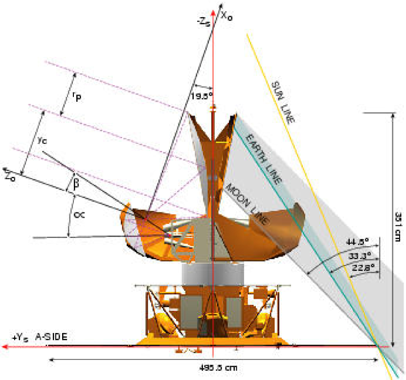
  Figure 1: Side view of the MAP optical system. The left side shows a cut-away view illustrating the relation of the microwave feeds to the optical system. We call the region around the feeds and secondary the optical cavity. The dashed lines represent three rays from a hypothetical feed at the center of the focal surface. The white conical structures are the feeds which are held in the FPA. The centrally located white gamma-alumina cylinder (diameter: 94 cm, height: 33 cm, thickness: 0.3 cm) thermally isolates the cold ($\approx 70~{}$K) optics from the warm ($\approx 290~{}$K) spacecraft. The parameters that describe a Gregorian are also shown. The right side shows how the Earth, Moon and Sun illuminate MAP at their minimum angles of incidence. In this view, the radiators are seen edge on. Platinum resistive thermometers are located on the primaries at $z_{s}=-350$ cm (top) and $z_{s}=-279$ cm (middle) and secondaries at $z_{s}=-214,-170,\&-138$ cm. Other views of the S/C may be found in Bennett et al. (2003), Jarosik et al. (2003), and Barnes et al. (2002).

1.2 Terminology and Conventions

Throughout this paper the following terminology is used: The thermal reflector system (TRS) consists of the primary and secondary mirrors of each telescope, the structure that supports them, and the passive thermal radiators as shown in Figure 1. The structure that holds the feeds and the cold end of the receiver chains is called the focal plane assembly, or FPA. The TRS fits over the FPA. A reflector evaluation unit (REU), which comprises half the TRS optics, was built to assess the design, for outdoor beam mapping, and as a ground reference unit. “S/C” is used for spacecraft.

In quantifying the MAP ’s response, where possible, the definitions of Kraus (1986) are used. The normalized antenna response to power is

$$B_{n}({\theta,\phi})={|\psi(\theta,\phi)|^{2}\over|\psi|^{2}_{max}},$$ (1)

where $\psi$ is the scalar electric field in units of ${\rm W^{1/2}m^{-1}}$ and is evaluated at a fixed distance from the source. The full-width-half-max of a symmetric beam is the angle at which $B_{n}(\theta_{fwhm}/2)=1/2$ (or $-3$ dB). When the beam is asymmetric, separate $\theta_{fwhm}$ are quoted or the geometric mean of the two $\theta_{fwhm}$ is used. At the output of any lossless antenna system, one measures the power in watts given by

$$W={1\over 2}\int_{\Omega}\int_{\nu}A_{e}(\nu)S_{\nu}(\theta,\phi)B_{n}({\nu,\theta,\phi})d\,\Omega d\,\nu,$$ (2)

where $A_{e}$ is the effective area of the antenna and $S_{\nu}(\theta,\phi)$ is the brightness of the sky. The directivity is

$$D_{max}\equiv{|\psi|_{max}^{2}\over|\psi_{avg}|^{2}}={4\pi|\psi|_{max}^{2}\over\int_{\Omega}|\psi(\theta,\phi)|^{2}d\Omega}=$$ (3)

$${4\pi\over\int B_{n}({\theta,\phi})d\Omega}={4\pi\over\Omega_{A}}={4\pi A_{e}\over n\lambda^{2}},$$

where $\Omega_{A}$ is the total solid angle of the normalized antenna pattern, $n$ is the number of radiative modes, and $|\psi_{avg}|^{2}$ is the total power averaged over the sphere. For single moded systems such as MAP, $n=1$. When there are no losses in the telescope, $G(\theta,\phi)=D_{max}\,B_{n}({\theta,\phi})$ and the directivity is the maximum gain.

The maximum gain, $G_{m}$, is sometimes just called the gain or “the gain above isotropic.” It can be understood by considering the flux (power/area) from an isotropic emitter of total power $P$. At a distance $r$, the flux is $P/4\pi r^{2}$ and the gain is unity (0 dBi). If instead the power were emitted by a feed of gain $G_{m}$ the flux at the maximum would be $I=G_{m}P/4\pi r^{2}~{}{\rm W/m^{2}}$. In other words, if one measures the field at a distance $r$ from the feed then

$$G(\theta,\phi)={4\pi r^{2}|\psi(r,\theta,\phi)|^{2}\over{\rm Total~{}emitted~{}power}}.$$ (4)

The absolute gain, as opposed to the relative gain, is important because it is the quantity that indicates one’s immunity to off-axis sources. If the gains for all MAP’s frequency bands were the same at some angle, each band would be equally susceptible to a source at that angle. The gain is always normalized so that

$$\int G(\theta,\phi)d\Omega/4\pi=\int_{S^{\prime}}{|\psi(x^{\prime},y^{\prime})|^{2}\over{\rm Total~{}emitted~{}power}}dx^{\prime}dy^{\prime}=1,$$ (5)

where the primed coordinates are for the aperture of the feed (or optical element).

The edge taper, $y_{e}$ is often useful in discussing the immunity of the optical system to sources in the sidelobes. In fact, from the value of the field at the edge of an optic, one can compute the approximate shape of the sidelobe pattern. The pattern is then normalized by the total power through the aperture. The edge taper is given in dB as $y_{e}=10\log(I_{edge}/I_{center})$ where $I$ is the intensity of the beam. For none of MAP’s bands is $y_{e}$ uniform around the edge; the largest (closest to $0~{}$dB) value is quoted.

2 Optical Design and Specification

In designing MAP , we considered a number of geometries including simple offset parabolas and three-reflector systems. In neither of these cases is the geometry of the feed placement conducive to having both inputs of a differential receiver view the sky. With the back-to-back dual reflector arrangement we have chosen, the feeds are centrally located and point in nearly opposite directions. Additionally, the S/C moment of inertia is minimized for a large optic.

There are a number of dual-reflector telescope designs Schroeder (1987); Love (1978). For radio work the Cassegrain (parabolic primary, hyperbolic secondary) and the Gregorian (parabolic primary, elliptical secondary) are often used . For some potential MAP geometries, the scanning properties of the Cassegrain system Ohm (1974); Rahmat-Samii & Galindo-Isreal (1981) were found superior to those of the Gregorian system. In other words, the beam pattern from a feed placed a fixed distance from the focus is more symmetric and has smaller near lobes. However, the offset Gregorian was chosen because the associated placement of the feeds was well suited to the differential receivers and the FPA could occupy the space made available by the position of the focus between the primary and secondary. Additionally, for a given beam size, the Gregorian is more compact than the Cassegrain Brown & Prata (1995).

Dragone (1986, 1988) developed extremely low sidelobe Gregorian systems in which the feed aperture is reimaged onto the primary. Such a system was used for the ACME CMB telescope Meinhold et al. (1992). Dragone’s work was used as a guideline but a number of factors complicated MAP ’s design: a) The feed apertures must be in roughly the same plane to avoid being viewed by one another. b) The feed inputs must cover ${\rm 20~{}cm\times 20~{}cm}$ to accommodate their large apertures. [The feed tails (receiver inputs) cover ${\rm 53~{}cm\times 53~{}cm}$ to make room for the microwave components; two W-band feed tails are separated by 19 cm; the two Ka-band feed tails are separated by 45 cm.] c) The secondary is in the near field of the feeds. For CMB telescopes, unlike the more familiar communications telescopes, beam efficiency is more important than aperture efficiency Rholfs (1986).

To understand the beams, accurate computer codes are essential. The baseline MAP design was done using code modified from the work of Sletten (1988) in which the far field beam pattern is computed from the square of the Fourier transform of the electric field distribution in the aperture. This simple and fast code combined with parametric models of the feeds and sidelobe response allowed rapid prototyping of various geometries while simultaneously optimizing over the combination of main beam size, contamination from the galactic pickup through the sidelobes, and the sidelobe level at the position of the Sun. All models followed the constraints for minimal cross-polar response Tanaka & Mizusawa (1975); Mizugutch et al. (1976). The parameters of resulting telescope are given in Table 1.

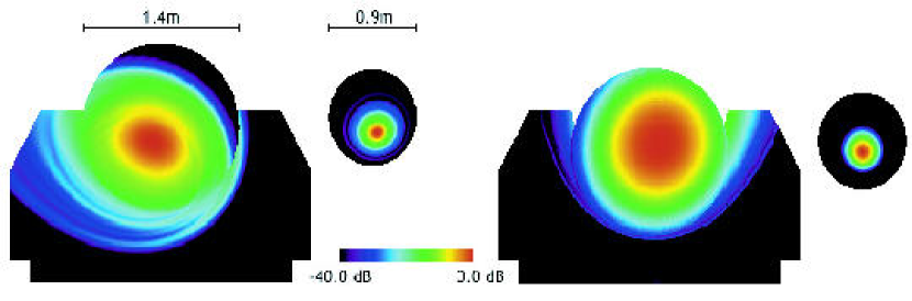
Figure 2: The current density on the primary and secondary reflectors for K-band (22 GHz) on the left and W-band (90 GHz) on the right. The 1.4 m diameter disk shows the projection of the primary as seen from the optical axis. The 2.7 m by 1.6 m rectangle with the modified corners shows the projection of the radiator panels. (The net emitting area of the panels is ${\rm 5.45~{}m^{2}}$.) As the far field approximates the square of the Fourier transform of the current density, one can see that the K-band beam will not be as symmetric as the W-band beam. The reflectors are in the near field of the telescope system so the apparent fraction of the beam spilled to the radiators is not indicative of the solid angle on the sky.

The DADRA “physical optics” computer code YRS Associates was used for the detailed design of MAP . From a spherical wave expansion of the field from a feed, the code determines the surface current on the secondary, ${\bf J}(r)=2\hat{\bf n}\times{\bf H}_{inc}(r)$. From this current, it computes the fields incident on the primary and thus the currents there. These currents are particularly useful for understanding the interaction of the optics with the S/C components. Examples are shown in Figure 2 for the lowest and highest frequency bands. The resulting beam is a sum of the fields from the feed and the currents on the primary and secondary reflector surfaces as shown in Figure 3. The method takes into account the vector nature of the fields and the exact geometry of the reflectors and the feeds. In principle, the currents can be unphysical near the reflector edges. In practice, because of the low edge taper, this approximation does not introduce significant errors. The code is excellent though its limitations are that a) only two reflections are considered, b) the possible interference of the feeds with the radiation from the reflectors and with each other is not accounted for, and c) the interactions with the structure are not accounted for. These interactions must be determined “by hand” and thus measurements of the assembled system are essential.

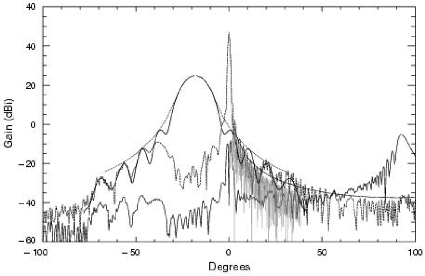
Figure 3: The optical response of a prototype design with a K-band feed at the focus of the telescope. The y-axis is the gain; the x-axis shows the angular distance from the primary optical axis. Negative numbers correspond to lines of sight below the optical axis as shown in Figure 1. The dashed line is the full model computed by the DADRA code for left circular polarization. The broad solid line that peaks at $-18\hbox{${}^{\circ}$}$ would be the response of the feed if it were not blocked by the secondary. Note that where the secondary does not intercept the feed pattern, $-40>\theta>15\hbox{${}^{\circ}$}$, the full pattern is dominated by the feed pattern. In other words, spill of the feed past the secondary dominates the optical response. The smooth dotted curve that envelopes the feed response is the parameterized model discussed in Section 2.3. The smooth line extending from the peak to $\theta=100\hbox{${}^{\circ}$}$ is the parameterized sidelobe response discussed in Section 2.7. The light curve for $0\hbox{${}^{\circ}$}<\theta<40\hbox{${}^{\circ}$}$ is from the aperture integration code. The curve that peaks at $\theta=90\hbox{${}^{\circ}$}$ is the response to radiation that has reflected once off the bottom of the secondary and into the feed and thus is right circularly polarized. This specific configuration was not built.

2.1 Flight Design

Once the baseline Gregorian design was set, the surfaces were “shaped” to optimize the symmetry and size of the beams YRS Associates ; Galindo-Isreal et al. (1992). The resulting reflectors differ from the pure Gregorian by $\approx~{}1~{}$cm in regions near the perimeter . For simple calculations, we use the best fit parameters shown in Table 1.

Table 1: Parameters of One Telescope

Quantity	Base Design	Best fit	Equiv parabola
Focal length, $f_{p}$ (cm)	90	90	206
Primary projected radius, $r_{p}$ (cm)	70	70	70
Offset parameter, $y_{c}$ (cm)	105	104.03	…
Interfocal distance, $2c$ (cm)	45	43.58	…
Secondary eccentricity, $e$	0.45	0.4215	…
$\beta$ (deg)	12.06	13.77	…
$\alpha$ (deg)	-31.12	-33.06	…

Cassegrain and Gregorian telescopes are defined by 5 parameters when they satisfy the minimum cross-polarization condition. These parameters are shown in Figure 1. Column 1 is the nominal conic design. Column 2 is the best fit to the shaped design with 5 free parameters. Column 3 shows the equivalent parabola Rausch (1990) for the best fit design described by the top five parameters. When the best fit design is constrained to follow the minimum cross-polarization condition, $\beta=14.32^{\circ}$ and $\alpha=-34.32^{\circ}$. The surface coating is vacuum deposited aluminum as discussed in section 2.8.

The shaped system does not have a sharp focus between the primary and secondary but one may still characterize its response in broad terms. The plate scale, how far one moves laterally in the focal plane to move a degree on the sky, for the shaped system is 4.44 cm/deg. This suggests an effective focal length of 250 cm, somewhat longer than that found from the equivalent parabola for the best fit model. The speed of the system, $f_{p}/D$ is f/1.8. The computer files containing the geometry are available upon request.

2.2 Manufacture and Alignment of Optics

The TRS and REU were built by Programmed Composites Inc. (PCI) to a specification Jackson et al. (1994). The structure that holds the optics is made of 5 cm by 5 cm “box beams” of 0.76 mm thick XN70/M46J composite material and has a mass of 23 kg. The reflectors are made of 0.025 cm thick XN70 spread fabric cloth face sheets over a 0.635 cm thick DuPont KOREX honeycomb core. The combination of materials was chosen based on PCI models that predicted a negligible net coefficient of thermal expansion between 70 and 300 K. The mass of one primary, with the backing structure, is 5 kg. The mass of one secondary is 1.54 kg. The radiator panels are made of 1100 series H14 aluminum over a 5.08 cm aluminum honeycomb core and each has a mass of 8 kg. They are painted with NS43G/Hincom white paint to minimize their solar absorptance, ensure a conducting surface, and maximize their infrared emissivity. The full TRS, with harnesses and thermal blankets, has a mass of 70 kg.

The specifications were set to meet the science goals and to easily mesh with known tolerances in the manufacturing process to keep costs down. The surface rms deviation at 70 K from the ideal shape over the whole reflector was specified to be $<0.0076~{}$cm or $\approx\lambda/40$, and is discussed in more detail below. The reflectors, when treated as rigid bodies satisfying the surface rms criteria and when positioned on the TRS structure and cooled to 70K, were specified to be within 0.038 cm of the design position. This specification includes all rotations and translations and accounts for the effects of moisture desorption, gravity relief, and cooldown from room temperature. The on-orbit predictions are given in Table 2.

Table 2: S/C Coordinates for A-side

Object	$x_{s}$ (cm)	$y_{s}$ (cm)	$z_{s}$ (cm)
Focus	0	65.0	-166.0
Top of A Primary	0.045	35.99	-351.66
Bottom of A Primary	0.040	7.58	-192.75
$+x$ Boundary of A Primary	70.05	21.77	-272.30
Top of A Secondary	0.031	123.31	-215.85
Bottom of A Secondary	-0.011	102.20	-136.00
$+x$ Boundary of A Secondary	39.12	36.73	-176.36

The optics were built to have no adjustments. They were designed to be in focus at 70 K and so were deliberately though insignificantly out of focus for all testing at 290 K. A full STOP (Structural Thermal OPtical) performance analysis of the optical design was performed using the W-band beam pattern because it is the most sensitive to changes in the position. The analysis includes changes in the position and orientation of the optics and feeds as they cool. The worst case displacements upon cooling lead to a $0.1^{\circ}$ shift in beam elevation and a $0.14^{\circ}$ shift in azimuth, dominated by orientation changes in the primary. These are not significant from a radiometric point of view. In addition, all final pointing and beam information is determined from in-flight observations. Table 3 shows the placement of the feeds along with the predicted beam positions on the sky. Tables 1, 2 and 3 completely specify the geometry for the conic approximation.

In addition to the usual metrology tools, photogrammetry and laser tracking were found to be particularly useful. Photogrammetry was used to determine the change in the shape of the optics upon cooling to 70 K. The laser tracker allowed the rapid digitization of thousands of points on the reflectors which was useful for surface fitting and measuring the surface deformations.

Table 3: Design Positions of Main Beams

Beam	Aperture	OMT to Apt vector	Direction on sky	P1	P2
K1A	(9.49,73.21,-177.06)	(-0.2303,0.9438,0.2370)	(0.0404, 0.9246, -0.3788)	(0.6927, -0.2991, -0.6562)	(-0.7200,-0.2358,-0.6526)
K1B	(9.47,-73.26,-177.08)	(-0.2301,-0.9438,0.2372)	(0.0407,-0.9240, -0.3803)	(0.6951,0.2996,-0.6535)	(-0.7178,0.2377,-0.6545)
Ka1A	(-8.66,73.35,-176.24)	(0.2438,0.9367,0.2515)	(-0.0377, 0.9258, -0.3762)	(-0.6964, -0.2943, -0.6545)	(0.7167, -0.2373, -0.6558)
Ka1B	(-8.64,-73.42,-176.24)	(0.2434,-0.9371,0.2501)	(-0.0374, -0.9251, -0.3778)	(-0.6938, 0.2961,-0.6564)	(0.7191, 0.2376, -0.6530)
Q1A	(-7.20,71.93,-158.79)	(0.2146,0.9527,-0.2152)	(-0.0314, 0.9523, -0.3034)	(0.7119, -0.1918, -0.6756)	(-0.7015, -0.2373, -0.6720)
Q1B	(7.19,-71.99,-158.78)	(0.2155,-0.9524,-0.2155)	(-0.0319, -0.9522,-0.3037)	(0.7147, 0.1907, -0.6729)	(-0.6987, 0.2385, -0.6745)
Q2A	(7.20,71.93,-158.79)	(-0.2150,0.9527,-0.2148)	(0.0328, 0.9523, -0.3034)	(-0.7147, -0.1899, -0.6731)	(0.6986, -0.2389, -0.6744)
Q2B	(7.19,-71.98,-158.77)	(-0.2153,-0.9523,-0.2161)	(0.0323, -0.9522, -0.3037)	(-0.7121, 0.1912, -0.6755)	(0.7013, 0.2381, -0.6719)
V1A	(-8.00,71.00,-167.40)	(0.2076,0.9782,0.0082)	(-0.0328, 0.9416, -0.3352)	(-0.6976, -0.2617, -0.6669)	(0.7157, -0.2119, -0.6659)
V1B	(-7.93,-71.07,-167.37)	(0.2072,-0.9783,0.0071)	(-0.0333, -0.9415, -0.3354)	(-0.6994, 0.2617, -0.6651)	(0.7140, 0.2125, -0.6672)
V2A	(8.00,71.00,-167.40)	(-0.2077,0.9782,0.0076)	(0.0335, 0.9416, -0.3352)	(0.6986, -0.2620, -0.6660)	(-0.7149, -0.2118, -0.6664)
V2B	(7.92,-71.07,-167.37)	(-0.2073,-0.9783,0.0071)	(0.0331, -0.9415, -0.3354)	(0.6974, 0.2621, -0.6670)	(-0.7160, 0.2119, -0.6652)
W1A	(-2.40,70.02,-170.00)	(0.0432,0.9978,0.0501)	(-0.0087, 0.9396, -0.3422)	(0.7098, -0.2352, -0.6639)	(-0.7043, -0.2487, -0.6649)
W1B	(-2.40,-70.15,-170.03)	(0.0428,-0.9979,0.0496)	(-0.0095, -0.9394, -0.3428)	(0.7100, 0.2351, -0.6638)	(-0.7041, 0.2497, -0.6647)
W2A	(-2.40,69.98,-165.20)	(0.0364,0.9989,-0.0290)	(-0.0091, 0.9459, -0.3245)	(-0.7058, -0.2359, -0.6679)	(0.7083, -0.2229, -0.6697)
W2B	(-2.46,-70.11,-165.21)	(0.0356,-0.9989,-0.0302)	(-0.0095, -0.9458, -0.3247)	(-0.7056, 0.2365, -0.6680)	(0.7085, 0.2228, -0.6696)
W3A	(2.40,69.98,-165.20)	(-0.0351,0.9990,-0.0289)	(0.0101, 0.9457, -0.3248)	(0.7058, -0.2368, -0.6677)	(-0.7083, -0.2225, -0.6699)
W3B	(2.45,-70.08,-165.19)	(-0.0368,-0.9989,-0.0296)	(0.0093, -0.9458, -0.3247)	(0.7049, 0.2365, -0.6687)	(-0.7092, 0.2227, -0.6689)
W4A	(2.40,70.02,-170.00)	(-0.0428,0.9978,0.0500)	(0.0101, 0.9394, -0.3426)	(-0.7095, -0.2347, -0.6645)	(0.7046, -0.2498, -0.6642)
W4B	(2.39,-70.18,-170.02)	(-0.0436,-0.9978,0.0496)	(0.0093, -0.9394, -0.3428)	(-0.7102, 0.2351, -0.6636)	(0.7039, 0.2497, -0.6650)

These values and unit vectors are in S/C coordinates and thus can be directly compared to Table 2. The final beam position will be determined in flight. The “aperture” is the coordinate in the focal plane. “OMT to Apt” is the unit vector along the symmetry axis of the feed. “Direction on sky” is the unit vector along the optical axis. The polarization directions, P1 and P2, correspond to the maximum electric field for the main (or axial) and side (or radial) OMT ports respectively. The “1” or “2” is the last number in a radiometer designation. A DA differences two polarizations of similar orientation on the sky as can be seen by comparing K11A, polarization direction 1 (P1) on the A side, and K11B, the matching input to the DA on the B side.

2.3 Feeds

The inputs of the differential microwave receivers are coupled to free space with corrugated microwave feeds Barnes et al. (2002). The initial designs followed well known principles Thomas (1978); Clarricoats & Olver (1984) though the final groove dimensions were optimized YRS Associates . Corrugated feeds were chosen because a) their patterns are accurately computable and symmetric; b) they have low loss; and c) they have low slidelobes. Table 4 summarizes the features of the MAP feeds.

At the base of each feed is an orthomode transducer (OMT), the microwave analog of a polarizing beam splitter. The two rectangular waveguide outputs of the OMT, the “main” port and the “side” port, carry the two constituent polarizations to the inputs of separate differencing assemblies Jarosik et al. (2003). As the polarization cannot be determined in flight, it is completely characterized on the ground.

The beam from each feed is diffraction limited so that the illumination patterns on the secondary and primary are a function of frequency. Because the secondaries are in the near field of the feeds, $d<2d_{fapt}^{2}/\lambda$, the phase center concept is not useful for detailed predictions. A full electromagnetic code such as CCRHRN YRS Associates is essential. However, for the top level parameterization of MAP the feeds were modeled as open corrugated wave guides with $B_{n}(\theta)=[x_{1}^{2}J_{0}(v)/(x_{1}^{2}-v^{2})]^{2}$ where $v=kr_{1}\sin(\theta)$, $x_{1}\approx 2.405$, $k=2\pi/\lambda$, and $r_{1}$ is the radius of the waveguide Clarricoats & Olver (1984). At large angles, the envelope $J_{0}(v)\approx\sqrt{2/v\pi}$ is shown in Figure 3 for a K-band feed.

Table 4: Feeds and OMTs

Band	K	Ka	Q	V	W
Center frequency (GHz)	23	33	41	61	93
$\theta_{FWHM}^{\rm feed}$ (deg)	$8.8^{\circ}$	$8.3^{\circ}$	$7.0^{\circ}$	$8.0^{\circ}$	$8.4^{\circ}$
$G_{m}^{\rm feed}$ (dBi)	26.79	27.23	28.77	27.28	26.40
$d_{fapt}$ (cm)	10.94	8.99	8.99	5.99	3.99
$Crosspol^{omt}$ (dB)	-40	-30	-30	-27	-25

See also Jarosik et al. 2003. The maximum gain, $G_{m}$, is for a lossless feed.

2.4 Main Beams

The main beam width is determined by the size of the primary mirror, the edge taper (Table 7) and to a lesser degree, the beam profiling. As discussed in Section 2.7, the edge taper is $\approx-20~{}$dB, except in K-band. With a 1.4 m projected primary diameter, the beam width is $\theta_{fwhm}\approx 0.5^{\circ}(40~{}{\rm GHz}/\nu)$. Because a diffraction limited feed illuminates the primaries and secondaries with a low edge taper, the beam width is a relatively weak function of frequency within a frequency band as shown in Table 5.

The number of feeds and radiometers in each frequency band is chosen so that each band has roughly equal sensitivity per unit solid angle to celestial microwave radiation. Because the noise temperature of HEMT amplifiers scales approximately with frequency Pospieszalski (1995), MAP has 1 feed in K-band and Ka-band, 2 feeds in Q-band and V-band, and 4 in W-band.

The desire for broad frequency coverage and multiple channels requires the maximal use of the telescope focal plane. The layout of the two back-to-back telescopes shown in Figure 1, and the need for a compact enclosure for all the differential radiometers places difficult constraints on the geometry of the feeds, the radiometers, and the focal-plane arrangement. In particular, the need for roughly equal total feed length, the requirement for minimum cross-talk and obscuration between feeds in the focal plane, and the placement of the OMTs and cold amplifiers lead to feed-telescope solutions which required evaluation with full diffraction calculations for optimizing the configuration. For example, the K-band feed is profiled to reduce its length by a factor of $\approx 50$% from its nominal geometry. The K-band feed is also shifted along its axis by 15 cm toward the secondary from its optimal position. Such large departures from usual practices are acceptable if the design can be evaluated and the beam profiles and solid angles can be measured to $\approx 0.5$% accuracy in flight.

In general, a controlled loss of axial symmetry of the beam point spread function was balanced against other geometrical constraints as the whole system was considered simultaneously. The solution for the reflectors results in an uninverted image of the sky on a slightly curved focal plane. The geometric image quality degrades with increasing distance from the optics axis. Within a $2^{\circ}$ diameter centered on the optical axis, 95% of the incident power falls within a 0.4 cm diameter disk. Further out, within a $4^{\circ}$ diameter region the 95% disk is 1 cm in diameter.

Table 5: Predicted ideal K-band and W-band main beams

K-band Frequency (GHz)	20	22	25
Feed 3 dB width (deg)	10.0	8.9	7.7	$\dots$
Vertical 3 dB width (deg)	0.969	0.882	0.787	$\dots$
Horizontal 3 dB width (deg)	0.798	0.721	0.637	$\dots$
$G_{m}$ (dBi)	46.30	46.97	47.79	$\dots$
$\Omega_{A}$ (sr)	$2.82\times 10^{-4}$	$2.44\times 10^{-4}$	$2.03\times 10^{-4}$	$\dots$
$\sqrt{\Omega}/\lambda$ (cm-1)	0.0112	0.0115	0.0119	$\dots$
$A_{eff}$ (m2)	0.80	0.76	0.71	$\dots$
Primary edge taper (dB)	$-12.8$	$-13.1$	$-14.7$	$\dots$
W-band Frequency (GHz)	82	90	98	106
Feed 3 dB widtha (deg)	27.9	25.0	$\dots$	21.4
$+45^{\circ}$ slice 3 dB beam width (deg)	0.209	0.201	0.198	0.194
$-45^{\circ}$ slice 3 dB beam width (deg)	0.199	0.190	0.184	0.181
$G_{m}$ (dBi)	59.40	59.75	59.95	60.09
$\Omega_{A}$ (sr)	$1.43\times 10^{-5}$	$1.33\times 10^{-5}$	$1.27\times 10^{-5}$	$1.23\times 10^{-5}$
$\sqrt{\Omega}/\lambda$ (cm-1)	0.0103	0.0109	0.0116	0.0124
$A_{eff}$ (m2)	0.94	0.83	0.74	0.65
Primary edge taper (dB)	$-17.4$	$-21.0$	$-24.8$	$-26.5$

2.5 Polarization

The optical system is designed to minimize the cross-polarization. The OMTs attached to the azimuthally symmetric feed defines the polarization direction. Each OMT is oriented so that the polarization directions accepted by the feeds are $\pm 45^{\circ}$ with respect to the $yz$ symmetry plane of the satellite. The unit direction vectors on the sky are given in Table 3. The $45^{\circ}$ angle ensures that the two linear polarizations in one feed nearly symmetrically illuminate the primary and secondary. Consequently, the beam patterns for both polarizations are nearly identical.

There are some subtleties in specifying the polarization angle. For example, the average of the polarization angle within a $-3$ dB contour of the main beam does not equal the polarization direction at the beam maximum. It can differ by of order a degree. MAP’s angles were set to $\pm 45^{\circ}$ at the beam maximum. Even though the corresponding orientation of the OMT was found using the full diffraction calculation, the same orientation is obtained with purely geometrically considerations.

The MAP polarization angle was measured in the NASA/GSFC beam mapping facility. A polarized source was rotated to minimize the average signal across all frequencies in the band. The polarization angle was then taken to be $90^{\circ}$ from that angle. The measured polarization minimum does not occur at the same angle across the band and so a best overall minimum angle was approximated. The uncertainty of the radiometric measurement is $\pm 1^{\circ}$. Across all bands and all feeds, the scatter in polarization angle is $\pm 2^{\circ}$. The uncertainty in the polarization angle based on the metrology of the OMT orientation is $\pm 0.2^{\circ}$. We use $\pm 1^{\circ}$ as the formal error. The resulting maximum misidentification of power due to the rotational alignment uncertainty is $\approx 1-\cos^{2}(1^{\circ})\approx 0.0003$.

The cross-polar leakage is not zero but is sufficiently small to allow the measurement of the CMB polarization to the limits of the detector noise. In K and Ka bands, the cross polar contribution to the co-polar beam is $-25$ dB and $-27$ dB respectively, and is dominated by the reflector geometry in combination with the feed placement. In Q, V, and W bands, the cross-polar contributions to the co-polar response are $-24$ dB , $-25$ dB, and $-22$ dB respectively and arise from a combination of imperfect OMTs, as shown in Table 4, and reflector geometry.

2.6 Surface Shape

The smoothness of the optical surface and the placement of the feeds determine the quality of the beams. The measured beam profiles, especially in W-band, do not precisely match the predictions for ideal reflectors. However, they are in excellent agreement with the computations based on the measured distortions of the reflector surfaces.

The characteristics of the profiles are also in good agreement with the Ruze (1966) model which accounts for the axial loss of gain and the pattern degradation as a function of the reflector surface rms error, $\sigma_{z}$, and the spatial correlation length of the distortions, $l_{c}$. For lossless Gaussian shaped distortions, which sufficiently describe the surfaces,

$$G(\theta,\phi)=G_{0}(\theta,\phi)e^{-\overline{\rho^{2}}}+$$

$$\left(\frac{2\pi l_{c}}{\lambda}\right)^{2}e^{-\overline{\rho^{2}}}\sum_{n=1}^{\infty}\frac{\overline{\rho^{2}}^{n}}{n\times n!}e^{-\left(\pi l_{c}\sin(\theta)/\lambda\right)^{2}/n}$$ (6)

where $\lambda$ is the wavelength, $G_{0}(\theta,\phi)$ is the ideal undistorted prediction, $\overline{\rho^{2}}$ is the variance of the phase error, equal to $k^{2}{\sigma_{z}}^{2}$, and $l_{c}$ is the correlation length. The number of distorted “lumps,” $\approx(D/2l_{c})^{2}\approx 50$, is large enough to satisfy the statistical assumptions behind Ruze’s model.

The first term in equation 6 shows that the reduction in forward gain from the undistorted reflector is determined by $\sigma_{z}$ and is independent of $l_{c}$. The second term, the “Ruze pattern,” is a function of $\theta$, is independent of the undistorted pattern, and is determined by $l_{c}$ and $\overline{\rho^{2}}$. The shoulder of the Ruze beam is mostly determined by $l_{c}$. Increasing the $\sigma_{z}$ from zero while keeping $l_{c}$ constant lowers the forward gain and raises the Ruze beam, without changing the shoulder. Increasing $l_{c}$ from zero narrows the Ruze pattern.

The surface shape was specified to achieve close to ideal performance. Ground testing revealed that the primary mirror shape met the specification at room temperature but would not at the second Earth-Sun Lagrange point , L₂, from where MAP observes Bennett et al. (2003). At room temperature, the surface parameters are computed from measurements of the surface made with a laser tracker. The cold shape of the surface was determined through photogrammetry of 35 targets affixed to a 90 K primary and then extrapolated to 70 K, the prediction for L₂. The results are given in Table 6. The departure from the ideal shape is rooted in errors in the estimates of the thermal coefficients of expansion of some of the materials. Even though the diameter of the secondary is two thirds that of the primary, it is less susceptible to cool-down distortions. This is attributed to its cylindrically symmetric mount and more extensive backing structure as opposed to the “goal post” mount for the primaries.

Table 6: Reflector Surface Shape Parameters

Reflector	Spec $\sigma_{z}$	$\sigma^{290K}_{z}$ (cm)	$\sigma_{z}^{70~{}K}$ (cm)	$l_{c}$ (cm)	$e^{-\overline{\rho^{2}}}$ warm	$e^{-\overline{\rho^{2}}}$ cold	$kl_{c}$
Primary P3 (A side)	0.0076	0.0071	0.023	9.3	0.989	0.826	175
Primary P2R (B side)	0.0076	0.0071	0.024	11.4	0.987	0.812	213
Secondary S4 (A side)	0.0076	0.0071	$\cdots$	10.1	0.988	$\cdots$	191
Secondary S5 (B side)	0.0076	0.0076	$\cdots$	9.7	0.991	$\cdots$	183

An approximation is made to compute the gain of the primary beam pattern for the full telescope. First, $G_{p}$ is computed by substituting $l_{c}$, $\overline{\rho^{2}}$, and the ideal $G_{0}$ into equation 6. Next $G_{p}$ is substituted for $G_{0}$ in Ruze’s formula, with $l_{c}$ and $\overline{\rho^{2}}$ for the secondary. The final result is this newly determined $G(\theta)$. It is compared to the azimuthally averaged gain of the model. This method ignores the fact that the primary is in the near field of the secondary. Results are plotted for the warm reflectors in Figure 4 along with measurements and predictions from the DADRA code. For the warm reflectors, the simple model reproduces the overall shape but misses the lobe at $\theta=0.45^{\circ}$.

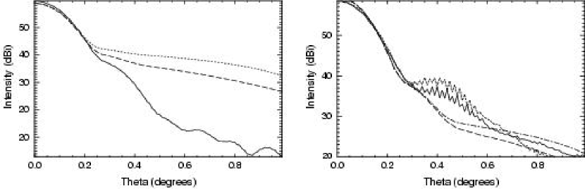
Figure 4: Left: Beam profiles at 90 GHz from a distorted surface based on Gaussian deformations (dashed line, eq. 6) and hat box distortion (dash-dot line, Ruze (1966)). The azimuthally averaged measured warm profile (solid line) is shown with the DADRA predictions based on the measured distorted surface (dotted line). Right: Predictions for the cold optics based on the values in Table 6 for Gaussian distortions (dashed line), hat box distortions (dotted line), and the undistorted mirror (solid line). At $\approx 2^{\circ}$ all curves meet.

For the on-orbit predictions, the same procedure is followed except that the cold $\sigma_{z}$ is used. We assume that the correlation length does not change. The results are plotted in Figure 4. The Ruze beam dominates the undistorted beam for $0\fdg 2<\theta<2^{\circ}$, and above $2^{\circ}$ is subdominant to it, diminished by the exponential factor. Even $1\fdg 4$ from the boresight, the Ruze beam is $<-35~{}$dB below the peak. The full W-band patterns for the ideal and distorted beams are plotted in Figure 5.

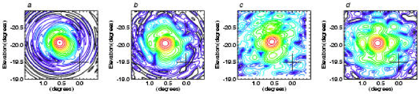
Figure 5: A comparison of the W4A beams at 90 GHz. The panels show: (a) predictions for an ideal-mirror beam pattern, (b) predictions for an ambient temperature distorted mirror beam pattern, (c) the measured beam pattern, and (d) the prediction for a cooled mirror in orbit. The contour intervals are 3 dB. The cross indicates the center of the focal surface.

An additional potential source of degradation of the main beams is print through of the weave pattern that comprises the fabric that makes up the surface of the reflectors. This was investigated by measuring the change in the holographic pattern of a sample surface upon cooling Jackson & Halpern . For a 200 K change, the contrast of the weave increases from 0 to $\approx 2~{}\mu$m. From this pattern, one computes an upper bound of -70 dB in W-band for a narrow sidelobe $40\hbox{${}^{\circ}$}$ off the main beam. Contributions from bright sources, for example Jupiter, through this lobe will be $<0.1~{}\mu$K.

2.7 Sidelobes

The sidelobes are small, well characterized, theoretically understood, and measured. Generally, sidelobes are produced by illumination of the edges of the optical elements whereas the main beam profile is determined by the shape of the elements. The primary radiometric contamination comes from hot sources, such as the Earth, Moon, and Sun (Table 9), well outside the main beam. Also, contamination arises from the Galaxy, which is much colder, $\approx 200~{}$mK, but is extended and closer to the main beam. For scale, if the Sun is to contribute less than $2~{}\mu$K to any pixel, it must be rejected at $(2~{}\mu{\rm K}/T_{Sun})(\Omega_{Sun}/\Omega_{A})\approx-100~{}$dB.

The six principal contributions to the sidelobes are: a) response of the feeds to radiation outside the angle subtended by the subreflector; b) diffraction from the edge of the secondary; c) diffraction from the edge of the primary; d) spill past the edge of the primary; e) scattering from the structure that holds the feeds; and f) reflection off the radiators by radiation that goes past the primary. The more negative the edge taper, the smaller each of these is.

The sidelobe levels are computed in two ways. For the contributions from the radiators and optical surfaces, the full physical optics calculation is used YRS Associates . The commercial code was rewritten to take into account the interaction of the radiators with the primary mirrors. As the Sun, Earth, and Moon are shielded by the 5 m diameter solar shield, which is not part of the physical optics model, the geometric theory of diffraction [GTD, Keller (1962)] is used to compute their contribution.

In GTD, the field diffracted by an edge is given by $\psi_{s}(r)=D_{GTD}\psi_{i}(r(1+r/\rho_{1}))^{-1/2}e^{ikr}$, where $\psi_{i}$ is the incident field (or field at the edge), $r$ is the distance to the edge, $\rho_{1}$ is a radius of curvature that characterizes the edgeKeller , and the diffraction coefficient $D_{GTD}$ is

$$D_{GTD}=-{e^{i\pi/4}\over 2\sqrt{2\pi k}}\biggl{[}{1\over\cos((\phi-\alpha)/2)}\pm{1\over\sin((\phi+\alpha)/2)}\biggr{]}.$$ (7)

For a straight edge $1/\rho_{1}=0$ and one recovers Sommerfeld’s solution. The angles are shown in Figure 6. The upper sign is for the incident E-field perpendicular to edge and the lower sign is for the E-field is parallel to the edge.

Radiation from the Sun diffracts around the edge of the solar shield, diffracts over the top of the secondary, and then enters the feeds as can be seen in Figure 1. Radiation from the Earth and Moon diffracts directly over the top of the secondary and then enters into the feeds. To compute these contributions, the rim of the solar shield is approximated as straight (outboard of the secondary it is almost straight). The edge of the secondary is approximated with a radius of curvature of $r_{s}=40~{}$cm so that $1/\rho_{1}=-\cos(3\pi/2-\phi)/r_{s}$. For all estimates, the phase in equation 7 is ignored.

Consider first the contribution from the Earth with temperature $T_{E}$ and solid angle $\Omega_{E}$. The antenna temperature is given by

$$T_{A}={|D_{GTD}|^{2}\over r}{G(\theta_{edge})\over 4\pi}T_{E}\Omega_{E},$$ (8)

where $G(\theta_{edge})$ is the gain of the feed at the edge of the secondary, $r$ is the distance to the secondary, and $D_{GTD}$ is given by equation 7 with the geometry in Figure 1. The diffraction effects are greatest for K band because it has the largest wavelength so only it is considered. Using the parameters in Table 9 and $G(\theta_{edge})=-22.4~{}$dBi, $\alpha=-76^{\circ}$, $\phi=200^{\circ}$, and $r=60~{}$cm, one finds $D_{GTD}=0.36~{}$cm^1/2 and $T_{A}\approx 60~{}$nK. Similar calculations for the Moon yield $T_{A}\approx 4~{}$nK and for the Sun, after taking into account the double diffraction, $T_{A}\approx 16~{}$nK.

=7cmf6j.ps

Fig. 6. The geometry for the diffraction calculations. On the left, the incident and reflected rays are measured with respect to a line perpendicular to the screen (viewed edge on). On the right is a disk, for example the primary. The dot-dashed lines are the two scattered rays from the edge.

Similar order-of-magnitude calculations were used to check multiple diffraction paths and angles. It was found that solar radiation could directly enter the feeds by diffracting from the $\pm x$ edges of the secondary and the truss structure that holds the secondary. As a result, additional “diffraction shields” were added that go between the front of the structure that holds the feeds (FPA) and the edge of the secondary to eliminate these paths.

GTD was also used early in the design phase in the parametric model of the satellite (Section 2). The illumination of the primary for the field $\psi$ was modeled as a Gaussian of width $\sqrt{2}\sigma_{p}$ with edge taper $y_{e}$ so that

$$\exp(-r_{p}^{2}/4\sigma_{p}^{2})=10^{y_{e}/20}<<1$$ (9)

at the rim of the primary, $r=r_{p}$. For a circular disk or aperture evaluated in the limit of $r>>r_{p}$ and intermediate angles

$$\psi_{s}(r,\theta)=D_{GTD}\psi_{i}(r^{2}\sin\theta/r_{p})^{-1/2}e^{ikr},$$ (10)

and

$$D_{GTD}=-{1\over 2\sqrt{2\pi k}}\biggl{[}{1\over\sin(\theta/2)}\pm{1\over\cos(\theta/2)}\biggr{]}$$ (11)

At large angles, diffraction with E parallel to the edge dominates and the full expression becomes

$$G(\theta)={4\pi r^{2}\psi_{s}^{2}(r,\theta)\over{\rm Total~{}power}}\approx$$

$${\ln(10^{1/20})|y_{e}|10^{y_{e}/10}\over\pi r_{p}k}{1\over\sin\theta}\biggl{[}{1\over\sin(\theta/2)}+{1\over\cos(\theta/2)}\biggr{]}^{2}$$ (12)

A curve of equation 12 is shown in Figure 3.

Because of the large uncertainty associated with the hand GTD calculations and the need to confirm the computer models, the sidelobes were measured in K, Q, and W bands using a full-scale replica of the satellite built around the REU. The results from the full diffraction calculation for K band along with measurements at the same frequency are shown in Figure 7.

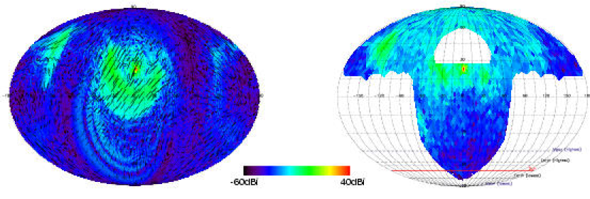
Figure 7: Left: Predicted sidelobe response at 22 GHz over the full sky. The main beam is shown at an elevation of $17^{\circ}$. The forward gain is 47 dBi and so is suppressed on this plot by almost $10^{5}$. The arrows indicate the polarization direction. The large lobe in the upper left side is from spill past the place where the primary and radiator meet on the left hand side of Figure 2. The large rings are from diffraction around the secondary. The lobe in the upper right is from reflection off the radiator just below where the lobe on the left passes through. Note that the most prominent lobe is polarized. Also, K band has, by far, the largest sidelobes. This calculation does not include any effects from the solar array panel. Right: Measurement of the sidelobes at the same frequency but with the FPA and solar array in place. The hole in the upper central part is from incomplete coverage. The gross features agree. The extra power in the central upper hemisphere, as compared to the prediction, is from scattering off the top of the FPA. Because it is diffuse and at a low level, $\approx-30~{}$dBi, it is not a significant source of pickup. The solar array blocks all radiation in the lower hemisphere.

2.7.1 Radiometric Contributions From Sidelobes

To assess the contribution to the radiometric signal from Galactic emission, the full sky differential beam maps were “flown” over a galactic template. The beam maps were made from a composite of the computer model and the measurements. The galactic template is based on the Haslam and IRAS maps scaled to be $T_{gal}=230,100,70,40,50~{}$mK in K through W bands respectively in a $4\times 10^{-6}$ sr pixel at $l=0,b=0$.

The A-side beam is placed in each pixel of the map and the negative B-side beam is rotated through $360^{\circ}$ in $10^{\circ}$ intervals. The contributions for $G>15~{}$dBi are excluded as these are right next to the main beam and will naturally be incorporated into the map solution. (For V and W band this corresponds to one pixel.) At each orientation, the following integration is performed:

$$T_{A}={1\over 4\pi}\int G(\theta,\phi)T_{gal}(\theta,\phi)d\Omega$$ (13)

where $G(\theta,\phi)$ is the telescope gain. For each ring, the minimum, maximum, and rms signals are recorded. Data with the B-side beam at $|b|<15^{\circ}$ are excluded. The results are given in Table 7.

Verifying the GTD calculations entails a measurement of the sidelobes at the -70 dBi level. Measurements using the test range between the roof tops of Princeton’s physics and math buildings are limited by scattering at the -50 dBi level, 110 dB below the peak in W-band, even after covering large areas of ground with microwave absorber. Consequently, only an upper limit of $0.5~{}\mu$K may be placed on contamination by the Sun, Earth, and Moon.

Table 7: Contributions and Parameterization of the Sidelobe response

Band designation	K	${\rm K_{a}}$	Q	V	W
Center frequency (GHz)	23	33	41	61	93
Maximum ($\mu$K)	$85$	$10$	$20$	$2$	$1.5$
Minimum ($\mu$K)	$-150$	$-60$	$-40$	$-3$	$-5$
rms ($\mu$K)	$12$	$2$	$3$	$0.2$	$<0.1$
Max. Edge taper (dB)	-13	-20	-21	-21	-16/-20
Forward beam efficiency	0.960	0.986	0.986	0.996	0.996/0.999

2.8 Reflector Surfaces

Coatings were applied to the optics to provide a surface a) whose microwave properties are essentially indistinguishable from those of bulk aluminum, b) that radiates in the infrared so that the reflector does not heat up unacceptably when the Sun strikes it, c) that diffuses visible solar radiation so that sunlight is not focused on the focal plane or the secondary, and d) that does not allow the build up of excessive amounts of charge in orbit. These four criteria can be met simultaneously Heaney et al. (2001).

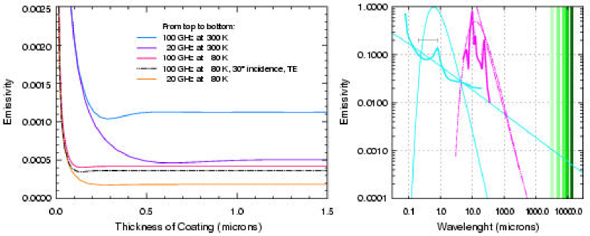
Figure 8: Left: The theoretical emissivity of a thin aluminum coating as a function of the thickness of the coating. The dip in the curve is an interference phenomenon (Born & Wolf pg. 628). At small coating thicknesses, the results differ from those in Xu et al. (1996) and give a somewhat smaller thickness at the minimum than Garg et al. (1975) who find $t/\delta\approx\pi/2$, where $\delta$ is the skin depth. The variation in emissivity with incident angle is not significant. The dot-dot-dot-dash line is for the TE mode (E perpendicular to plane of incidence) with a $30^{\circ}$ incident angle. The TM mode will be higher than the nominal value. The effects of the composite substrate are negligible (e.g., Ramo & Whinnery pg 249). Right: The emissivity of the surface from optical to microwave wavelengths. The aluminum emissivity is based on the Drude model (solid straight line, e.g., Ashcroft & Mermin (1976)) and measurements (curve with a peak at $1~{}\mu$m). The visible band is indicated by a bar at an emissivity of $e=0.2$, just below the peak of a 6000 K blackbody representing the Sun. The jagged line at 10 $\mu$m is the emissivity of ${\rm SiO_{2}}$ and the dot-dot-dot-dash line is a model of its long wavelength behavior. The vertical bands on the right are the MAP bands

The coating is vacuum deposited onto a surface comprised of an $\approx 25~{}\mu$m thick layer of epoxy over a 250 $\mu$m composite sheet. The epoxy layer is roughened to diffuse sunlight and not affect the microwave properties, and is then coated with aluminum and SiO_x (the “$x$” denotes unknown, as the material is a combination of SiO and SiO₂). The SiO_x coating, because of an absorptance resonance, allows the reflector to radiate at $10~{}\mu$m, near the peak of a 300 K blackbody, as shown in Figure 8. To maximize the infrared radiation, thicker SiO_x is better, but if the layer exceeds $2.5~{}\mu$m it insulates the aluminum unacceptably leading to potential problems with surface charging in space.

Obtaining a successful coating was particularly challenging . The mission requirement that the optics be able to withstand transient direct illumination by the Sun was a significant complication. To maintain high surface quality, especially in the micron wavelength region, the flight reflectors were maintained at $<50$% relative humidity from when they were coated until launch.

2.8.1 Roughening the Surface

The reflector surfaces are roughened to diffuse the solar radiation so that the secondaries and feeds do not get too hot from the focused radiation from the primary. The specification, which is developed below, is that no more than 20% of the reflected radiation be inside the $20^{\circ}$ (full angle) cone of the reflected ray at a wavelength of 540 nm. Measurements show this is possible if the surface has a $0.4~{}\mu$m roughness with a correlation length of $30~{}\mu$m, in agreement with the models Bennett & Porteus (1961).

Reflection from a roughened surface is quantified with the bidirectional reflectance (BDR), $\rho^{\prime}$, and $\rho_{d}$, the directional reflectance (DR) Nicodemus (1965); Beckmann & Spizzichino (1963); Davies (1954); Houchens & Hering (1967). The BDR is the reflection coefficient per unit solid angle for arbitrary incident polar directions ($\psi,\zeta$) and reflection directions ($\theta$,$\phi$) measured from the mean normal of the surface:

$$\rho^{\prime}(\psi,\zeta;\theta,\phi)\equiv{\delta I_{r}(\theta,\phi)\over I_{i}(\psi,\zeta)\cos\psi\Delta\omega_{i}}={\pi({\rm Energy~{}into~{}}\Delta\omega_{r})\over{\rm Total~{}incident~{}energy}},$$ (14)

where $I$ is the spectral intensity in W sr^-1Hz^-1 and $\Delta\omega_{i}$ and $\Delta\omega_{r}$ are the solid angles containing the incident and reflected radiation. The units are sr^-1. In practice, the BDR is not measured absolutely and $\zeta$ and $\phi$ are $180^{\circ}$ apart. In terms of the parameters for a lossless surface:

$$\rho^{\prime}(\psi,\zeta;\theta,\phi)={\exp(-F)\over\cos(\psi)\Delta\omega_{i}}+$$ (15)

$${\exp(-G)\over\cos(\psi)\cos(\theta_{i})}\pi\biggl{(}{c\over\lambda}\biggr{)}^{2}\,B\sum_{m=1}^{\infty}{G^{m}\over m\cdot m!}\exp\biggl{[}-{\pi^{2}\over m}\biggl{(}{c\over\lambda}\biggr{)}^{2}H\biggr{]}$$

$${\rm where~{}~{}}F=(4\pi{\sigma\over\lambda}\cos\psi)^{2}~{}~{}\&~{}~{}G=(2\pi{\sigma\over\lambda}(\cos\psi+\cos\theta))^{2}.\hskip 3.61371pt$$

Here, $\sigma$ is the surface rms, $c$ is the correlation length, $\Delta\omega_{i}$ is the solid angle for the incident radiation, $B$ is a function of the incident angles and is of order one, and $H=[\sin^{2}\psi+\sin^{2}\theta+2\sin\psi\sin\theta\cos(\zeta-\phi)]$. When there is no scattering, the first term dominates and the reflection is specular and coherent. The second term gives the incoherent or diffuse component. The correlation length enters the incoherent component alone and so influences only the spatial distribution of the radiation and not the total energy reflected Houchens & Hering (1967), similar to the case of Ruze scattering. One expects that for a fixed surface rms, the greater the coherence length, the smaller the slope, and the more confined the reflected beam. For a perfectly diffuse (Lambertian) reflector, $\rho^{\prime}$ is independent of angle.

The DR is the ratio of the total energy reflected into a hemisphere divided by the incident energy,

$$\rho_{d}={\int\int I_{r}(\theta,\phi)sin(\theta)cos(\theta)d\theta d\phi\over I_{i}(\psi)sin(\psi)cos(\psi)d\psi d\zeta},$$ (16)

and is typically 0.6. In practice, the DR is the measured quantity and the BDR is estimated from it through $\rho^{\prime}=\rho_{d}/\pi$. Thus, for a lossless Lambertian reflector, $\rho^{\prime}=1/\pi$ in a plot of the BDR. For the MAP reflectors, the reflection is d iffuse and incoherent for $\lambda<2~{}\mu$m and thus the specular component may be ignored. An example is shown in Figure 9. The incoherent scattering falls as $(c/\lambda)^{2}\approx 10^{-4}$ at microwave wavelengths and so it is negligible and has no effect on the beams.

2.8.2 The SiO_x Coating and Optics Temperatures

Because of its relatively good absorptance at 1 $\mu$m (Figure 8), near the peak of the solar spectrum, aluminum gets hot in the Sun. For a flat plate normal to the Sun that emits only on the illuminated face, the radiative steady state temperature is

$$T=\biggl{(}{\alpha_{sol}F_{sol}\over\epsilon_{hemi}\sigma_{B}}\biggr{)}^{1/4}=398\bigg{(}{\alpha_{sol}\over\epsilon_{hemi}}\bigg{)}^{1/4}~{}{\rm K}\approx 580~{}{\rm K}$$ (17)

where $\sigma_{B}=5.67\times 10^{-8}$ ${\rm Wm^{-2}K^{-4}}$, $\alpha_{sol}\approx 0.085$ is the solar absorptance for optical quality aluminum at room temperature, $\epsilon_{hemi}\approx 0.018$ is the total hemispherical emittance (coefficient for the total emitted flux into $2\pi$ sr) for aluminum at room temperature, and the maximum solar flux (at perihelion) is $F_{sol}=1420~{}{\rm Wm^{-2}}$ near the Earth. This temperature is well above the glass transition temperature of the FM73 epoxy in the reflectors, 370 K. To cool the reflectors, they are coated with $\approx 2~{}\mu$m of SiO_x, which emits strongly near 10 $\mu$m as shown in Figure 8 Hass et al. (1969). This results in $\alpha/\epsilon\approx 0.8$ and so $T=376~{}$K for extended direct illumination. Because the SiO_x is so thin, it has no effect on the microwave properties of the reflectors Mon & Sievers (1975).

The secondaries see focused radiation from the Sun, which would increase the flux on them to $\approx 10F_{sol}$ were the primaries perfect reflectors. However, the sunlight is diffused and absorbed by the primaries which substantially decreases the flux on the secondaries. To ensure that the secondaries do not exceed the glass transition, the flight optics were illuminated with a stage spot light and the flux at the position of the secondary was measured. After correcting for the geometry and spectral difference between the test light and the Sun, the data were compared to a computer model of the scattering that also predicted the Sun’s net effect. The computer output was then input to a full thermal model of the secondary and S/C that accounted for the rotation of the S/C during solar exposure. The worst case transient temperature predictions were within 10 K of the glass transition temperature. This margin was considered sufficient. As a guideline to the full model, the temperature of the secondary is approximately given by

$$T_{sec}=\biggl{(}{\alpha^{sub}_{sol}\over\epsilon^{sub}_{hemi}}\biggr{)}^{1/4}\biggl{(}{F_{inc}\over\sigma_{B}}\biggr{)}^{1/4}=\biggl{(}f_{i20}{\alpha^{sub}_{sol}\over\epsilon^{sub}_{hemi}}\biggr{)}^{1/4}507~{}{\rm K}\hskip 36.135pt$$

$${\rm with}~{}~{}~{}F_{inc}=\biggl{(}{140~{}{\rm cm}\over 45~{}{\rm cm}}\biggr{)}^{2}(1-\alpha^{main}_{sol})F_{sol}\biggl{(}{13.5^{\circ}\over 20^{\circ}}\biggr{)}^{2}f_{i20}\hskip 36.135pt$$ (18)

where $(140/45)^{2}$ is the ratio of the spot size on the primary to that on the secondary, $\alpha_{sol}^{main}\approx 0.4$, $(13.5/20)^{2}$ is the ratio of the angle of the solar spot on the secondary as viewed from the primary to the $20^{\circ}$ reference angle, and $f_{i20}$ is the flux within $20^{\circ}$ as quantified with equation 2.8.1. The specified values for the secondaries were $f_{i20}<0.2$ and $\alpha/\epsilon<0.9$ resulting in $T_{sec}\approx 330~{}$K and a flux of $\approx F_{sol}/2$. These values are close to those of the full model. A spare secondary was tested with a solar simulation and was found to be able to survive temperatures of $115\hbox{${}^{\circ}$}$C for periods of $\sim 2~{}$min.

The diameter of the solar image in the focal plane is 2.2 cm. With perfect reflectors, the flux would be $\approx 2600~{}F_{sol}$ and would vaporize the aluminum feeds. To estimate the actual flux, equation 2.8.1 is convolved with itself after accounting for the geometry and absorptance of the reflectors. The result is shown in Figure 9. With a maximum flux of $\approx F_{sol}/4$, a simple model of the conductance and emittance of the feeds shows that they should not exceed $40^{\circ}~{}$C in space. Measurements with an intense spotlight were consistent with the calculations.

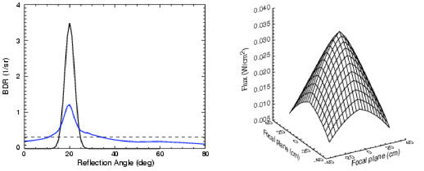
Figure 9: Left: The model incoherent BDR (higher peak) and the measured BDR for primary P3. The model is from equation 2.8.1, with $\sigma=0.4~{}\mu$m, $c=30~{}\mu$m, $\lambda=0.5~{}\mu$m, and $\psi=20^{\circ}$, scaled by 0.09 to match a typical DR. This approximation misses the wings but gets the peak sufficiently well. For the surface upon which the model is based, 13% of the reflected energy is inside a $20^{\circ}$ cone; for P3 this quantity is 11%. The dashed line at $1/\pi$ is for a lossless Lambertian surface. Right: Distribution of power in the focal plane after reflecting off both reflectors.

2.8.3 Microwave Properties of the Aluminum Coating

Aluminum was chosen for the metallic reflector coating because its deposition is well studied and its microwave emissivity is sufficiently low for MAP. For all emissivity calculations, the classical regime obtains: there are no anomalous effects Pippard (1947) and the displacement current can be ignored. Specifically, $\epsilon=4\pi\delta/\lambda=(16\pi\epsilon_{0}f/\sigma)^{1/2}$. Thus the emissivity scales as $f^{1/2}$. At 70 K the emissivity at 100 GHz is about 0.0004 ($\sigma_{300~{}{\rm K}}/\sigma_{70~{}{\rm K}}=0.15$). For two surfaces (primary and secondary) at 70 K, the contribution to the system temperature from the thermal emission is 64 mK at 100 GHz, which is negligible.

Butler (1998) made a precise room temperature measurement of the difference in emissivity between machined stainless steel, copper, aluminum, and vacuum deposited aluminum (VDA) sample with an SiO_x coating. The sample has the same construction as the MAP reflectors except that it is flat. Butler found the differences in emissivity between all materials and the VDA sample to be within 20% of the value computed assuming a conductance of bulk aluminum for the sample. In other words, the VDA coating acts like bulk aluminum at microwave frequencies. Numerous coating samples were checked. No degradation in the microwave properties was observed over a period of a year. No change was seen after thermal cycling to 77 K.

To ensure the similarity of the reflectors, the coating procedure specified that the same prescription be used for symmetric pairs of reflectors. From Figure 8, one sees that with $t>1.2~{}\mu$m, the bulk emissivity should be obtained. To be insensitive to any small variations in the thickness, small defects in the composite surface, or interactions with the composite substrate, a thickness of $t>2.2~{}\mu$m was specified. This is many times the 90 GHz skin depth of $0.11~{}\mu$m at 70 K.

The calculation for Figure 8 is based on the emissivity of a single thin sheet of aluminum at normal incidence. One can be more ambitious and include the XN70 substrate but the results are essentially unchanged: the net emissivity is dominated by the outer most layer of aluminum. The dominant effect in determining the emissivity is the impedance mismatch between the vacuum and the aluminum, for which the index $n_{Al}\approx 2000+i2000$ at 90 GHz.

2.8.4 Spacecraft Charging

Surface charging is a well-known and potentially serious problem for spacecraft. In short, current from the ambient plasma can charge the external surfaces of the S/C to very high potentials ($>10~{}$kV) relative to space or to other spacecraft surfaces. These charged surfaces are subject to abrupt discharge either to a spacecraft surface at a different potential or to space itself. Such high-potential discharges can wreak havoc on the electronics or damage sensitive surfaces. The problem is complicated and empirical. The physical processes include photo ionization, electron and proton current densities, secondary electron densities produced by collisions with the S/C, space charge regions, etc. Jursa (1985).

The surface charging is large when the spacecraft is between 6-10 Earth radii (geosynchronous orbit is 5.6 $R_{E}$) and when there is high geomagnetic activity. Current flow from photoionization by the Sun tends to lower the magnitude of charging from the ambient plasma. Thus, a classic scenario for a discharge event would be entry into (or emergence from) eclipse into sunlight. It is believed to be possible to reach $-25,000~{}$V (relative to infinity), though $-5000~{}$V is more typical. The plasma energies are typically about 10 keV and the currents into the spacecraft are of order 1 nA/cm². The L₂ environment ($\approx 240~{}R_{E}$) is affected by the interaction of the Earth’s magnetic field and the solar wind Evans et al. (2002). As the orientation between the Earth and Sun changes, L₂ moves through different charging environments the most dangerous of which is believed to be the magnetosheath. It is possible that MAP will experience $\leq 25$ keV electrons with a current density of 0.1 nA/cm² from this source.

If the SiO_x is too thick, it insulates the primary. The NASCAP program Jursa (1985) indicates that a $2.5~{}\mu$m layer charges to $\approx-160~{}$V. Tests made on a 150 K sample surface with charged contacts and an electron beam showed that the surface would not abruptly arc with up to 450 V and currents $\approx 10$ nA/cm². The surface instead discharges in a self limiting manner.

3 Performance and Characterization of Optical Design

MAP’s radiometric sensitivity is a result of intrinsically low-noise transistors in a HEMT amplifier that operates over roughly a 20% bandwidth Pospieszalski et al. (2000); Jarosik et al. (2003). The characterization of the optical system takes this bandwidth into consideration. In radio astronomy parlance, MAP is a “continuum” receiver. MAP is characterized primarily in flight through measurements of the CMB dipole, planets, and radio sources. Because of the wide bandwidth, sources with different spectra have different effective frequencies and beam sizes, even within one band.

Two fundamental assumptions about celestial sources are made that allow one to characterize the response as an integral of the response at each frequency. They are: a) signals received at different frequencies are incoherent and b) signals received from different points on a source are incoherent Thompson et al. (1986).

In a perfectly balanced differencing assembly (DA), the output of any one detector switches at 2.5 kHz from being proportional to the power entering side A to the power entering side B. The A$-$B response is synchronously demodulated, integrated for 25.6 ms, and averaged. With the 2.5 kHz phase switch in one position, the power delivered to a diode detector, from one polarization of one feed when viewing a source of surface brightness $S_{\nu}$, is given by

$$W(\alpha,\beta,\gamma)={1\over 2}\int\int\alpha_{l}(\nu)\eta_{R}(\nu)A_{e}(\nu)f(\nu)\,S_{\nu}(\vec{\Omega})\,$$

$$\times B_{n}(\nu,R_{\alpha\beta\gamma}\vec{\Omega})\,d\Omega d\nu,$$ (19)

where $f(\nu)$ is the normalized bandpass of a DA at a reference plane at the OMT/feed interface, and $\alpha_{l}$ accounts for the loss in the microwave components. The feed and antenna losses are included in the radiation efficiency $\eta_{R}$. The normalized beam power pattern $B_{n}(\nu,\vec{\Omega})$, and the effective collecting area of the antenna at normal incidence, $A_{e}(\nu)$, have been expressed separately. Where appropriate in the following, their product is written as $A_{eB}(\nu,\Omega)$. $S_{\nu}(\vec{\Omega})$ is a surface brightness with units of ${\rm W\,m^{-2}sr^{-1}Hz^{-1}}$ and is defined with respect to a fixed coordinate system. The beam is measured in its own coordinates and $R_{\alpha\beta\gamma}$ is the matrix that specifies the beam position and orientation on the sky.

The gain of the optics is measured with a standard gain horn at the GSFC/GEMAC facility. The measurement accuracy is $\pm 0.2$ dBi. The peak gain is measured at 500 frequencies across the band. Full beam maps are made at twelve frequencies per band. The outer two measurements are approximately 10% beyond the nominal passband, two more are at the band edges, and the remaining eight are equally distributed across the band. No phase information is required or used in the analysis.

The loss in the system comes from the optics, $\eta_{R}$, and the radiometer chain, $\alpha_{l}$. In practice, the overall level of both of these is calibrated out and so only their frequency dependence affects the characterization. The dependence of $\alpha_{l}$ is accounted for in the measurement of $f(\nu)$ and so it is dropped in the following. The dependence on $\eta_{R}(\nu)$, which is expected to be small, is found by calculation and so it is retained. For the values in the tables, we take $\eta_{R}=1$ across the passband.

3.1 Response to Broadband Sources

There are a number of possible definitions of the effective area, gain, frequency, and bandwidth. We choose ones that reduce naturally to those for a thermal emitter. To this end, a source is modeled as

$$S_{\nu}(\vec{\Omega})=\sigma(\nu)S(\vec{\Omega}),$$ (20)

where $\sigma(\nu)$ is $\propto\nu^{-0.7}$ for synchrotron emission, $\propto\nu^{-0.1}$ for bremsstrahlung or free-free emission, $\propto\nu^{2}$ for Rayleigh-Jeans emission, $\propto\nu^{3.5}$ for dust emission, and a Planck blackbody at 2.725 K. The total power received is

$$W(\alpha,\beta,\gamma)={1\over 2}\int A_{e}^{bb}(R_{\alpha\beta\gamma}\vec{\Omega})S^{bb}(\vec{\Omega})d\Omega,$$ (21)

where the broadband effective area is defined as

$$A_{e}^{bb}(\Omega)\equiv{\int\eta_{R}(\nu)f(\nu)\sigma(\nu)A_{eB}(\nu,\Omega)d\nu\over\int\eta_{R}(\nu)f(\nu)\sigma(\nu)d\nu}.$$ (22)

and the frequency weighted source function is defined as

$$S^{bb}(\vec{\Omega})\equiv S(\vec{\Omega})\int\eta_{R}(\nu)f(\nu)\sigma(\nu)d\nu~{}~{}~{}{\rm(W/m^{2}\,sr)}.$$ (23)

The effective area is never measured and is only defined through equation 22. If the source is a spatially uniform Rayleigh-Jeans emitter at temperature $T$, then $\sigma(\nu)=2\nu^{2}k_{B}/c^{2}$ and with a flat passband

$$W=(k_{B}\,T/c^{2})\int\int\nu^{2}A_{eB}(\nu,\vec{\Omega})d\Omega d\nu=k_{B}T\Delta\nu.$$ (24)

The broadband gain is defined as

$$g^{bb}(\vec{\Omega})\equiv{4\pi A_{e}^{bb}(\vec{\Omega})\over\int A_{e}^{bb}(\vec{\Omega}^{\prime})d\Omega^{\prime}}={\int\eta_{R}(\nu)f(\nu)\sigma(\nu)g(\nu,\vec{\Omega})/\nu^{2}\,d\nu\over\int\eta_{R}(\nu)f(\nu)\sigma(\nu)/\nu^{2}\,d\nu}$$ (25)

where $g(\nu,\vec{\Omega})$ is the quantity given by computer models of a lossless system. Any measurement includes an error in the calibration, $\pm 0.2$ dBi, and antenna loss $\eta_{R}(\nu)$, though the reflector loss is of marginal importance even in W band. Generally, it is found that the measured forward gain $g_{m}^{bb}$ is $\approx 0.3$ dBi lower than ideal gain, $4\pi/\Omega_{m}^{bb}$, as a result of some loss and slightly more scattering out of the main beam than is accounted for in the models.

The effective frequency of the radiation is given by

$$\nu_{e}\equiv{\int\nu f(\nu)\eta_{R}(\nu)A_{e}(\nu)\sigma(\nu)d\nu\over\int f(\nu)\eta_{R}(\nu)A_{e}(\nu)\sigma(\nu)d\nu}.$$ (26)

Implicit in this definition, and others in which $A_{e}$ explicitly appears, is that the source is smaller than the beam. If a source fills $4\pi~{}$sr, then there would be no dependence on the beam solid angle. This is the reason that the numbers reported here are different from those in Jarosik et al. (2003). The effect is that as one probes higher $l$ the effective center frequency, and therefore the Rayleigh-Jeans to thermodynamic correction, changes.

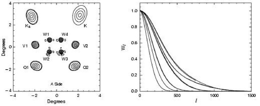
Figure 10: Left: The predicted beam profiles for cooled and distorted optics for a thermal source. If the beams could illuminate the sky, this is the pattern one would see projected on the sky as viewed from the spacecraft. If one looks at the B side focal plane array, as shown in Bennett et al. (2003), the corresponding feeds are left-right reversed. The contours are 0.9, 0.6, 0.3, 0.09, etc. the beam maximum. The small lobes off the W-band beams are the result of the reflector distortions which are greater on the B side than the A side. The lowest contour in W-band is at 0.03. With the measurements combined with the computer code, the beams may be modeled to sub-percent accuracy. The beams in flight will be additionally smeared due to rotation of the satellite. Right: The predicted B-side window functions adjusted for rotational smearing. From left to right on the plot, the windows correspond to K through W “lower” and then the W “upper” beams.

For estimating antenna temperatures and power levels, the effective bandwidth is convenient. It is defined as

$$\Delta\nu_{e}\equiv\biggl{(}12{\int f(\nu)\eta_{R}(\nu)A_{e}(\nu)\sigma(\nu)(\nu-\nu_{e})^{2}d\nu\over\int f(\nu)\eta_{R}(\nu)A_{e}(\nu)\sigma(\nu)d\nu}\biggr{)}^{1/2}$$ (27)

The factor of 12 makes a flat bandpass have a width of $\Delta\nu$. This quantity does not enter into any calculation and is distinct from the noise passband Dicke (1946), $\Delta_{n}\nu$, quoted in Jarosik et al. (2003).

The flux from point-like radio sources is given as $F_{\nu}=\int_{\Omega}S_{\nu}(\Omega)d\Omega$ where $F$ is measured in Janskys ($10^{-26}$ W m^-2Hz^-1). For a narrow frequency band,

$$T_{A}\Delta\nu={1\over 2k_{B}}\int{G_{m}(\nu)c^{2}\over 4\pi\nu^{2}}F_{\nu}d\nu\rightarrow{A_{e}\over 2k_{B}}F_{\nu}\Delta\nu$$ (28)

The usual notation is $T_{A}=\Gamma F_{\nu}$. In the literature, the flux is modeled as $F_{\nu}\propto(\nu/\nu_{e})^{\alpha}$ where $\alpha=2$ for a Rayleigh-Jeans emitter and $\nu_{e}$ is given by equation 26. Since $\Gamma$ depends on the illumination of the primary, it will be similar for all bands. For a “flat spectrum” source, $F_{\nu}$ is independent of frequency ( $\alpha=0$) and has approximately the signature of free-free emission. Such a source has the same approximate antenna temperature in each band.

Implicit in the above is that $B_{n}=1$ at all frequencies. In other words, there is no dependence on the beam. The broad band conversion factor is given by

$$\Gamma^{bb}={(c^{2}/8\pi k_{B}\nu_{e}^{\alpha})\int f(\nu)\eta_{R}(\nu)G_{m}(\nu)\nu^{\alpha-2}d\nu\over\int f(\nu)d\nu}$$ (29)

From the twelve beam measurements the beam characteristics for each source are computed. For the CMB, the predictions of $g^{bb}$ are shown in Figure 10 for what is expected at L₂. Table 8 shows how the effective broad band quantities depend on the source. The actual flight values will be different. The ellipsoidal shape of the low frequency bands results from their large distance from the optimal focal position. The MAP scan strategy has the effect of symmetrizing the beams, mitigating some of the effects of asymmetric beams. The small lobes in the cross pattern on the W and V band beams are a result of the deformations in the mirror from the cool down distortion. Though the distorted beams will complicate the analysis, they are well understood, can be modeled to the sub percent level, and will be measured multiple times in flight.

Table 8: Typical Pre-flight Effective Center Frequencies, Passbands, & Gains for Ideal Beams

Band designation	K	${\rm K_{a}}$	Q	V	Wlow	Wup
Freq range (GHz)	20-25	28-37	38-46	53-69	82-106	82-106
Noise bandwidth, $\Delta_{n}\nu$ (GHz)	5.2	6.9	8.1	10.5	19.0	16.5
%Band	22.6	20.6	19.6	17.2	20.2	17.6
Synchrotron: $S_{\nu}\propto\nu^{-0.7}$
$\nu_{e}$ (GHz)	22.4	32.6	40.5	60.5	94.9	93.0
$\Delta\nu_{e}$ (GHz)	5.7	7.2	8.5	13.9	22.3	17.7
Free-free: $S_{\nu}\propto\nu^{-0.1}$
$\nu_{e}$ (GHz)	22.5	32.7	40.6	60.7	93.0	93.1
$\Delta\nu_{e}$ (GHz)	5.7	7.2	8.5	14.0	22.5	17.8
$\Gamma^{bb}$ ($\mu$K/Jy)	250	230	240	240	240	270
Rayleigh-Jeans: $S_{\nu}\propto\nu^{2}$
$\nu_{e}$ (GHz)	22.8	33.0	41.0	61.3	93.7	93.9
$\Delta\nu_{e}$ (GHz)	5.5	7.0	8.3	14.0	23.0	18.0
$\Omega^{bb}_{m}$ (deg2)	0.77	0.44	0.26	0.12	0.052	0.044
$A^{bb}_{e}$ (m2)	0.72	0.60	0.67	0.66	0.61	0.76
$g^{bb}$ (dBi)	47.1	49.8	51.7	55.5	58.6	59.3
Dust: $S_{\nu}\propto\nu^{3.5}$
$\nu_{e}$ (GHz)	23.0	33.1	41.1	61.5	94.2	94.5
$\Delta\nu_{e}$ (GHz)	5.2	6.9	8.1	14.0	19.0	18.1

3.2 Window Functions

The statistical characteristics of the CMB are most frequently expressed as an angular spectrum of the form $l(l+1)C_{l}/2\pi$ Bond (1996) where $C_{l}$ is the angular power spectrum of the temperature:

$$T(\theta,\phi)=\sum_{l,m}a_{lm}Y_{lm}(\theta,\phi),~{}~{}~{}C_{l}=<|a_{lm}|^{2}>.$$ (30)

The spherical harmonic expansion is written so that $T(\theta,\phi)$ is real. The beam acts as a low pass filter on the angular variations in $T(\theta,\phi)$, smoothing the sky over a characteristic gaussian width of $\sigma_{b}=\theta_{fwhm}/\sqrt{8\ln(2)}$. The variance of the time stream one would measure at the output of a noiseless detector as the beam scans the sky is

$$\approx\sum_{l}{(2l+1)C_{l}\over 4\pi}W_{l}$$ (31)

where $W_{l}$ is the window function which encodes the beam smoothing. In practice, one works with maps in which each pixel has been traversed in multiple directions by an asymmetric beam. Then, one determines the variance of the ensemble of pixels as a function of $l$ and $\Delta l$. The full window function for a separation of the beam centroids of $\theta_{12}$ is

$$W_{l}^{\gamma_{1}\gamma_{2}}(\theta_{12})=\biggl{(}{1\over\Omega_{A}^{2}}\biggr{)}\int\int P_{l}(\cos(\theta_{12}^{\prime}))B_{n}(R_{\gamma_{1}}\vec{\Omega}_{1},\vec{\Omega}_{1}^{\prime})\times$$

$$B_{n}(R_{\gamma_{2}}\vec{\Omega}_{2},\vec{\Omega}_{2}^{\prime})d\Omega_{1}^{\prime}d\Omega_{2}^{\prime}\hskip 72.26999pt$$ (32)

where $R_{\gamma}$ gives the orientation of the beams. The full expression with orientable asymmetric beams has been used by Cheng et al. (1994), Netterfield et al. (1997), Wu et al. (2000), and Souradeep & Ratra (2001). For the zero lag window with symmetric beams, $W_{l}=B_{l}^{2}/\Omega_{A}^{2}$ where $B_{l}=2\pi\int B_{n}(\theta)P_{l}(\cos\theta)d(\cos\theta)$ and $P_{l}$ are the Legendre polynomials. If the beams are Gaussian, $W_{l}=\exp(-(l+1/2)^{2}\sigma_{b}^{2})$.

On the right side of Figure 10 are shown the window functions for the B-side beams after they have been circularly symmetrized. As the derived angular spectrum is directly multiplied by $W_{l}$ Oh et al. (1999), some care must be taken in determining the window. The flight values will be different from those shown and will be quantified with both models and in-flight beam maps.

3.3 Practical Issues

MAP makes differential measurements and thus measures the difference in power from radiation received from opposite sides of the spacecraft. The relevant quantity from which the maps are derived is

$$W_{D}^{\gamma_{1}\gamma_{2}}(R_{\gamma_{1}}\vec{\Omega}_{1}-R_{\gamma_{2}}\vec{\Omega}_{2})={1\over 2}\int\int\bigg{\{}\alpha_{A}\eta_{A}A_{e,A}(\nu)f_{A}(\nu)$$

$$\times S_{\nu}(\vec{\Omega}_{1}-\vec{\Omega})\,B_{n,A}(\nu,R_{\gamma_{1}}\vec{\Omega}_{1},\vec{\Omega}))-\hskip 57.81621pt$$ (33)

$$\alpha_{B}\eta_{B}A_{e,B}(\nu)f_{B}(\nu)\,S_{\nu}(\vec{\Omega}_{2}-\vec{\Omega})\,B_{n,B}(\nu,R_{\gamma_{2}}\vec{\Omega}_{2},\vec{\Omega})\,\bigg{\}}d\vec{\Omega}d\nu.$$

for two different directions $\vec{\Omega}_{1}$ and $\vec{\Omega}_{2}$ for the ’A’ and ’B’ sides respectively. Even if $\vec{\Omega}_{1}$ and $\vec{\Omega}_{2}$ are switched (the A-side points to where the B-side was), $f_{A}=f_{B}$, $\alpha_{A}=\alpha_{B}$ (the phase switch is in the same position and the hybrids, waveguides, and OMT are matched), and $A_{e,A}=A_{e,B}$, $W_{D}$ is not zero. This is because $B_{n,A}$ and $B_{n,B}$ are not the same. The differential pairs are back-to-back and far from the ideal focus. In reality, $f_{A}\neq f_{B}$, $\alpha_{A}\neq\alpha_{B}$, and $A_{e,A}\neq A_{e,B}$, though to first order the small differences will be calibrated out. In the end, though, the different beams will have to be taken care of in the analysis. Because Jupiter is so bright, each of the forty beam profiles will be independently mapped.

4 Systematic Effects

Systematic effects associated with the optics such as beam size, sidelobe levels, and the effective frequency directly affect the scientific interpretation of the data. In this section, systematic effects associated with the stability and integrity of the optical system are discussed.

The largest systematic effects are associated with infrared and microwave emission from the Sun, Earth, and Moon whose properties, as viewed from L₂, are summarized in Table 9.

Table 9: Parameters for Sun, Earth, and Moon, from L₂

	Sun	Earth	Moon
Temperature, Ts (K)	6000	300	250
Distance from L2, $d_{s}$ (m)	$1.5\times 10^{11}$	$1.5\times 10^{9}$	$1.5\times 10^{9}$
Radius, $r_{s}$ (m)	$7\times 10^{8}$	$6.4\times 10^{6}$	$1.7\times 10^{6}$
$I_{inc}^{ir}$ Flux at L2 (W/m2)	1600	$8.5\times 10^{-3}$	$2.8\times 10^{-4}$
Solid Angle from L2 (sr)	$6\times 10^{-5}$	$6\times 10^{-5}$	$5.3\times 10^{-6}$
$I_{inc}^{mw}/A$ in $\Delta\nu=24~{}$GHz (W/m2)	$2.4\times 10^{-8}$	$1.0\times 10^{-9}$	$1.1\times 10^{-10}$
$\rm T_{eff}$ (mK)	130	5.5	0.6

4.1 Thermal Variation of Optics

The S/C is oriented so that the angle between the Sun and the symmetry axis is constant during the spin and precession. Thus, the thermal loading remains constant for long periods. The radiators are designed so that they are $2\fdg 2$ degrees inside the Sun’s shadow at all times. The reflectors too are $>6\hbox{${}^{\circ}$}$ inside the Sun’s shadow. Infrared emission from the Earth and the Moon, however, can directly illuminate the primary as can be seen in Figure 1. In the following, conservative order-of-magnitude estimates are made of the anticipated radiometric signal due to heating of the primary.

The primary is a complicated composite structure with multiple thermal time constants and can only be treated roughly in isolation. An input of thermal power, $\Gamma^{t}$, heats up the mirror. The energy in turn is both immediately reradiated and flows to other parts of the S/C where it is eventually reradiated. The energy flow for both mechanisms is modeled as

$$C_{M}{dT\over dt}+g^{th}(T-T_{0})=\Gamma^{t}$$ (34)

where the heat capacity is $C_{M}$ and $g^{th}$ is the thermal conductance. The solution to equation 34 with a step function change in incident power is:

$$T=T_{0}+\Gamma^{t}(1-e^{-t/\tau})/g^{th}$$ (35)

where $\tau=C_{M}/g^{th}$.

The dominant conductive path is through the $0.0254$ cm thick composite skin of the reflector. The thermal conductivity of the XN70 is $\kappa_{s}=0.19$ W cm^-1K^-1 at 70 K, more than twice that of stainless steel. The composite’s density is $\rho_{s}=1.8~{}{\rm gm\,cm^{-3}}$ and the specific heat capacity is $c_{s}=200~{}{\rm J\,kg^{-1}\,K^{-1}}$. The characteristic time for a heat pulse to propagate $l_{h}=20$ cm is $\tau_{cond}=l_{h}^{2}\rho_{s}c_{s}/\pi^{2}\kappa_{s}^{2}\approx 80~{}$s, though the full solution is a series expansion in time constants and depends on geometry Hildebrand (1969).

The emitted radiation, for small temperature variations, is linearized so that $\delta I_{rad}=4\epsilon_{ir}\sigma T_{0}^{3}\delta T$. The effective radiating area is the face of the primary with $A_{rad}=1.76~{}$m² for which the emissivity is taken as $\epsilon_{ir}=0.1$ at $\lambda=30~{}\mu$m. (At $\lambda=10~{}\mu$m and 300 K, $\epsilon_{ir}=0.5$.) The conductance is given by $g^{th}_{rad}=4\epsilon_{ir}\sigma T_{0}^{3}A_{rad}=0.015~{}$W/K at 70 K. The heat capacity is difficult to estimate and depends on the coupling between the reflector surface and its backing structure. If the whole 5 kg reflector heats up, then $c_{s}\approx 250~{}{\rm J\,kg^{-1}\,K^{-1}}$, the heat capacity of a typical composite, and $C_{M}\approx 1000~{}$J K^-1. If just the thin surface heats up, then $C_{M}\approx 160~{}$J K^-1, leading to the range $3~{}{\rm h}<\tau_{rad}<20~{}{\rm h}$. Because $\tau_{cond}>>\tau_{rad}$, to a good approximation the primary first thermalizes and then radiates.

To estimate $\Gamma^{t}=\epsilon_{ir}I_{inc}^{ir}A_{il}$ it is assumed that the Earth (Moon) illuminates $A_{il}\approx{\rm 0.15~{}m^{2}}$ ( $A_{il}\approx{\rm 1~{}m^{2}}$) with an absorptivity of $\epsilon_{ir}\approx 0.1$. For the Earth, $\Gamma^{t}_{E}=1.3\times 10^{-4}~{}$W and for the Moon, $\Gamma^{t}_{M}=3\times 10^{-5}~{}$W. The temperature increase for a long exposure ($>\tau_{rad}$) is $\Gamma^{t}/g^{th}_{rad}$. For the Earth, this is $\Delta T_{phys}\approx 9~{}$mK and for the Moon it is $\Delta T_{phys}\approx 2~{}$mK. The precise illumination depends on the orbit, spacecraft orientation, and blockage of the radiation by the secondary as shown in Figure 1 and so these estimates should be considered conservative upper limits.

The rotation period of the satellite is 132 s. The reflectors have a good view of the Earth and Moon over about $45\hbox{${}^{\circ}$}$ range, or for about $\tau_{obs}=15~{}$s. In the limit that the heat is first conducted away from the heated area and later reradiated, equation 35 gives a temperature change of $\Delta T_{phys}=1.5~{}$mK for the Earth and $\Delta T_{phys}=0.35~{}$mK for the Moon. The radiometric signal is proportional to the thermal variation multiplied by the microwave emissivity integrated over the beam response. In W-band, the optical response near the top of the primary, where the Earth illuminates it, is $\approx-5~{}$dB of the peak and so the expected radiometric signal is $\approx 0.5~{}\mu$K. The Moon illuminates the central part of the primary and so the expected radiometric signal is $\approx 0.4~{}\mu$K. The primaries, secondaries, and radiators are instrumented with platinum resistive thermometers (PRTs) to detect a 0.5 mK change in one rotation. These measurements and a detailed thermal model will be used to model the on orbit performance.

The estimates above assume the same emissivity on both sides but variable thermal loading. If the microwave emissivity of the two reflector systems is different and the temperatures of both move up and down identically, then a signal will result. If the temperature of the reflectors change together by 10 mK, which is conservative but not impossible, then the differential signal changes by $1~{}\mu$K if $\delta\epsilon/\epsilon=0.2$.

Finally, because the current distributions from each feed overlap on the primary, as shown in Figure 2, temperature and emissivity gradients will have a common-mode effect on all channels. This will aid in characterizing any variations in the optics.

4.1.1 Emission From a “Dirty” Surface.

The reflector surfaces are specified to be “visibly clean.” In contamination engineering, a visibly clean surface has $500<l_{c}<700$, where $l_{c}$ is the “cleanliness level.” For example, a surface with one $3~{}\mu$m by $30~{}\mu$m needle per square millimeter (0.01% obscuration) results in $l_{c}=400$. If the particles are spherical with the same fractional obscuration, $l_{c}=250$. These surfaces would pass as visibly clean. On the other hand, a surface covered with $20~{}\mu$m by $100~{}\mu$m needles with a 2% surface obscuration results in $l_{c}>1000$ and is clearly not visibly clean. This corresponds to 1 g of graphite spread over the surface. Generally, the unaided eye can detect $50~{}\mu$m particles.

During the integration and prelaunch phase, the optical surfaces are constantly purged and kept clean. However, the fairing separation soon after launch can produce a cloud of debris. Even though the MAP payload fairing was specially cleaned and inspected to minimize the possibility of contamination, it was estimated that there could be 1 g of contaminating material and one ${\rm 1\times 5~{}cm^{2}}$ piece of fairing tape within the area of one reflector. The energetics and geometry of the separation strongly disfavor much, if any, of this material sticking to the primary. Of the possible contaminants shown in Table 10, graphite is the most pernicious.

Surface dust or debris increases the microwave emissivity possibly resulting in a radiometric signal. The magnitude of the signal depends on the material’s coupling to the surface. For a piece of ${\rm 1\times 5~{}cm}^{2}$ $0.05~{}$cm thick Mylar tape, the most pessimistic case occurs when the contaminant is attached at the center of the primary in a way such that its response to temperature variations is instantaneous and its emissivity is unity in the infrared and $\epsilon_{eff}=0.03$ at 90 GHz as shown in Table 10. The maximum radiometric temperature will be

$$\Delta T_{rad}=\epsilon_{eff}\Delta T_{object}{A_{object}\over A_{il}}\approx 0.15~{}\mu{\rm K}.$$ (36)

where $A_{il}\sim 10^{4}~{}{\rm cm}^{2}$ is the illumination area of the beam, and $T_{object}\sim 10~{}$mK.

Though there will be some graphite in the mix of debris, there is far less than 1 gm. If, though, 1 gm of the 20 $\mu$m by 100 $\mu$m needles discussed above is distributed over the surface there are roughly 10 particles per mm². Needles this close to the reflector will follow the surface temperature. Since they are much smaller than a wavelength and in the node of the electric field their effective emissivity is small. The power in the standing wave as a function of distance $z$ from the surface is proportional to $\sin(4\pi z/\lambda)$. A $20~{}\mu$m diameter grain at 90 GHz on the surface sees a reduction in power of $\approx 10^{-3}$ after accounting for the radiation reflected to the scatterer from the mirror. Thus we assume $\epsilon_{eff}\approx 0.001$. The emission temperature is then $\epsilon_{eff}T_{phys}A_{objects}/A_{il}\approx 0.02~{}\mu$K.

We can never be certain how much contamination ends up on the surface. The effective emission temperatures for large pieces of material and for graphite grains are conservative upper limits. They are meant to show MAP’s immunity to contamination.

4.2 Thermal Variation of the Radiators

Sun light diffracts over the edge of the sun shield and illuminates the radiator at a very low level. As the S/C spins this term is modulated, leading to a temperature variation of the radiator and in turn the HEMT amplifiers. Using GTD around the edge of the solar shield, a conservative estimate shows that no more than 0.1 W could be absorbed by the radiator. The heat capacity of a radiator panel is $C_{r}=2500$ J K^-1 and so the temperature variation is $\approx 0.1~{}{\rm W}C_{r}^{-1}\tau_{obs}=50~{}\mu$K for $\tau_{obs}=1~{}$s. With an emissivity of $<$1%, the maximum radiometric signal is $1~{}\mu$K for perfect radiometric coupling. Because the heat is injected at the outer edge of the radiator, far from the optics, and it is partially reradiated, the resulting radiometric signal is $<<1~{}\mu$K.

Table 10: Possible contaminants at 90 GHz

Potential contaminant	$\epsilon$	Re($\epsilon$ )	Im($\epsilon$ )	$\alpha$ (cm-1)	Source
Graphite	$\epsilon=700+i(4.8\times 10^{-3}\nu^{1.13}+1.5\times 10^{7}/\nu)$	700	170000	…	Draine & Lee (1984)
Eccosorb CR110	$\epsilon\approx 3.53+i0.48\,\nu^{0.1}$	3.53	…	2.0	Halpern (1986)
Ice	$\epsilon=3.155+i2.8\times 10^{-4}\nu$	3.155	0.026	…	Koh (1997)
Mylar	$\epsilon\approx 2.82+i(0.15+1.7\times 10^{-4}\nu)$	2.8	0.17	0.52	Page et al. (1994)
Silicates	$\epsilon=11.8+i1.1\times 10^{-3}\nu$	11.8	0.1	…	Draine & Lee (1984)
SiO2	$\epsilon\approx 3.8+i9\times 10^{-4}\nu^{1.51}$	3.8	0.8	0.003	Mon & Sievers (1975)

4.3 Scattering of Light from the Sun, Earth, & Moon by Contamination on Primary

Microwave power from the Moon and Earth can scatter off debris on the reflector and potentially produce a glint as the S/C rotates. The form of the contamination is not known and so several possibilities are considered. The differential cross section Van de Hulst (1981); Landau & Lifshitz (1984) for the scattering of unpolarized incident light from an isotropic medium is

$${d\sigma\over d\Omega}=\biggl{(}{2\pi\nu\over c}\biggr{)}^{4}|\alpha_{p}|^{2}{(1+\cos^{2}\theta_{s})\over 2},$$ (37)

where $\alpha_{p}$ is the polarizability of the material, $V$ is the volume, and $\theta_{s}$ is scattering angle. In the following, the angular term is taken as 3/4 and the scattering from each grain is treated as isotropic.

The polarizability of a needle and a sphere respectively are given by

$$\alpha_{p}^{needle}={1\over 4\pi}(\epsilon-1)V~{}~{}\&~{}~{}\alpha_{p}^{sphere}={3\over 4\pi}\biggr{(}{\epsilon-1\over\epsilon+2}\biggl{)}V,$$ (38)

where $\epsilon$ is the dielectric constant and $V$ is the grain volume. The most efficient scattering shape per unit volume is a needle.

If light with flux (power/area) strikes the scatterer, the intensity at scattering angle $\theta_{s}$ and distance $r$ is

$$I_{sca}(\theta_{s})={d\sigma\over d\Omega}I_{inc}^{mw}/r^{2}$$ (39)

For a random set of incoherent scatterers with surface density $\sigma_{N}$, the scattered power adds. Thus, the total scattered light is just $\sigma_{N}A$ times the above, where $A$ is the area covered by the scatterers. This surface element subtends a solid angle of $A\cos\theta_{o}/r^{2}$. Thus, the resulting surface brightness is

$$B_{sca}(\theta_{s})=\sigma_{N}{d\sigma\over d\Omega}I_{inc}^{mw}/(\cos\theta_{o}\Delta\nu)~{}~{}~{}~{}~{}{\rm W\,m^{-2}\,sr^{-1}\,Hz^{-1}}.$$ (40)

The $\cos\theta_{o}$ in the denominator accounts for isotropic scattering; the scattering is not Lambertian.

The equivalent parabola concept (Table 1) is used to compute the measured signal. The scattered light from the top of the primary is modeled as directly entering the feed. The Moon illuminates $\approx 0.2~{}$sr of the primary at an angle from the feed of $\theta_{o}\approx 20^{\circ}$ and gain of 20 (13 dBi) as indicated in Figure 1. The Earth, though hotter, illuminates less and is subdominant. Because of the large uncertainty in the type of contaminant, a full integration of the telescope response is not necessary. The effective antenna temperature is given by:

$$T_{A}={1\over 4\pi}\int{B_{sca}(\theta)\lambda^{2}\over 2k_{B}}g(\theta_{o})d\Omega\hskip 72.26999pt$$ (41)

$$=(3/16)\eta_{surf}\sigma_{N}\biggl{(}{2\pi\nu\over c}\biggr{)}^{4}|\alpha_{p}|^{2}T_{s}(r_{s}/d_{s})^{2}g(\theta_{o})\Delta\Omega.$$

where $r_{s}$, $d_{s}$, and $T_{s}$ are given in Table 9. The efficiency $\eta_{surf}$ encodes the fact that the scatterers on a metal surface are at the node of the electric field. For lunar emission at 90 GHz, equation 41 becomes $T_{A}=7\times 10^{9}\eta_{surf}\sigma_{N}|\alpha_{p}|^{2}$ in MKS units.

For the $20~{}\mu$m by $100~{}\mu$m needles at 90 GHz discussed above, $\eta_{surf}\approx 10^{-3}$, $\sigma_{N}={\rm 10^{7}m^{-2}}$, $|\alpha_{p}|^{2}/V^{2}\approx 2\times 10^{9}$, and $V=3\times 10^{-14}~{}{\rm m^{3}}$. The result is that $T_{A}=120~{}\mu$K. If the mass of graphite is held fixed but the shape of the grain is more spherical, $T_{A}$ is reduced to sub-$\mu$K levels. Baring the pathological case of large needles, emission from scattering off contaminants is negligible.

4.4 Nonuniform Coating of Primary

It is possible that the primary may be coated with a thin layer of water or hydrazine (fuel for the thrusters) which then freezes. Neither of these absorbs microwave radiation but if they irregularly coat the surface the variation in the thickness of material leads to a variation in the phase of the wavefront in turn leading to a distortion of the beam. The phase delay for a thickness $d$ is $\delta\phi=2dn/\lambda$. For example, if 1 g of water freezes out over half the surface, $\delta\phi\approx 1.4\times 10^{-3}$. This is negligible, more than two orders of magnitude smaller than the surface rms specification discussed in section 2.6

4.5 Micrometeoroids

Micrometeoroids pelt the optics, thereby increasing their microwave emissivity. The particle distribution Anderson (1998); Best (1998) shown in Figure 11 is typical for Earth spacecraft, and believed to be representative of L₂. The relative velocity to the S/C is $19$ km/sec and they may hit at any angle. At the heavy end of the distribution, the particles have an energy of $50$ J. Each penetration is modeled as a circular hole of diameter the micrometeoroid multiplied by a factor. Holes in the sun shield transmit a negligible amount of solar energy; holes in the reflectors might act as blackbodies at 70 K, the temperature of the reflectors.

The micrometeoroids have a size distribution between 15$~{}\mu$m and 700$~{}\mu$m and a mass between 0.004 $\mu$g and 400 $\mu$g. They are mostly olivines and silicates. The specific density for particles under 1 $\mu$g is $2$ g/cm³; for masses between 1 $\mu$g and $0.01$ g, it is $1$ g/cm³; and it is $0.5$ g/cm³ for more massive meteoroids. In round figures, there is roughly $1$ hit/m² per year of a $100~{}\mu$m diameter particle and $100$ hits/m² of $10~{}\mu$m diameter particles.

To compute the flux that scrubs the reflectors, the values in Figure 11 are scaled to one month and a surface of $1.8$ m², corresponding to one primary reflector. The holes (places where the Al is removed) are modeled as circular apertures that transmit 90 GHz. For a 300 $\mu$m radius particle, $ka=0.57$ ($a$ is the radius) thus some care must be taken in computing the transmission coefficient. Landau’s expression Jackson (1999) is used even though it is imprecise (though sufficient) near $ka\sim 1$. The power transmission coefficient is

$$\tau_{trans}(ka)=1-\frac{1}{2ka}\int_{0}^{2ka}J_{0}(t)\,dt\approx\frac{{(ka)}^{2}}{3}\quad\mbox{for}\quad ka\ll 1$$ (42)

A perfect mirror, with holes of radii $a_{i}$, $i\in\{1,n\}$, has an effective temperature given by:

$$T_{A}=\frac{\left({\epsilon}_{Al}\left(A_{refl}-\sum_{i}\pi a_{i}^{2}\right)+\sum_{i}\tau_{trans}(a_{i})\pi a_{i}^{2}\right)}{A_{refl}}T_{refl}$$ (43)

where $\tau_{trans}$ is the transmission coefficient of a hole, $\epsilon$ is the emissivity of the coated surface, $T_{refl}$ is the reflector temperature and $A_{refl}$ is its area. We conservatively model the holes as perfect, though small, emitters. This model is valid in the limit of $\sum_{i}\pi a_{i}^{2}<<A_{refl}$ and $\tau_{trans}>\epsilon_{Al}$. For each successive hit,

$$\Delta T_{A}=\frac{\left(-{\epsilon}_{Al}+\tau_{trans}(a_{i})\right)\pi a_{i}^{2}}{A_{refl}}\,T_{refl}$$ (44)

At 94 GHz, $\tau_{trans}\approx\epsilon_{Al}$ for particles with $a<20~{}\mu$m and the simple model breaks down. However, these particles contribute negligibly to the overall emissivity. The primaries and the particle flux on them are assumed to be independent. For each mass bin of index $i$ and each month, the number $n_{i}$ of collisions is randomly chosen for each reflector according to the Poisson distribution. The change in $T_{A}$ for one reflector is given by $n_{i}\times\Delta T_{A}(a_{i})$, where $a_{i}$ is the radius of the particles belonging to the particular mass bin. After adding the individual contributions of all of the bins and taking the difference between reflectors, the result is recorded and the process starts again with a new month.

To assess the net differential signal produced by the collisions, one simulates many MAP missions as shown in Figure 11. The standard deviation of the data is $0.25~{}\mu$K. From the cumulative probability distribution one finds that with 95% probability, the difference in temperatures will be smaller than $0.5~{}\mu$K. Most evidence suggests the holes will be bigger than the particle size. To bound the problem, consider $r_{hole}=5a$. As $\Delta T_{A}\propto\sim~{}a^{4}$ in the $ka<<1$ limit, one expects a distribution 625 times wider. However, for the largest particles, $ka\approx 3$, and the small size approximation in equation 42 is not valid. The net effect is that the 95% upper limit on an offset is $140~{}\mu$K.

This offset is virtually undetectable. If MAP were not differential, the net signal from micrometeoroids would not be much different. This is because the damage to the reflector is dominated by relatively few encounters with 100 $\mu$m size particles. With two large reflectors, the cross section doubles and is not compensated by the differential measurement.

In the right hand side of Figure 11 is plotted the average number of collisions per month for the heaviest mass bins. These collisions produce large holes but are rare. Most important, the contribution to the total hole area from the largest particles is not increasing as one moves to yet larger particles, indicating that if the distribution is accurate, $140~{}\mu$K is a reasonable bound on the change in offset. This effect would most likely be masked by other radiometer effects and would, in any case, be strongly suppressed by the mapmaking algorithm and scan strategy.

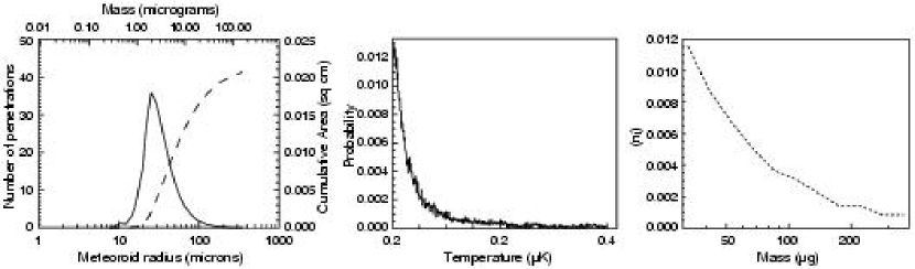
Figure 11: Left:The solid line shows the distribution of the number of penetrations per each of 50 meteoroid radius bins for 15.8 m² area exposed (e.g., the Sun shield) for 27 months (the nominal mission lifetime)Anderson (1998). One assumes that each hit results in a penetration. The dashed line is the cumulative area of the penetrations. Note that most of the net area comes from just a few particles. The radius as a function of mass is computed for a density of $2$ g/cm³ and a spherical shape.Center The normalized probability distribution for 35,000 realizations of $\Delta T$ at the end of 27 months for two mirrors with $r_{hole}=a$. As a consequence of the differential measurement, the mean value is zero. Right: The number of collisions per year for 1.8 m² for each mass bin (dot). The probability of a hit by a particle of diameter larger than 200 $\mu$m hits is 0.2/m² per year, or 0.7 per primary per 27 months.

5 Conclusions

We have designed a differential optical system for performing precise and accurate measurements of the anisotropy in the cosmic microwave background with an angular resolution of $<0\fdg 23$. All major components of the system have been measured and modeled in detail. Such a characterization is required in order to give us confidence in the scientific conclusions we derive from MAP. In addition, we have presented estimates of a number of systematic effects and have shown that in all cases their radiometric contribution to the celestial signal is negligible.

6 Acknowledgements

The development of the MAP optics started in 1993 and has involved many people in addition to the authors. At Princeton, N. Butler, W. Jones, and S. Bradley wrote senior theses on various aspects of the development; C. Bontas worked on the calculations for the micrometeroid and surface deformations; A. Marino, D. Wesley, C. Steinhardt, C. McLeavey, C. Dumont, M. Desai, M. Kesden, A. Furman, O. Motrunich, R. Dorwart, E. Guerra, & C. Coldwell worked on modeling and testing various components; C. Sule, and G. Atkinson worked on building optical components; and S. Dawson, A. Qualls, and K. Warren kept the Princeton effort running smoothly. At UBC, M. Jackson measured the fine scale surface deformations and C. Padwick measured the cryogenic properties of thin aluminum coatings. J. Heaney of Swales along with S. Dummer and R. Garriott of SOC helped define and worked especially hard to produce a surface that met the specifications. D. Neverman at PCI led the team that built the TRS. S. Best and J. Anderson provided the micrometeoroid test data and initial meteoroid flux calculations, respectively. The NASA/GSFC team, led by L. Citrin, the project manager, worked long hours to make the MAP optics a reality. C. Trout-Marx independently verified the design with Code V; S. Seufert and K. Hersey ran the beam mapping effort and K. Hersey verified and ran the beam prediction code at GSFC; T. VanSant led the materials analysis team, supported by a large group including B. Munoz, C. He, L. Wang, and C. Powers; the reflector and blanket surface composition characterization was additionally supported by L. Bartusek, L. Kauder, R. Gorman, and W. Peters; S. Glazer led the thermal predictions group, with key support from D. Neuberger; P. Mule led the STOP verification effort (building on the work of J. McGuire); L. Lloyd and P. Trahan did the PRT harness fabrication and installation; A. Herera, H. Sampler, D. Osgood, C. Aviado, M. Hill, D. Schuster, T. Adams, and M. Holliday made sure that the optics were aligned and blanketed correctly; W. Chen, S. Ngo, and J. Stewart led the mechanical design team at GSFC, with key support from B. Rodini, J. Parker, M. Schoolman, and T. Driscoll; E. Packard led the facility support activities; M. Jones ensured quality assurance; and A. Crane, with support from A. Herrera, N. Dahya, R. Hackley, and M. Lenz, led the TRS I & T effort. The GTD calculations, especially equation 12, were done with J. Mather when he was part of the team (though any errors here are independent of his work). Comments at early design reviews by D. Fixsen, P. Timbie, and P. Napier and the input from a review led by J. Mangus were especially helpful. We also thank B. Griswold of NASA/GSFC for his work on the figures. The modeling of the optics was done with assistance and code from YRS Associates: Y. Rahmat-Samii, W. Imbriale, and V. Galindo. Finally, we thank an anonymous reviewer whose comments improved the paper. This research was supported by the MAP Project under the NASA Office of Space Science and Princeton University. More information about MAP may be found at http://map.gsfc.nasa.gov.

References

- Anderson (1998) Anderson, J. MAP Memorandum to Cliff Jackson, 12 Jan 1998 from NASA/Marshall Space Flight Center.
- Ashcroft & Mermin (1976) Ashcroft, N. W. & Mermin, N. D. 1976, “Solid State Physics,” Holt, Rinehart, and Winston, Philadelphia, PA
- Baker et al. (1999) Baker, J. C et al. 1999, MNRAS, 308, 1173 (astro-ph/9904415)
- Barnes et al. (2002) Barnes, C. et al. 2002, Ap.J.Supp., 143, 567
- Beckmann & Spizzichino (1963) Beckmann, P. & Spizzichino, A. 1963, “The Scattering of Electromagnetic Waves from Rough Surfaces,” Pergamon Press, Macmillan Co. NY
- Bennett et al. (2003) Bennett, C. et al. 2003, ApJ, 583.
- Bennett & Porteus (1961) Bennett, H. E. & Porteus, J. O. 1961, J. Opt. Soc Am. Vol 51, No 2, pp 123
- Benot et al. (2002) Benot, A. et al. 2002, Submitted to A&A, astro-ph/0210305
- Best (1998) Best, S. provided the particle distribution. Auburn University Space Power Institute, Auburn University, Alabama, 36848-5320, private communication.
- Bond (1996) Bond, J., R. 1996, in Cosmology and Large Scale Structure, Les Houches Session LX, ed. R. Schaeffer et al. (Elsevier), 496
- Born & Wolf (1980) Born, M. & Wolfe, E 1980, “Principles of Optics,” 6th ed. Pergamon Press
- Brown & Prata (1995) Brown, K, and Prata, A. 1995, IEEE Trans. Ant. Prop., Vol 42, No. 8, pp 1145-1153
- Butler (1998) Butler, N. 1998, “Emissivity Measurements of MAP Satellite Optics,” Sr. Thesis at Princeton University
- Cheng (1994) Cheng, E. S. et al. Ap.J. 422, L37, 1994 1993, “Emissivity Measurements of MAP Satellite Optics,” Sr. Thesis at Princeton University
- Clarricoats & Olver (1984) Clarricoats, P. J. B., & Olver, A. D. 1984, “Corrugated Horns for Microwave Antennas,” (London: Peter Peregrinus)
- Coble et al. (1999) Coble, K., et al. 1999, ApJ, 519, L5-L8
- Crill et al. (2002) Crill, B. P., et al. 2002, Submitted to Ap.J., astro-ph/0206254
- Davies (1954) Davies, H. 1954, Proc IEE, Pt IV, Vol 101, pp 209-214
- de Bernardis et al. (1994) de Bernardis, P. et al. 1994, ApJ 422, L33-L36
- Devlin et al. (1998) Devlin, M. et al. 1998, ApJ Letters 509:L69
- Dicke (1946) Dicke, R. H. 1946, Rev. Sci, Instr., 17, 268
- Dicke (1968) Dicke, R. H. 1968, “The Theoretical Significance of Experimental Relativity,” Gordon and Breach, New York
- Dragone (1986) Dragone, C. 1986, IEEE Trans. Ant. Prop., Vol AP-34, No. 5, pp 689-701
- Dragone (1988) Dragone, C. 1988, IEEE Trans. Ant. Prop., Vol 36, No. 2, pp 209-215
- Draine & Lee (1984) Draine & Lee 1984, Ap. J. 285, 89-108
- Evans et al. (2002) Evans, S. W. 2002, “Natural Environment Near The Sun/Earth-Moon L2 Libration Point” Prepared for the Next Generation Space Telescope program by the Marshall Space Flight Center. Available through http://www.ngst.nasa.gov/public/unconfigureqd/doc_0761/rev_01
- Galindo-Isreal et al. (1992) Galndo-Isreal, V., Veruttipong, W., Norrod, R., & Imbriale, W. 1992, IEEE Trans. Ant. Prop. Vol 40, No 4, pg 422
- Ganga et al. (1993) Ganga, K., Page, L., Cheng, E. S., & Meyer, S. 1993, ApJ, 410, L57-L60
- Garg et al. (1975) Garg, R., Gupta, K.C., Sharan, R. 1975, Int. J. Electronics, 39, No. 5, pp. 525-527
- Gundersen et al. (1995) Gundersen, J. O., et al. 1995, ApJ, 443, L57
- Halpern (1986) Halpern, M. 1986, Ap. Opt. 26, 4
- Hancock et al. (1997) Hancock, S., et al. 1997, MNRAS 289, 505
- Hanany & Marrone (2002) Hanany, S., and Marrone, D. 2002, Submitted to Applied Optics, astro-ph/02066211.
- Harrison et al. (2000) Harrison, D. L., et al. 2000, MNRAS 316, L24-L28
- Hass et al. (1969) Hass, G., Ramsey, J. B. Heaney, J.B., Triolo, J.J. 1969, “Reflectance, Solar Absorptivity, and Thermal Emissivity of SiO2-Coated Aluminum,” Ap. Opt., Vol. 8, No. 2
- Heaney et al. (2001) Heaney, J., et al. 2001, Proc. 4444 of SPIE International Symposium on Optical Science and Technology, San Diego, CA
- Hildebrand (1969) Hildebrand, F. B. 1976, Advanced Calculus for Applications, Prentice-Hall 1976
- Houchens & Hering (1967) Houchens, A.F. & Hering, R.G. 1967, April AIAA Thermophysics Specialist Conference, New Orleans, AIAA Paper Number 67-319
- Jackson (1999) Jackson, J. D. 1999, Classical Electrodynamics, Wiley, New York
- Jackson et al. (1994) Jackson, C., Page, L., Stewart, J. 1994, “Specification for the Microwave Anisotropy Probe Thermal Reflector System,” NASA/GSFC, MAP-ITRS-SPEC-12
- (41) Jackson, M. & Halpern, M. 2002, Submitted to Ap. Opt.
- Jarosik et al. (2003) Jarosik, N. et al. 2003, Accepted for the ApJS, 145.
- Jursa (1985) Jursa, A. 1985, Handbook of Geophysics and the Space Environment, Air Force Geophysical Laboratory, Hanscom MA, Ed. Adolph S. Jursa. Available through the National Technical Information Service, 5285 Port Royale Road, Springfield, VA 22161, Document Accession Number ADA 16700
- (44) Kraus, J. D. 1986 Radio Astronomy, 2nd Ed., Cygnus-Quasar Books
- (45) Keller, J. 1962, J. Opt. Soc. of America, 52, No. 2, pp 116-130
- Koh (1997) Koh, G. 1997, Geophysical Research Letters, 24, 18 pg. 2311
- Landau & Lifshitz (1984) Landau & Lifshitz 1984, Electrodynamics of Continuous Media, 2nd Ed., Pergamon Press
- Lee et al. (1999) Lee, A., et al. 1999, in ‘3K Cosmology’, ed. F Melchiorri, Conference Oct 5-10 1998, Rome. pg 224 American Inst. of Physics, astro-ph/9903249
- Leitch et al. (2000) Leitch, E. M., et al. 2000, ApJ, 532, 37-56
- Leitch et al. (2002) Leitch, E. et al. 2002, ApJ, 568, 28, astro-ph/0104488
- Lim et al. (1996) Lim, M. A., et al. 1996, Ap.J., 469, L69-L72
- Love (1978) Love, A. W. 1978, Reflector Antennas, IEEE Press
- Meinhold et al. (1992) Meinhold, P. R. et al., 1992 Ap.J. 406, 12
- Miller et al. (2002) Miller, A. D., et al. 2002, ApJS, 140, 115
- Mizugutch et al. (1976) Mizugutch, Y. Akagawa, M., Yokoi, H. 1976, IEEE Ant. Prop Soc. Symp. Dig, Amherst MA pg 2
- Mon & Sievers (1975) Mon, K. K. & Sievers, A. J. 1975, Applied Optics Letters, Vol 14, No. 5 pp. 1054
- Myers et al. (1993) Myers, S. T., Readhead, A. C. S., & Lawrence, C. R. 1993, Ap.J., 405, 8
- Nettefield et al. (1997) Netterfield, C. B., et al. 1997, Ap.J. 474, 47
- Nicodemus (1965) Nicodemus, F. 1965, Ap. Opt., Vol 4, No 7, pg 767
- Ohm (1974) Ohm, E., 1974, Bell Syst. Tech. J. 53, 1657
- Oh et al. (1999) Oh, P., Spergel, D., Hinshaw, G. 1999, Ap.J. 510, 551 (astro-ph/9805339)
- Padin et al. (2001) Padin, S., et al. 2001, ApJ, 549, L1-L5
- Page et al. (1994) Page et al., 1994, Ap. Opt. Vol 33, No. 1
- Penzias & Wilson (1965) Penzias A. A., Wilson, R. W. 1965, Ap.J. 142, 419
- Peterson et al. (2000) Peterson, J. B., et al. 2000, Ap.J., 532, L83-L86
- Piccirillo & Calisse (1993) Piccirillo, L. & Calisse, P. 1993, Ap.J., 413, 529
- Pippard (1947) Pippard, A. B. 1947, Proc. Roy. Soc. London A191, pp 385-399
- Platt et al. (1997) Platt, S. R., et al. 1997, Ap.J. Lett., 475, L1
- Pospieszalski (1995) Pospieszalski. M. W. & Lakatosh, W. J., 1995, Proc. IEEE MTT-S Int. Microwave Symp, Orlando Fl.
- Pospieszalski et al. (2000) Pospieszalski, M.W. et al. 2000, Radio Frequency Integrated Circuits (RFIC) Symposium, Digest of Papers, pp. 217
- Rahmat-Samii & Galindo-Isreal (1981) Rahmat-Samii, Y. & Galindo-Isreal, V., 1981, Radio Science, Vol 16, 6:1093
- Ramo & Whinnery (1953) Ramo, S. & Whinnery, J. 1953, Fields and Waves in Modern Radio, Wiley & Sons
- Rausch (1990) Rausch, W. et al. 1990, IEEE Trans. Ant. and Prop. Vol 38, No. 8
- Rholfs (1986) Rohlfs, K. 1986, Tools of Radio Astronomy, Springer-Verlag
- Romeo et al. (2001) Romeo, G., Ali, S., Femen a, B., Limon, M., Piccirillo, L., Rebolo, R., & Schaefer, R. 2001, ApJ, 548, L1-L4
- Ruze (1966) Ruze, J. 1966, Antenna Tolerance Theory - A Review, Proceedings of the IEEE, vol. 54, pp. 633-640
- Schroeder (1987) Schroeder, D. 1987, Astronomical Optics, Academic Press
- Sletten (1988) Sletten, C. J. 1988, Ed. Reflector and Lens Antennas – Analysis and Design Using Personal Computers, Artech House, Norwood MA
- Smoot et al. (1990) Smoot, G. et al. 1990 Ap.J., 360, 685
- Souradeep & Ratra (2001) Souradeep, T. & Ratra, B. 2001, ApJ, 560, 28, astro-ph/0105270
- Tanaka & Mizusawa (1975) Tanaka, H. & Mizusawa, M. 1975, trans. Inst. Electron. Commun, Eng. , Japan. Vol 58-B, No 12 pg 643 (in Japanese)
- Thomas (1978) Thomas, B. M. 1978, Antenna Design Notes IEEE Trans. Ant. and Prop., AP-2 367
- Thompson et al. (1986) Thompson, A. R., Moran, J. M., & Swenson, G. W. 1986, “Interferometry and Synthesis in Radio Astronomy,” John Wiley & Sons
- Tucker et al. (1997) Tucker, G. S., Gush, H. P., Halpern, M., Shinkoda, I., & Towlson, W. 1997, ApJ, 475, L73-L76
- Van de Hulst (1981) Van de Hulst, H. C. 1981, Light Scattering by Small Particles, Dover
- Watson et al. (2002) Watson, R. A. et al. 2002, astro-ph/0205378, Submitted to MNRAS.
- Wilson et al. (2000) Wilson, G. W., et al. 2000, Ap.J., 532, 57-64
- Wollack et al. (1997) Wollack, E. J. 1997, et al., Ap.J. Letters, 476:440
- Wu et al. (2001) Wu, J. et al. 2001, ApJS, 132, 1, astro-ph/0007212
- Xu et al. (1996) Xu, J., Lange, A. E., & Bock, J.J., 1996, Proceedings from The 30th ESLAB Symposium, 24-26 Sept 1996, ESTEC, Noordwijk, The Netherlands.
- (91) YRS associates, Dr. Y. Rahmat-Samii, rahmat@ee.ucla.edu