The MAP Satellite Feed Horns

Abstract

We present the design, manufacturing methods, and characterization of 20 microwave feed horns currently in use on the Microwave Anisotropy Probe (MAP) satellite. The nature of the cosmic microwave background (CMB) anisotropy requires a detailed understanding of the properties of every optical component of a microwave telescope. In particular, the properties of the feeds must be known so that the forward gain and sidelobe response of the telescope can be modeled and so that potential systematic effects may be computed. MAP requires low emissivity, azimuthally symmetric, low-sidelobe feeds in five microwave bands (K, Ka, Q, V, and W) that fit within a constrained geometry. The beam pattern of each feed is modeled and compared with measurements; the agreement is generally excellent to the -60 dB level (80 degrees from the beam peak). This agreement verifies the beam-predicting software and the manufacturing process. The feeds also affect the properties and modeling of the microwave receivers. To this end, we show that the reflection from the feeds is less than -25 dB over most of each band and that their emissivity is acceptable. The feeds meet their multiple requirements.

1 Introduction

The goal of the Microwave Anisotropy Probe (MAP) satellite is to produce a high-fidelity polarization-sensitive map of the microwave sky in five frequency bands between 20 and 100 GHz Bennett et al. (2003). The primary science goal is to characterize the anisotropy in the cosmic microwave background (CMB). Maps of the sky are produced from a set of differential measurements. Two mirror symmetric arrays of corrugated feeds Clarricoats & Olver  1994 ; Thomas (1978) couple radiation from MAP’s two telescopes to the inputs of the differential receivers as shown in Figure 1. Corrugated feeds were chosen because of their low emissivity, symmetric beam pattern, low sidelobes, and because their pattern can be accurately computed. To the base of each feed is attached an ortho-mode transducer (OMT) one output of which is the input of one side of a differential radiometer. The feed’s wide end opens into empty space, accepting radiation from the secondary mirror.

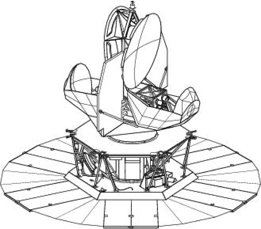
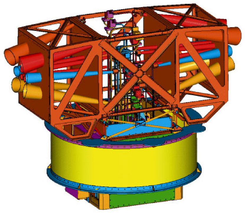
Figure 1: Left: A line drawing of the MAP satellite. Two back-to-back shaped Gregorian telescopes focus incident radiation onto the feeds which are located directly below the primary mirrors. The large circular disk at the bottom shields the telescopes from sunlight. The diameter of the disk is 5.1 m and the satellite is 3.6 m high. Right: The “focal plane assembly” (FPA) that houses the feeds. There are ten feeds on each side. The central area of the FPA houses the microwave receivers.

The accuracy with which MAP aims to measure the CMB anisotropy signal is $\sim 1\mu K$, much smaller than the brightest objects in the microwave sky. Thus, it is crucial to understand all contributions to the measured flux. The MAP feeds were designed to have a beam size of $\approx 9\deg$ full width at half maximum (FWHM), illuminating the secondary mirrors roughly equally in all bands. Beam spill past the secondary leads to an unfocused lobe offset from the main beam. If the secondary subtended only a cone of half angle $20\deg$ as viewed from a feed, the Galactic center in Q-band would contribute a $>130\ \mu$K signal directly through a feed as it was illuminated from over the rim of the secondary. The need for properly shielding and directing the feed response is clear. From the center of the focal plane, the perimeter of the secondary is $40\deg$ from the primary optical axis. The edge-taper on the secondary (ratio of the intensity at the edge to the peak value in the middle) is $<-50~{}$dB for all bands. Just as important as the shielding is the confidence that the far off-axis response of the feeds is understood so that firm limits may be placed on contamination. MAP’s primary beams are between $0\fdg 2$ and $1\deg$ in FWHM though they are not Gaussian. The interplay between the feed response and that of the full optical system is discussed in a companion paper Page et al. (2003).

2 Principles and Design of MAP’s Corrugated Feeds

The purpose of the MAP feeds is to smoothly transform a single circular TE₁₁ mode in the OMT into a hybrid HE₁₁ mode in the feed’s skyward aperture. The resulting beam is, as nearly as possible, cylindrically symmetric, linearly polarized and Gaussian in profile.

We may think of the feed in four separate sections. First, the input aperture (“input”) couples the feed to its OMT. This section is characterized by an input diameter and a short section of cylindrical guide. Second, the throat transforms the TE₁₁ mode in the circular guide into the hybrid mode HE₁₁. This section is characterized by $\sim 10$ grooves ranging from $\lambda/2$ to $\lambda/4$ deep. The third is the corrugated waveguide that propagates the hybrid mode. This section is characterized by grooves of depth $\lambda/4$, and may be conical or profiled. (The radius of a profiled horn grows nonlinearly along its length.) The fourth is the output which launches the hybrid mode. The output is characterized by a diameter and profile that can be shaped del Rio et al. (1996) to fine tune the beam.

The input diameter is chosen to impedance match the standard waveguide sizes and circular waveguide over the band. In particular, we match the cutoff wavelength of the rectangular waveguide TE₁₀ mode to the cutoff wavelength of the circular guide TE₁₁ mode and set $d_{input}=2a_{0}(1.841/\pi)$, where $a_{0}$ is the broad-wall dimension of the waveguide. Consequently, the circular waveguide impedance for TE₁₁ matches the wave impedance for TE₁₀ in rectangular waveguide: Z${}_{TE_{10}}$ = $\eta k/k_{g}=~{}$ Z${}^{circ}_{TE_{11}}$. Here $k$ is the free-space wavenumber, $k_{g}$ is the guide wavenumber, and $\eta$ is the wave impedance for a plane wave. This practice was followed successfully in Wollack et al. (1997).

The throat performs two separate functions: it matches the impedance of the smooth circular input waveguide to the grooved section of the horn, and ideally it transforms a TE₁₁ mode into a HE₁₁ mode. The feed throat design follows the work of Zhang (1993). A sample horn throat is shown in Figure LABEL:mode_form.

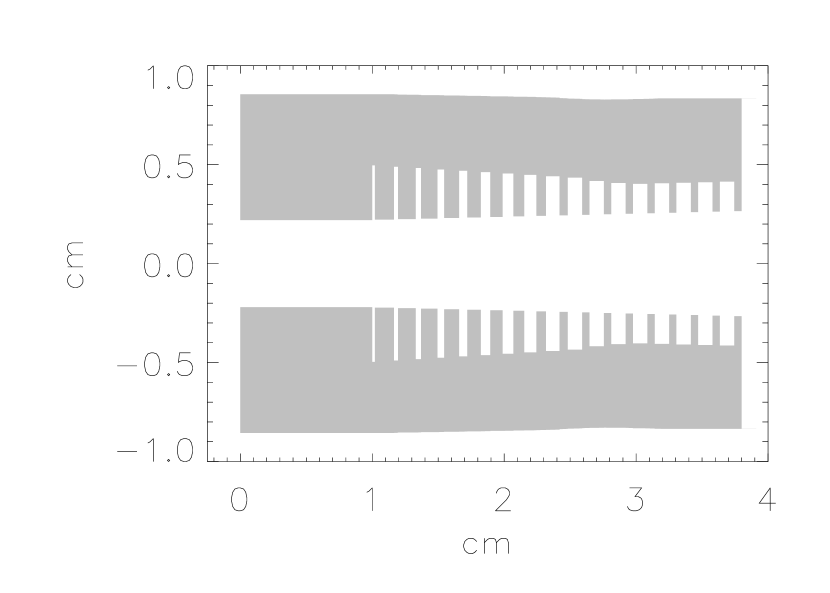
Figure 2: The mode-forming section of a V-band horn with center frequency 60 GHz. The rightmost six grooves are $\lambda/4$ deep. The OMT bolts onto the left side, and supplies a right-traveling TE₁₁ mode. The 1 cm long section of cylindrical waveguide ensures that the TE₁₁ is well established. Full groove patterns for all bands are available on request.

Once the HE₁₁ mode is formed, the corrugated horn expands adiabatically outward, stretching the mode to fill a larger cylinder, while maintaining its polarization, symmetry, and field pattern. The goal is to flare the horn to shape the HE₁₁ mode into a nearly Gaussian shape with a small cross-polar component. As the feed flares, the axial wavenumber $k_{g}\to k_{0}$, the free space value, inside the $\lambda/4$ corrugated waveguide, so propagating fields experience only a small discontinuity at the end of the feed. Accordingly, the propagating mode does not reflect from the skyward aperture, nor does it significantly diffract around the feed edges. (The edge currents, which are proportional to the edge fields, are close to zero.) The mode detaches as though it were already traveling through free space.

The output diameter of the feed was set following Touvinen (1992) to produce a $\approx 9\deg$ full width at half maximum ($\theta_{fwhm}$) beam. The aperture field for the HE₁₁ mode is given by $E_{x}(\rho)=0,\quad E_{y}(\rho)=A{J_{0}}^{\top}(k_{c}\rho)e^{-ik\rho^{2}/2R_{\rm sl}}\ ,$ where ${J_{0}}^{\top}(x)=J_{0}(x)$ for $x\leq\xi$ and 0 otherwise. Here $\xi\approx 2.405$ is the first zero of $J_{0}$, and $k_{c}=\xi/a$ where $a$ is the aperture radius, distinct from $R_{\rm sl}$, the effective slant length of the cone.

To first order in the far field, the emitted beam is Gaussian:
$E(\theta,z)\approx A\cos\theta e^{-\sin^{2}\theta(kw_{0}/2)^{2}}e^{-ikz}\ ,$ where $z$ is the direction along the axis of the feed, $\theta$ is the angle away from the $z$ axis, and $w_{0}=\zeta a/\sqrt{1+\zeta^{4}(ka^{2}/2R_{\rm sl})^{2}}$ is a virtual beam waist size. The constant, $\zeta\approx 0.6436$, is a dimensionless and numerically determined by maximizing power in the fundamental Gaussian mode. For a narrow beam, the full width at half maximum is thus $\theta_{fwhm}\approx 2{\sqrt{2\ln 2}\over kw_{0}}.$ These considerations led to the specification of the aperture, though in the final design the aperture diameter was optimized.

The final horns are shaped as in Figure LABEL:horns. Due to geometric constraints from the fairing diameter and receiver assembly, all the feeds are nearly the same length. This required lengthening the Q, V and W band feeds beyond their natural conical length Thomas (1978) and cosine-profiling the K-band feed Mahoud (1983) to shorten it from its natural conic length. In addition to satisfying the length constraints, the Q, V, and W feeds are flared del Rio et al. (1996) to enhance the Gaussanity of the beam.

Some microwave feeds have choke grooves around the rim of the aperture. These were not necessary for MAP because the gain of the feeds is high ($\approx 26~{}$dB); the coupling of two side-by-side feed horns is predicted to be $<-100$ dB. With the full optical system assembled, the measured coupling between pairs of the four feeds in W band is $-75$ dB to $-80$ dB. This cross talk is due to reflections from the microwave shielding around the secondary, not to direct feed-to-feed coupling, and is still too small to generate any observable correlations between radiometers.

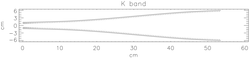
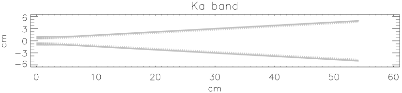
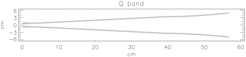
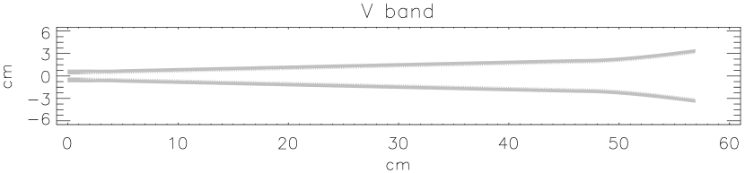
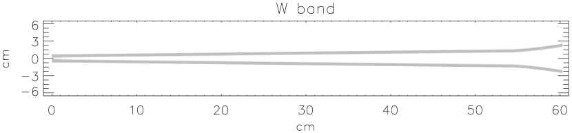
Figure 3: Profiles of the MAP feed horns. The corrugations are clearly visible in the K-band feed and less visible in the others due to printing resolution. The shapes and precise dimensions are available upon request.

3 Fabrication of the Feeds

Table 1 shows the specifications for each band. The K and Ka band horns are turned from single blocks of 7075 aluminum. The higher frequency MAP feed horns: Q, V, and W bands, are long and narrow and are therefore fabricated in 3, 4, and 5 short sections respectively which bolt together. Each joint is placed on a groove boundary, so the two sections mate to complete the groove; a cylindrical lock-and-key pattern forces these flanges to self-align, as in Figure LABEL:joint. The section closest to the OMT is electro-formed in copper, and then gold plated. The remaining, wider sections are machined from 7075 aluminum because of its machineability. Each machined section went through a regimen of repeated inspection, 380 K to 77 K thermal cycles, ultrasound, air jet and methanol cleaning to remove metal chips. After cleaning the measured interior surface roughness is $0.7\ \mu$m RMS.

Table 1: Dimensions of the MAP feeds

Band	WR	$\nu$	$\nu_{gv}$	Length	Apt.	Mass	Throat	$N_{gv}$	$N_{s}$	$\theta_{fwhm}$	Gain
		GHz	GHz	cm	cm	gm	cm			deg	dBi
K	42	19.5–25	22.0	53.64	10.9374	1010	1.2496	116	1	10.1–7.7	24.9–28.1
Ka	28	28–37	25.9	54.21	8.9916	650	0.8336	169	1	8.9-6.7	26.1–29.1
Q	22	35–46	32.5	56.76	8.9878	615	0.6680	217	3	7.8-6.0	27.3–30.8
V	15	53–69	49.1	56.96	5.9890	325	0.4408	329	4	8.8-7.4	26.0–28.8
W	10	82–106	90.1	60.33	3.9916	214	0.2972	533	5	9.7-8.3	25.0–27.2

Diameters are given for the feed length, aperture and throat. $N_{s}$ is the number of separate machined pieces from which the horn is assembled. Standard waveguide bands were chosen to minimize fabrication and testing costs for the microwave receivers. $\nu_{gv}$ is the frequency for which the horn groove depth is $\lambda/4$ (sometimes called the hybrid frequency). The antenna beam width range and gains run from the lowest to highest frequencies in the band. (The number shown is the average of E and H-plane FWHM.)

Figure 4: A joint between two sections of a W-band feed. The machining tolerance is 40 $\mu$m on the grooves and 5 $\mu$m on the joints. The flange design axially constrains the mating of the two section. Once the press fit joint is properly seated and the screws uniformly torqued, the joint is robust.

The final stage of fabrication consists of joining the feed sections. Especially at high frequencies, each joint must be mated carefully; a gap or misalignment can cause reflections or launch unwanted modes. At W-band, the feed joints are so critical and sensitive to proper mating that the feeds were assembled joint by joint, with the feed attached to a network analyzer. Spikes in the reflection spectrum often showed otherwise invisible flaws in the section-to-section mate. This procedure entwined the processes of building the horns and of measuring their properties.

4 Detailed predictions of antenna patterns, reflections and loss

Once the horn design is known in detail, it is possible to calculate its beam pattern precisely. MAP uses a commercial program called CCORHRNYRS Associates . The algorithm solves Maxwell’s equations exactly within the feed James (1981), so its predictions are correct up to manufacturing defects. The result is a complete solution for the radiation field inside the feed. The full pattern at any point in space can then be computed from a spherical wave expansion of the field in the skyward aperture. As the secondary mirrors are not in the far field of the feeds ($>8a^{2}/\lambda$) such an expansion is required for accurate predictions of the full telescope pattern.

The same model may be used to compute the loss in the feed Clarricoats & Olver  1994 . In the W-band feeds, most of the loss comes from the tenth through fiftieth grooves in the horn, counting from the OMT aperture. At 293 K, for a gold surface ($\sigma=4.4\times 10^{7}~{}$mhos/m ), the calculated emission temperature is 5.1 K corresponding to an emissivity of $\epsilon={\rm T_{emis}/T_{phys}}=0.017$. If one approximates the throat as a 1 cm length of round guide followed by corrugated waveguide with grooves of depth $\lambda/4$, the computed emissivity Clarricoats & Olver  1994 is 0.008, a factor of two less than for the full calculation.

5 Measurements and Modeling of the Beam Patterns.

The antenna patterns of all MAP’s feeds were measured before installation into the satellite. While a manufacturing flaw will typically alter both the horn’s reflection spectrum and its beam pattern, it is quite possible for a scratch, metal chip, or miscut groove to alter one but not the other.

Princeton’s mathematics department is housed in Fine hall tower, a thin rectangular building $\sim$ 50 m tall. From the roof of the physics department, $\sim$ 70 m away, the tower is silhouetted alone against empty sky, which makes it an ideal place for a microwave source. We mount sources, one for each band ranging from 140 to 800 mW in strength, on top of the tower and direct their radiation, modulated at 1 kHz, at the roof of the physics building with standard-gain horns. As a result, a $\sim$ 5m wide region of the physics department roof is illuminated with uniform, monochromatic, unidirectional microwave radiation.

Both the E- and H-planes are measured with both vertical and horizontal scans. For the E-plane, first the E-plane co-polar response is determined, for example with a vertical scan. Next the source polarization is rotated 90 degrees and the opposite port on the OMT is selected and the measurement repeated, yielding another E-plane beam pattern but in a horizontal scan. The H-plane is measured similarly. This double-scanning technique served to isolate unwanted geometrical features on the range. For instance, any reflection that interferes with the H-plane beam pattern when one scans sideways would be unlikely to contribute when the scan is vertical (and even less likely to distort the antenna pattern in the same way).

Figure 5: E and H-plane beam patterns for five feed horns. In these plots, the solid lines are measured responses and the dashed curves are predicted beam patterns, calculated as in section 4. With the exception of W-band, these beams were mapped in two stages: a first, inner map of the beam peak without an RF amplifier, and a second, outer map of the side-lobes with the amplifier installed. These measurements are matched at their overlaps. Each plot here overlays two scans: one vertical with the feed scanning from the sky (positive angles) down into the roof (negative angles), and one horizontal with the feed scanning from the source to the horizon at a cross elevation of about $80\deg$. Discrepancies in the far side-lobes of these scans are evidence of reflections in the range. The little “legs” at -30 dB result from the noise floor of the main beam scan.

One pair of antenna patterns from each band is shown in Figure LABEL:patterns, together with the beam pattern predictions for that horn design at that frequency. The peak response of each beam has been normalized; there is not an absolute calibration of the feed gain.

The agreement between the theoretical and measured patterns is excellent, particularly in the central lobe. A disagreement indicates an imperfection in the horn. In Wf4, for example, the E-plane plot shows a slight broadening near the beam peak, which indicates a second small amplitude mode propagating through the feed. (This discrepancy was judged not large enough to disqualify the horn from flight.)

Figure 6: Two deep sidelobe measurements of a Ka band horn. Beyond 150 degrees, the horn looks below the horizon, and sees reflections from the ground. Below -25 degrees, another unwanted reflection dominates.

The feed’s receiving pattern when it looks far away from the source, at angles $>90\deg$ is also measured. The predicted antenna pattern is extremely low in this region ($-60$ to $-90$ dB below beam peak), so the measurement is more difficult, and sensitive to reflections. Because the CMB anisotropy signal is so faint compared with the brightest objects in the sky, we are compelled to understand this ordinarily ignorable section of the antenna pattern. One such measurement of a Ka-band horn is shown in Figure LABEL:ka_deep. Beyond about $90\deg$, there is no longer close agreement between the predicted and measured beam patterns. This makes sense, when the horn is turned further than $90\deg$ away from the source there is an additional conducting boundary, the outside of the horn, which becomes important, and which is not included in the predictions. In terms of geometric optics, once the horn rotates beyond $90\deg$ from the source, its aperture is in the shadow of the horn itself. (It is tempting to explain the low signal around $90\deg$ in Figure LABEL:ka_deep purely in terms of this shadow, but that is an oversimplification. In contrast, the E-plane scan is higher than predictions in the same region.) The feed’s outer surface is not included in the beam predictions, though, because the response was measured to be small, we know modifications to the model are unnecessary for our purposes.

The predicted strength of the cross-polar antenna response varies strongly across the band for each feed. In each band, the cross-polar antenna pattern is four-lobed, with the four lobes together illuminating an angular region comparable to the co-polar beam area. The predicted ratios of maximum cross-polar antenna gains to maximum copolar gains are: in K-band, -31 dB, in Ka-band -39 dB, in Q-band -39 dB, in V-band -33 dB, and in W-band -44 dB. In other words in K-band the strongest cross-polar pickup for a source in the band is 31 dB weaker than the peak copolar response at the same frequency. Cross-polar pickup depends strongly on frequency within each band; the reported cross-polar sensitivity is the maximum value for each feed. Manufacturing defects will tend to increase any cross-polar contamination.

For MAP, the feed’s cross-polar signal is dominated by mode-mixing in the OMT in all but K band Jarosik et al. (2003). The OMTs misdirect polarized radiation at $<-25~{}$ dB level, while the cross-polarization in the feeds is predicted to be below $<-30~{}$ dB. As the OMTs limit the polarization separation, there was no reason to probe the cross-polarized response of the horns deeper than OMT level. In K and Ka bands, the configuration of the optics has a greater affect on the cross-polar response than either the feed or the OMT. In terms of CMB measurements, even the polarization mixtures induced by the OMTs will be an ignorably small contribution to the error in MAP’s polarization measurement.

After the individual feed measurements, the feeds were installed in MAP’s focal planes and the entire optical system (with reflectors) was mapped in an 5706 electromagnetic anechoic chamber facility at NASA/GSFC called the GEMAC. The GEMAC is based on MI Technologies positioners and 5706 antenna system. The receivers and microwave sources are made by Anritsu. The GEMAC can map all MAP’s bands with 1 kHz resolution plane wave source to -50 dB from the peak response over almost 2$\pi$ sr with an absolute accuracy of $<0.5$ dB. The resulting agreement between the predicted and main beam response (Page 2003 et al.), including absolute gain, is further evidence that the feeds met specifications. In all cases, the Princeton and GEMAC beam profiles were consistent.

6 Measurements of the reflections

The MAP feeds have $\leq-25$ dB reflections across their bands, as measured with a Hewlett Packard 8510C 1-110 GHz network analyzer. It is necessary to connect the horn to the network analyzer via a straight rectangular-to-circular waveguide transition (rather than an OMT with one arm terminated), since the OMTs typically have much higher reflection coefficients than do the feeds. The OMTs are characterized separately. As MAP is a differential instrument, an imbalance in its inputs leads to an offset in which one input always appears hotter. This offset is present even if there is no celestial signal. A large offset, in turn, leads to a higher $1/f$ noise knee in the radiometer Jarosik et al. (2003). Reflections from the OMT/feed assemblies can produce offsets through two effects. In the first, noise emitted from the HEMT amplifiers’ inputs is reflected by the OMT/feed back into the radiometer with slightly different magnitudes. The offset from this effect is roughly $T_{offset}\sim(T_{amp}-T_{ant})(\alpha_{A}-\alpha_{B})$ where $T_{amp}$ is the effective temperature of the noise power emitted from the input of the radiometers HEMT amplifiers, and $\alpha_{A}$ and $\alpha_{B}$ are the power reflections coefficients for the OMT/feed assemblies connected to the two inputs, and $T_{ant}\approx 3~{}$K. For W-band, $T_{amp}\approx 100K$. If $\alpha_{A}$ and $\alpha_{B}$ are both $\approx-25~{}$dB and are matched to about 10%, $T_{offset}\approx 50~{}$mK. In the second effect, the reflections produce coherent crosstalk between the two HEMT amplifiers. Ideally, each of the two input HEMT amplifiers sees the sum of two incoherent radiation fields, one from each side of the satellite. When the input noise from one HEMT reflects off the OMTs/feeds, it reenters both arms of the differential receiver coherently and produces an offset of $T_{offset}\sim({T_{amp}-T_{ant})\sqrt{\alpha}\beta\gamma}\approx 0.2~{}{\rm K}$ where $\beta\approx 0.2$ is a correlation coefficient that indicates the degree to which the noise emitted from the input of the HEMT is correlated to the amplified noise at the output of the amplifier, $\alpha\approx\alpha_{A}\approx\alpha_{B}$, and $\gamma\approx 0.15$ (W-band) is a factor to allow for the bandwidth averaging of the effect from the different path lengths the signals take before being recombined.

Samples of the measured reflection strengths are shown in Figure LABEL:reflections together with predictions. The network analyzer measures a single mode and was calibrated for a rectangular waveguide. The feed reflections are an extremely sensitive indicator of manufacturing defects.

Figure 7: Predicted and measured reflected power for a selection of the MAP feed horns. The measured and predicted reflections are solid and dashed respectively. The reflected power is $10\log_{10}|S_{11}|^{2}$ where $S$ is the scattering matrix. The vertical dotted lines mark MAP radiometer band edges, and the horizontal dashed line provides a reference at -30 dB. The measured reflection strengths show the combined effect of the rectangular-to-circular waveguide transition and the feed. (Predictions include only the feed.) In particular, the small regular oscillations in all the measured reflections correspond to the rectangular-to-circular transition length. In K band, the return loss is dominated by the transition; in W band it is dominated by feed. Feed KaF2 has a shallow spiral scratch inside its throat, an accident of fabrication. (KaF2 was not installed on the satellite.)

7 Measurements of the Loss

The loss in an ideal corrugated feed Clarricoats, Olver, & Chong (1975) is small and often negligible; consequently there are not many measurements of it. If the loss is not balanced between the two sides of the differential radiometer, the output will have an offset. If the temperature of the feeds varies significantly, the offset will vary and possibly introduce a signal that confounds the celestial signal. For loss in the feeds, the offset between the $A$ and $B$ sides is $T_{offset}\approx\epsilon_{A}T_{A}-\epsilon_{B}T_{B}$ where $\epsilon_{A}$ and $\epsilon_{B}$ are the feed emissivities. For example, if $T_{offset}=1~{}$K with the feeds at $T_{A}=T_{B}=100$ K, the temperature of the feeds must be stable to 0.1 mK to avoid spurious signals $>1~{}\mu$K. The spacecraft instrumentation can detect instability at this level.

The emissivity of a room temperature feed was measured Bradley (1998) to be $\epsilon=0.11$ at 90 GHz, well above the modeled emissivity of $\epsilon=0.017$. The measurement was made by uniformly heating a feed that was thermally isolated from a stabilized 90 GHz receiver. The emission temperature of the feed was compared to the emission temperature of a stabilized load at a variety of feed temperatures.

During the cold testing (100 K) of the MAP receivers plus feed horns, it was found that in one case an offset of $T_{offset}=2.5~{}$K could be clearly attributed to imbalanced emission from the feeds corresponding to $\epsilon_{a}-\epsilon_{B}=0.025$. If the loss were metallic, one would expect the emissivity of one feed to be $\epsilon=0.057$ at 100 K and the difference between two feeds to be significantly less than this. The offending feed was replaced and the amplitude of the offset was reduced. Based on the differential measurements, the loss in other feeds was considered acceptably low; however, we cannot be certain that the theoretical performance was achieved for any feeds because the measurement is intrinsically differential. The in-flight performance will be addressed in a future paper.

The large emissivities of the test feed and the “flight feed” that was replaced were traced to improper gold plating that became clearly evident after one of the electroformed feed sections was sliced open. To guard against deterioration of the other electroformed feed tails, they were continuously purged with nitrogen until launch.

8 Conclusion

The nature of CMB anisotropy, microkelvin fluctuations in a sky containing sources many orders of magnitude brighter, requires close attention to properties of optical elements of any CMB telescope. Ordinarily ignorable features, particularly far off-axis antenna pickup, can significantly effect measured temperatures. For each optical component of MAP, it is crucial to understand the full antenna pattern, emissivity, and any backscatter native to that element.

The MAP feeds produce near-Gaussian beams with low reflections across their bands. The measured beam patterns match the predictions strikingly well; in some cases measurement and theory agree to $-80~{}$dB. No significant discrepancy between the predicted and measured beam patterns was seen at angles $<90\deg$ for a well manufactured feed; beyond 90 degrees, the calculation neglects an important boundary term. Similar accuracy was not needed for the reflection predictions as reflections are dominated by the OMT. However, measurement confirm that the horn reflection spectra are low enough for MAP’s purposes. The feed cross-polar pattern is computable and negligible. For MAP the cross-polar pattern is dominated by the OMT and reflector configuration. The feed loss is low in most cases, but a manufacturing problem led to a demonstrably higher than expected emissivity in two out of fourteen electroformed W-band feed tails.

We have shown that corrugated feeds can be manufactured in a variety of shapes and that with detailed attention to the manufacture, the theoretical performance may be achieved. Future missions will undoubtedly use corrugated structures because of their many benefits.

9 Acknowledgments

The design, building and testing of the MAP feeds took over two years. The Princeton machine shop was invaluable in this program, especially Glenn Atkinson who spent a year on machining alone. Ken Stewart and Steve Suefert kept NASA/GSFC’s GEMAC indoor beam mapping facility mapping for weeks at a time. Charles Sule inspected all of the feeds and Alysia Marino assisted in the measurements. The modeling of the feeds was made possible by assistance and code from YRS Associates: Yahya Rahmat-Samii, Bill Imbriale, and Vic Galindo. Of particular note, YRS Associates derived the groove dimensions, feed shapes, and computed the fed emissivity. This research was supported by the MAP Project under the NASA Office of Space Science. More information about MAP may be found at http://map.gsfc.nasa.gov.

References

- Bennett et al. (2003) Bennett, C. et al. 2003, Accepted for publication ApJ
- Bradley (1998) Bradley, S. 1998, An Estimation of the Emissivity of a W-band Feed Horn and Orthomode Transducer, Senior thesis, Princeton
- (3) Clarricoats, P. J. B. and Olver, A. D. 1984 Corrugated horns for microwave antennas, Peter Peregrinus Ltd.
- Clarricoats, Olver, & Chong (1975) Clarricoats, Olver, Chong, 1973, Proc. IEE-London, 122 11
- del Rio et al. (1996) del Rio, C., Gonzalo, R. & Sorolla, M. 1996, Proceedings of the ISAP ’96, Chiba, Japan
- James (1981) James, G. L. 1981, IEEE Trans. Microwave Theory and Techniques MTT-29 1059
- Jarosik et al. (2003) Jarosik, N. et al. 2003, ApJS145, Accepted.
- Jones (1998) Jones, W. C. 1998, Microwave Anisotropu Probe Feed Antenna Design Verification Senior thesis, Princeton, 1998
- Mahoud (1983) Mahoud, S. F. 1983, IEEE Proc. 130 415
- Page et al. (2003) Page, L. et al., 2003, ApJ585, Accepted.
- Thomas (1978) Thomas, B. M. 1978, IEEE Trans. on Antennas and Propagation, AP-26 367
- Touvinen (1992) Touvinen, J. 1992, IEEE Trans. Antennas and Propogation, 40 391
- Wollack (1997) Wollack, E. J., Devlin, M. J., Jarosik, N., Netterfield, C. B., Page, L., & Wilkinson, D. 1997, ApJ476 440
- (14) YRS associates, rahmat@ucla.edu
- Zhang (1993) Zhang, X. 1993, IEEE Trans. Microwave Theory and Techniques, 41 1263