The Microwave Anisotropy Probe (MAP ) Mission

Abstract

The purpose of the MAP mission is to determine the geometry, content, and evolution of the universe via a 13 arc-min full-width-half-max (FWHM) resolution full sky map of the temperature anisotropy of the cosmic microwave background radiation with uncorrelated pixel noise, minimal systematic errors, multifrequency observations, and accurate calibration. These attributes were key factors in the success of NASA’s Cosmic Background Explorer (COBE) mission, which made a $7^{\circ}$ FWHM resolution full sky map, discovered temperature anisotropy, and characterized the fluctuations with two parameters, a power spectral index and a primordial amplitude. Following COBE considerable progress has been made in higher resolution measurements of the temperature anisotropy. With 45 times the sensitivity and 33 times the angular resolution of the COBE mission, MAP will vastly extend our knowledge of cosmology. MAP will measure the physics of the photon-baryon fluid at recombination. From this, MAP measurements will constrain models of structure formation, the geometry of the universe, and inflation. In this paper we present a pre-launch overview of the design and characteristics of the MAP mission. This information will be necessary for a full understanding of the MAP data and results, and will also be of interest to scientists involved in the design of future cosmic microwave background experiments and/or space science missions.

1 INTRODUCTION

The existence of the cosmic microwave background (CMB) radiation (Penzias & Wilson, 1965), with its precisely measured blackbody spectrum (Mather et al., 1999, 1994, 1990; Fixsen et al., 1996, 1994; Gush et al., 1990), offers strong support for the big bang theory. CMB spatial temperature fluctuations were long expected to be present due to large-scale gravitational perturbations on the radiation (Sachs & Wolfe, 1967), and due to the scattering of the CMB radiation during the recombination era (Silk, 1968; Sunyaev & Zeldovich, 1970; Peebles & Yu, 1970). Detailed computations of model fluctuation power spectra reveal that specific peaks form as a result of coherent oscillations of the photon-baryon fluid in the gravitational potential wells created by total density perturbations, dominated by non-baryonic dark matter (Bond & Efstathiou, 1984, 1987; Wilson & Silk, 1981; Sunyaev & Zeldovich, 1970; Peebles & Yu, 1970). For a given cosmological model the CMB anisotropy power spectrum can now be calculated to a high degree of precision (Hu et al., 1995; Zaldarriaga & Seljak, 2000), and since the values of interesting cosmological parameters can be extracted from it, there is a strong motivation to measure the CMB power spectrum over a wide range of angular scales with accuracy and precision.

The discovery and characterization of CMB spatial temperature fluctuations (Smoot et al., 1992; Bennett et al., 1992; Wright et al., 1992; Kogut et al., 1992) confirmed the general gravitational picture of structure evolution. The COBE 4-year full sky map, with uncorrelated pixel noise, precise calibration, and demonstrably low systematic errors (Bennett et al., 1996; Kogut et al., 1996a; Hinshaw et al., 1996; Wright et al., 1996b; Gorski et al., 1996) provides the best constraint on the amplitude of the largest angular scale fluctuations and has become a standard of cosmology (i.e., “COBE-normalized”). Almost all cosmological models currently under active consideration assume that initially low amplitude fluctuations in density grew gravitationally to form galactic structures.

At the epoch of recombination, $z\sim 1100$, the scattering processes that leave their imprint on the CMB encode a wealth of detail about the global properties of the universe. A host of ground-based and balloon-borne experiments have since aimed at characterizing these fluctuations at smaller angular scales (Dawson et al., 2001; Halverson et al., 2001; Hanany et al., 2000; Leitch et al., 2000; Wilson et al., 2000; Padin et al., 2001; Romeo et al., 2001; de Bernardis et al., 2000; Harrison et al., 2000; Peterson et al., 2000; Baker et al., 1999; Coble et al., 1999; Dicker et al., 1999; Miller et al., 1999; de Oliveira-Costa et al., 1998; Cheng et al., 1997; Hancock et al., 1997; Netterfield et al., 1997; Piccirillo et al., 1997; Tucker et al., 1997; Gundersen et al., 1995; de Bernardis et al., 1994; Ganga et al., 1993; Myers et al., 1993; Tucker et al., 1993).

Multiple groups are presently developing instrumentation and techniques for detection of the polarization signature of CMB temperature fluctuations. At the time of this writing, only upper bounds on polarization on a variety of angular scales have been reported (Partridge et al., 1997; Sironi et al., 1998; Torbet et al., 1999; Subrahmanyan et al., 2000; Hedman et al., 2001; Keating et al., 2001).

Experimental errors from CMB measurements can be difficult to assess. While the nature of the random noise of an experiment is reasonably straightforward to estimate, systematic measurement errors are not. None of the ground or balloon-based experiments enjoy the extent of systematic error minimization and characterization that is made possible by a space flight mission (Kogut et al., 1992, 1996a).

In addition to the systematic and random errors associated with the experiments, there is also an unavoidable additional variance associated with inferring cosmology from a limited sampling of the universe. A cosmological model predicts a statistical distribution of CMB temperature anisotropy parameters, such as spherical harmonic amplitudes. In the context of such models, the true CMB temperature observed in our sky is only a single realization from a statistical distribution. Thus, in addition to experimental uncertainties, we account for cosmic variance uncertainties in our analyses. For a spherical harmonic temperature expansion $T(\theta,\phi)=\sum_{\ell m}a_{\ell m}Y_{\ell m}(\theta,\phi)$, cosmic variance is approximately expressed as $\sigma(C_{\ell})/C_{\ell}\approx\sqrt{2/(2\ell+1)}$ where $C_{\ell}=<|a_{\ell m}|^{2}>$. Cosmic variance exists independent of the quality of the experiment. The power spectrum from the 4-year COBE map is cosmic variance limited for $\ell\lesssim 20$.

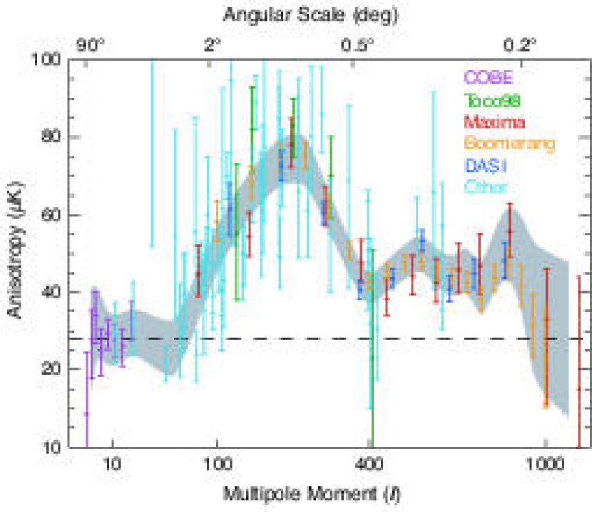
Figure 1: The angular power spectrum indicates the state of CMB anisotropy measurements at the time of the MAP launch. The grey $2\;\sigma$ band denotes the uncertainty in a combined CMB power spectrum from recent anisotropy experiments. (Boomerang 2000 results are omitted in favor of Boomerang 2001 results.)

Fig. 1 shows the state of CMB anisotropy power spectrum research at about the time of the MAP launch, by combining the results of many recent measurement efforts. The width of the grey error band is determined by forcing the $\chi^{2}$ of the multi-experiment results to be unity. Conflicting measurements are thus effectively handled by a widening of the grey band. Although the grey band is consistent with the set of measurements, its absolute correctness is still entirely dependent on the correctness of the values and errors claimed by each experimental group.

2 COSMOLOGICAL PARADIGMS

The introduction of the inflation model (Guth, 1981; Sato, 1981; Linde, 1982; Albrecht & Steinhardt, 1983) augmented the big bang theory by providing a natural way to explain why the geometry of universe is nearly flat (the “flatness problem”), why causally separated regions of space share remarkably similar properties (the “horizon problem”), and why there is a lack of monopoles or other defects observed today (the “monopole problem”). While the original inflation model made strong predictions of a nearly perfectly flat geometry and equal gravitational potential fluctuations at all spatial scales, inflationary models have since been seen to allow for a wide variety of other possibilities. In its simplest conception, the inflaton field that drives inflation is a single scalar field. More generally, a wide variety of formulations of the inflaton field are possible, including multiple scalar and non-minimally coupled scalar fields. Thus inflation is a broad class of models, including models that produce an open geometry, and models that deviate from generating equal gravitational potential fluctuation power on all spatial scales. The breadth of possible inflationary scenarios has led to the question of whether inflation can be falsified. CMB observations can greatly constrain which inflationary scenarios, if any, describe our universe.

In the simplest inflationary models, fluctuations arise from adiabatic curvature perturbations. More complicated models can generate isocurvature entropy perturbations, or an admixture of adiabatic and isocurvature perturbations. In adiabatic models the mass density distribution perturbs the local space-time curvature, causing curvature fluctuations up through superhorizon scales (Bardeen, Steinhardt & Turner, 1983). These are energy density fluctuations with a homogeneous entropy per particle. In isocurvature models the equation of state is perturbed, corresponding to local variations in the entropy. Radiation fluctuations are balanced by baryons, cold dark matter, or defects (textures, cosmic strings, global monopole’s, or domain walls). Fluctuations of the individual components are anticorrelated with the radiation so as to produce no net perturbation in the energy density. The distinct time-evolution of the gravitational potential between curvature and isocurvature models lead to very different predictions for the CMB temperature fluctuation spectrum. These fluctuations carry the signature of the processes that formed structure in the universe, and of its large-scale geometry and dynamics.

In adiabatic models, photons respond to gravitational potential fluctuations due to total matter density fluctuations to produce observable CMB anisotropy. The oscillations of the pre-recombination photon-baryon fluid are understood in terms of basic physics, and their properties are sensitive to both the overall cosmology and to the nature and density of the matter.

The following CMB anisotropy observables should be seen within the context of the simplest form of inflation theory (a single scalar field with adiabatic fluctuations) (Linde, 1990; Kolb & Turner, 1990; Liddle & Lyth, 2000): (1) an approximately scale-invariant spectral index of primordial fluctuations, $n\approx 1$; (2) a flat $\Omega_{0}=1$ geometry, which places the first acoustic peak in the CMB fluctuation spectrum at a spherical harmonic order $\ell\backsim 220$; (3) no vector component (inflation damps any initial vorticity or vector modes, although vector modes could be introduced with late-time defects); (4) Gaussian fluctuations with random phases; (5) a series of well-defined peaks in the CMB power spectrum, with the first and third peaks enhanced relative to the second peak (Hu & White, 1996); and (6) a polarization pattern with a specific orientation with respect to the anisotropy gradients.

More complex inflationary models can violate the above properties. Also, these properties are not necessarily unique to inflation. For example, tests of a $n=1$ spectrum of Gaussian fluctuations do not clearly distinguish between inflationary models and alternative models for structure formation. Indeed, the $n=1$ prediction predates the introduction of the inflation model (Harrison, 1970; Zeldovich, 1972; Peebles & Yu, 1970). Gaussianity may be the weakest of the three tests since the central limit theorem reflects that Gaussianity is the generic outcome of most statistical processes.

Unlike adiabatic models, defect models do not have multiple acoustic peaks (Pen, Seljak & Turok, 1997; Magueijo et al., 1996) and isocurvature models predict a dominant peak at $l\approx 330$ and a subdominant first peak at $l\approx 110$ (Hu & White, 1996). It is possible to construct a model that has isocurvature initial conditions with no superhorizon fluctuations that mimics the features of the adiabatic inflationary spectrum (Turok, 1997). This model, however, makes very different predictions for polarization-temperature correlations and for polarization-polarization correlations (Hu, Spergel & White, 1997). By combining temperature anisotropy and polarization measurements, there will be a set of tests that are both unique (only adiabatic inflationary models pass) and sensitive (if the model fails the test, then the fluctuations are not entirely adiabatic).

If the inflationary primordial fluctuations are adiabatic, then the microwave background temperature and polarization spectrum is completely specified by the power spectrum of primordial fluctuations, and a few basic cosmological numbers: the geometry of the universe ($\Omega_{0}$, $\Lambda_{0}$), the baryon/photon ratio ($\Omega_{b}h^{2}$), the matter/photon ratio ($\Omega_{m}h^{2}$), and the optical depth of the universe since recombination ($\tau$). If these numbers are fixed to match an observed temperature spectrum, then the properties of the polarization fluctuations are nearly completed specified, particularly for $l>30$ (Kosowsky, 1999). If the polarization pattern is not as predicted, then the primordial fluctuations can not be entirely adiabatic.

If a polarization-polarization correlation is found on the few degree scale, then a completely different proof of superhorizon scale fluctuations comes into play. Since polarization fluctuations are produced only through Thompson scattering, then if there are no superhorizon density fluctuations, there should be no superhorizon polarization fluctuations (Spergel & Zaldarriaga, 1997).

There are two types of polarization fluctuations: “E modes” (gradients of a field) and “B modes” (curl of a field). Scalar fluctuations produce only E modes, while tensor (gravity wave) and vector fluctuations produce both E and B modes. Inflationary models produce gravity waves (Kolb & Turner, 1990) with a specific relationship between the amplitude of tensor modes and the slope of the tensor mode spectrum. The CMB gravity wave polarization signal is extremely weak, with a rms amplitude well below 1 $\mu$K. The ability to detect these tracers in a future experiment will depend on the competing foregrounds and the ability to control systematic measurement errors to a very fine level. Unlike E modes, which MAP should detect, the B modes are not correlated with temperature fluctuations, so there is no template guide to assist in detecting these features. Also, the B mode signal is strongest on the largest angular scales where the systematic errors and foregrounds are the worst. The detection of B modes is beyond the scope of MAP ; a new initiative will be needed for a next-generation space CMB polarization mission to address these observations. MAP results should be valuable for guiding the design of such a mission.

3 MAP OBJECTIVES

The MAP mission scientific goal is to answer fundamental cosmology questions about the geometry and content of the universe, how structures formed, the values of the key parameters of cosmology, and the ionization history of the universe. With large aperture and special purpose telescopes ushering in a new era of measurements of the large-scale structure of the universe as traced by galaxies, advances in the use of gravitational lensing for cosmology, the use of supernovae as standard candles, and a variety of other astronomical observations, the ultimate constraints on cosmological models will come from a combination of all these measurements. Alternately, inconsistencies that become apparent between observations using different techniques may lead to new insights and discoveries.

A map with uncorrelated pixel noise is the most compact and complete form of anisotropy data possible without loss of information. It allows for a full range of statistical tests to be performed, which is otherwise not practical with the raw data, and not possible with further reduced data such as a power spectrum. Based on our experience with the COBE anisotropy data, a map is essential for proper systematic error analyses.

The statistics of the map constrain cosmological models. MAP will measure the anisotropy spectral index over a substantial wavenumber range, and determine the pattern of peaks. MAP will test whether the universe is open, closed, or flat via a precision measurement of $\Omega_{0}$, which is already known to be roughly consistent with a flat inflationary universe (Knox & Page, 2000). MAP will determine values of the cosmological constant, the Hubble constant, and the baryon-to-photon ratio (the only free parameter in primordial nucleosynthesis). MAP will also provide an independent check of the COBE results, determine whether the anisotropy obeys Gaussian statistics, check the random phase hypothesis, and verify whether the predicted temperature-polarization correlation is present. MAP will constrain the inflation model in several of the ways discussed in §2. Note that these determinations are independent of traditional astronomical approaches (that rely on, e.g., distance ladders or assumptions of virial equilibrium or standard candles), and are based on samples of vastly larger scales.

Table 1: MAP Mission Characteristics

Property	Configuration
Sky coverage	Full sky
Optical system	Back-to-Back Gregorian, 1.4 m $\times$ 1.6 m primaries
Radiometric system	polarization-sensitive pseudo-correlation differential
Detection	HEMT amplifiers
Radiometer Modulation	2.5 kHz phase switch
Spin Modulation	$0.464$ rpm $=$ $\sim 7.57$ mHz spacecraft spin
Precession Modulation	1 rev hr${}^{-1}=\sim 0.3$ mHz spacecraft precession
Calibration	In-flight: amplitude from dipole modulation, beam from Jupiter
Cooling system	passively cooled to $\sim 90$ K
Attitude control	3-axis controlled, 3 wheels, gyros, star trackers, sun sensors
Propulsion	blow-down hydrazine with 8 thrusters
RF communication	2 GHz transponders, 667 kbps down-link to 70 m DSN
Power	419 Watts
Mass	840 kg
Launch	Delta II 7425-10 on June 30, 2001 at 3:46:46.183 EDT
Orbit	$1^{\circ}-10^{\circ}$ Lissajous orbit about second Lagrange point, L2
Trajectory	3 Earth-Moon phasing loops, lunar gravity assist to L2
Design Lifetime	27 months = 3 month trajectory + 2 yrs at L2

Table 2: Band-Specific Instrument Characteristics

	K-Band	Ka-Band	Q-Band	V-Band	W-Band
Wavelength (mm)	13	9.1	7.3	4.9	3.2
Frequency (GHz)	23	33	41	61	94
Bandwidth (GHz)	5.5	7.0	8.3	14.0	20.5
Number of Differencing Assemblies	1	1	2	2	4
Number of Radiometers	2	2	4	4	8
Number of Channels	4	4	8	8	16
Beam size (deg)	0.88	0.66	0.51	0.35	0.22
System temperature, $T_{sys}$ (K)	29	39	59	92	145
Sensitivity (mK sec${}^{1/2})$	0.8	0.8	1.0	1.2	1.6

The high-level features of the MAP mission are described below and summarized in Tables 1 and 2. The mission is designed to produce a full ($>95$%) sky map of the cosmic microwave background temperature fluctuations with:

• $\approx 0.2^{\circ}$ angular resolution

• accuracy on all angular scales $>0.2\mbox{${}^{\circ}$}$

• minimally correlated pixel noise

• polarization sensitivity

• accurate calibration ($<0.5$% uncertainty)

• an overall sensitivity level of $\Delta T_{\rm rms}<20~{}\mu$K per pixel (for 393,216 sky pixels, $3.2\times 10^{-5}$ sr per pixel)

• systematic errors limited to $<5$% of the random variance on all angular scales

Systematic errors in the final sky maps can originate from a variety of sources: calibration errors, external emission sources, internal emission sources, multiplicative electronics sources, additive electronics sources, striping, map-making errors, and beam-mapping errors. The need to minimize the level of systematic errors (even at the expense of sensitivity, simplicity, cost, etc.) has been the major driver of the MAP design. To minimize systematic errors MAP has:

• a symmetric differential design

• rapid large-sky-area scans

• 4 switching/modulation periods

• a highly interconnected and redundant set of differential observations

• an L₂ orbit to minimize contamination from Sun, Earth, and Moon emission and allow for thermal stability

• multiple independent channels

• 5 frequency bands to enable a separation of galactic and cosmic signals

• passive thermal control with a constant Sun angle for thermal and power stability

• control of beam sidelobe levels to keep the Sun, Earth, and Moon levels $<1~{}\mu$K

• a main beam pattern measured accurately in-flight (e.g., using Jupiter)

• calibration determined in-flight (from the CMB dipole and its modulation from MAP’s motion)

• low cross-polarization levels (below -20 dB)

• precision temperature sensing at selected instrument locations

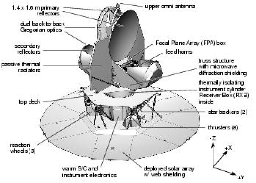
Figure 2: A view of the MAP Observatory is shown with several of the major constituents called out. The Observatory is 3.8 m tall and the deployed solar array is 5.0 m in diameter. The Observatory mass is 836 kg.

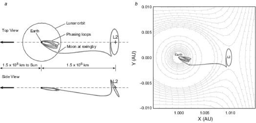
Figure 3: Views of MAP ’s trajectory to an orbit about L₂. MAP uses an L₂ orbit to enable passive cooling and to minimize systematic measurement errors. (a) Perspective views (from the North ecliptic pole and from within the ecliptic plane) of a typcal trajectory are shown in an Earth co-rotating coordinate system. An on-board reaction control (propulsion) system executes three highly elliptical “phasing loop” orbits about the Earth, which set up a gravity-assist lunar swing-by, and then a cruise to an orbit about the second Earth-Sun Lagrange point, L₂. (b) The co-rotating gravitational potential is shown. The break in contour lines represent a change of scale, where the gravitational potential near the Earth is much steeper than near L₂. Tick marks indicate the “down hill” side of each contour. The L₂ orbit provides a quasi-stable orbit in a saddle-shaped gravitational potential. This is a “Lissajous” rather than “halo” orbit since the Observatory is at a different position with a different velocity vector after each six-month loop.

4 HIGH-LEVEL SCIENCE MISSION DESIGN FEATURES

Fig. 2 shows an overview of the MAP Observatory. A deployable sun shield, with web blankets between solar panels, keeps the spacecraft and instrument in shadow for all nominal science operations. Large passive radiators are connected, via heat straps, directly to the High Electron Mobility Transistor (HEMT) amplifiers at the core of the radiometers. A (94 cm diameter $\times$ 33 cm length $\times$ 0.318 cm thick) gamma-alumina cylindrical shell provides exceptionally low thermal conductance (0.59 and 1.4 W m^-1 K^-1 at 80 K and 300 K, respectively) between the warm spacecraft and the cold instrument components. The back-to-back optical system can be seen as satisfying part of the requirement for a symmetric differential design. An L₂ orbit was required to minimize thermal variations while simplifying the passive cooling design, and to isolate the instrument from microwave emission from the Earth, Sun, and Moon. Fig. 3 shows the MAP trajectory, including its orbit about L₂.

Further systematic error suppression features of the MAP mission are discussed in the following subsections.

4.1 Thermal and Power Stability

There are three major objectives of the thermal design of MAP . The first is to keep all elements of the Observatory within nondestructive temperature ranges for all phases of the mission. The second objective is to passively cool the instrument front-end microwave amplifiers and reduce the microwave emissivity of the front-end components to improve sensitivity. The third objective is to use only passive thermal control throughout the entire Observatory to minimize all thermal variations during the nominal observing mode. While the first objective is common to all space missions, the second objective is rare, and the third objective is entirely new and provides significant constraints to the overall thermal design of the mission.

All thermal inputs to MAP are from the Sun, either from direct thermal heating or indirectly from the electrical dissipation of the solar energy that is converted in the solar arrays. Since both thermal changes and electrical changes are potential sources of undesired systematic errors, measures are taken to minimize both. The slow annual change in the effective solar constant is easily accounted for. Variations that occur synchronously with the spin period pose the greatest threat since they most closely mimic a true sky signal.

To minimize thermal and electrical variations the solar arrays maintain a constant angle relative to the Sun of $22.5\mbox{${}^{\circ}$}\pm 0.25\mbox{${}^{\circ}$}$ during CMB anisotropy observations at L₂. The constant solar angle, combined with the battery, provides for a stable power input to all electrical systems. Key systems receive further voltage referencing and regulation.

To further minimize thermal and electrical systematic effects, efforts are made to minimize variations in power dissipation. All thermal control is passive; there are no proportional heaters and no heaters that switch on and off (except for survival heaters that are only needed in cases of spacecraft emergencies, and the transmitter make-up heater, discussed below). The electrical power dissipation changes of the various electronics boxes are negligible.

Passive thermal control required careful adjustment and testing of the thermal blankets, radiant cooling surfaces, and ohmic heaters. A detailed thermal model was used to guide the development of a baseline design. Final adjustments were based on tests in a large thermal vacuum chamber, in which the spacecraft (without its solar panels) was surrounded by nitrogen-cooled walls and the instrument was cooled by liquid helium walls.

Radio frequency interference (RFI) from the transmitter poses a potential systematic error threat to the experiment. Thus, there is a motivation to turn the transmitter on for only the least amount of time needed to down-link the daily data. However, the power dissipation difference between the transmitter on and off states poses a threat to thermal stability. To mitigate these thermal changes, a $53~{}\Omega$ make-up heater is placed on the transponder mounting plate to approximately match the 21 Watt thermal power dissipation difference between the on versus off states of the transmitter. There are two transponders (one is redundant) and they are both mounted to the same thermal control plate. Both receivers are on at all times. The heater can be left on, except for the $\approx 40$ minute per day period that the transmitter must be used. Thus, there are two in-flight options for minimizing systematic measurement errors due to the transmitter. Should in-flight RFI from the transmitter be judged a greater threat than residual thermal variations, then the transmission time can be minimized and the make-up heater used. Alternately, should the residual thermal variations be the greater threat the transmitter can be left on continuously. The mission is designed such that either option is expected to meet systematic error requirements.

There are scores of precision platinum resistance thermometers (PRTs) at various locations to provide a quantitative demonstration of thermal stability at the sub-millikelvin level. The information from these sensors is invaluable for making a quantitative assessment of the level of systematic errors from residual thermal variations and could be used to make error corrections in the ground data reduction pipeline, if needed. The design is to make these corrections unnecessary and to use the sensor data only to prove that thermal variations are not significant.

4.2 Sky Scan Pattern

The sky scan strategy is critical to achieve minimal systematic effects in CMB anisotropy experiments. The ideal scan strategy would be to instantaneously scan the entire sky, and then rapidly repeat the scans so that sky regions are traversed from all different angles. Practical constraints, of course, limit the scan rate, the available instantaneous sky region, and the angles through which each patch of sky is traversed by a beam. For a space mission, increasing the scan speed rapidly becomes expensive: it becomes more difficult to reconstruct an accurate pointing solution; the torque requirements of on-board control components increase; and the data rates required to prevent beam smearing increase. The region of sky available for scanning is limited by the acceptable level of microwave pick-up from the Sun, Earth, and Moon.

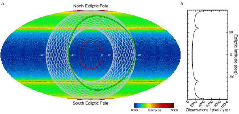
Figure 4: (a) A full sky map projection in ecliptic coordinates shows the number of independent data samples taken per year by sky position. Full sky coverage results from the combined motions of the spin, precession, and orbit about the Sun. The spin axis precesses along the red circle in 1 hour. When the spin axis is at the position of the blue “x” a feed pair traces the green circle on the sky in the 129 second spin period. The white circles indicate the results of the precession. Full sky coverage is achieved in six months as MAP orbits around the Sun (with the Earth). (b) The number of observations per pixel as a function of ecliptic latitude is shown for each full year of observations. The number of observations per pixel will vary by frequency band due to differing sampling rates, differing beam solid angles, and data flagging. The plot is illustrative; the MAP data must be used for exact sky sampling values.

It is possible to quantitatively assess the quality of a sky scanning strategy by computer simulation. Systematic errors are generated as part of an input to a computer simulation that converts time-ordered data to sky maps. The suppression factor of systematic error levels going from the raw time-ordered data into the sky map is a measure of the quality of the sky scanning strategy. A poor scanning strategy will result in a poor suppression factor. Our computer simulations show that the sky scanning strategy used by the COBE mission was very nearly ideal as it maximally suppressed systematic errors in the time-ordered data from entering the map. A large fraction of the full sky was scanned rapidly, consistent with avoiding a $60\mbox{${}^{\circ}$}$ full-angle cone in the solar direction. However, the Moon was often in and near the beam. This was useful for checks of amplitude and pointing calibration, but much data had to be discarded when contamination by lunar emission was significant. COBE, in its low Earth orbit, also suffered from pick-up of microwave emission from the Earth, also causing data to be discarded.

In its nominal L₂ orbit the MAP Observatory executes a compound spin (0.464 rpm) and precession (1 hr^-1), as shown in Figure 4. The MAP sky scan strategy is a compromise. While the MAP scan pattern is almost as good as COBE’s with regard to an error suppression factor, it is far better than COBE’s for rejecting microwave signals from the Sun, Earth, and Moon microwave signals.

The MAP sky scan pattern results in full sky coverage with some variation in the number of observations per pixel, as shown in Figure 4.

To make a sky map from differential observations, it is also essential for the pixel-pair differential temperatures to be well interconnected between as many pixel-pairs as possible. The degree and rate of convergence of the sky map solution depends upon it. The MAP sky scan pattern is seen, by computer simulation, to enable the creation of maps that converge in a rapid and well-behaved manner.

4.3 Multi-Frequency Measurements

Galactic foreground signals are distinguishable from CMB anisotropy by their differing spectral and spatial distributions. Figure 5 shows the estimated spectra of the galactic foreground signals relative to the cosmological signal. Four physical mechanisms that contribute to the galactic emission are synchrotron radiation, free-free radiation, thermal radiation from dust, and radiation from charged spinning dust grains (Erickson, 1957; Finkbeiner et al., 2001; Draine & Lazarian, 1999, 1998a, 1998b). MAP is designed with five frequency bands, seen in Figure 5, for the purpose of separating the CMB anisotropy from the foreground emission.

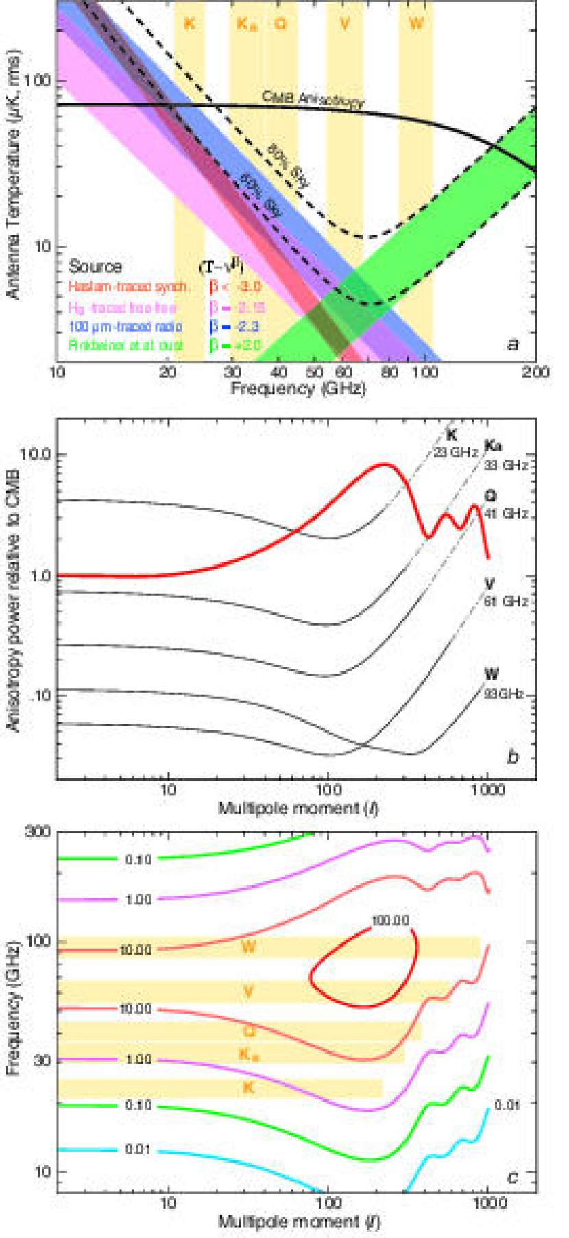
Figure 5: The frequency bands were chosen so that MAP observes the CMB anisotropy in a spectral region where the emission is most dominant over the competing galactic and extragalactic foreground emission. (a) Spectra are shown of CMB anisotropy (for a typical $\Lambda$CDM model) and estimates of galactic emission. A component traced by the Haslam spatial template (red) must be steep ($\beta<-3.0$) due to its lack of correlation with the COBE maps. (Note, however, that any template map of synchrotron emission will be frequency dependent, and hence the lack of correlation between Haslam and microwave maps is likely due to spatially variable spectral indices.) The free-free component (pink) estimate is from H$\alpha$ data (Haffner, et al., 2001; Gaustad et al., 2001), converted assuming $2\mu$K R^-1 at 53 GHz and a $-2.15$ spectral index. A component traced by 100 $\mu$m dust emission (blue) has a spectral index of $\beta\approx-2.3$ (Kogut et al., 1996b). This is likely to include the flat spectrum synchrotron emission that is relatively under-represented by 408 MHz Haslam template, but may be most of the synchrotron emission at microwave/millimeter wavelengths. Spinning dust emission components should be picked up in the H$\alpha$ (pink) and 100 $\mu$m (blue) estimates. The three component estimates, above, are partially redundant so they are added in quadrature to arrive at the estimate for the overall combined foreground spectra (dashed curves). The thermal dust emission model (green) of Finkbeiner, Davis & Schlegel (1999) is a fit to COBE data. The total galactic emission estimate is shown for cuts of the brightest microwave sky regions, leaving 60% and 80% of sky. (b) The spatial spectra are shown, in thermodynamic temperature, relative to a typical $\Lambda$CDM CMB model. 20% of the brightest galactic sky has been masked. The extragalactic source contribution of Toffolatti et al. (1998) is used with the assumption that sources down to 0.1 Jy have been removed. (c) The contour plot shows the ratio of CMB to foreground anisotropy power as a function of frequency and multipole moment. As can be seen, the MAP bands were chosen to be in the only region where the CMB anisotropy power is $>10\times$ to $>100\times$ that of the competing foregrounds. The MAP bands extend to an $l_{\rm{max}}$ such that the beam window function is 10%.

Microwave and other measurements show that at high galactic latitudes ($\left|b\right|>15^{\circ}$) CMB anisotropy dominates the galactic signals in the frequency range $\thicksim 30-150$ GHz (Tegmark et al., 2000; Tegmark & Efstathiou, 1996). However, the galactic foreground will need to be measured and removed from some of the MAP data. There are three conceptual approaches that can be used, individually or in combination, to evaluate and remove the galactic foreground.

The first approach is to use existing galactic maps at lower (radio) and higher (far-infrared) frequencies as foreground emission templates. These emission patterns can be scaled to the MAP frequencies and subtracted. Uncertainties in the external data and scaling errors due to position-dependent spectral index variations are the major weaknesses of this technique. There is no good microwave free-free emission template because there is no frequency where it clearly dominates the microwave emission. High-resolution, large-scale, maps of H$\alpha$ emission (Dennison, 2002; Haffner, et al., 2001; Gaustad et al., 2001) can serve as a template for the free-free emission, except in regions of high H$\alpha$ optical depth. The spatial distribution of synchrotron radiation has been mapped over the full sky with moderate sensitivity at 408 MHz (Haslam et al., 1981). Low frequency ($<10$ GHz) spectral studies of the synchrotron emission indicate that the intensities are reasonably described by a power-law with frequency $S\varpropto\nu^{\alpha}$ where $S(\nu)$ is the flux density, or $T\varpropto\nu^{\alpha-2}\equiv\nu^{\beta}$ where $T(\nu)$ is the antenna temperature and $\beta\thickapprox-2.7$, although substantial variations from this mean occur across the sky (Reich & Reich, 1988). There is also evidence, based on the local cosmic ray electronic energy spectrum, that the local synchrotron spectrum should steepen with frequency to $\beta\thickapprox-3.1$ at microwave frequencies (Bennett et al., 1992). However, this steepening effect competes against an effect that flattens the overall observed spectrum. The steep spectral index synchrotron components seen at low radio frequencies become weak relative to any existing flat spectral index components as one scales to the higher microwave frequencies. The synchrotron signal is complex because individual source components can have a range of spectral indices causing a synchrotron template map of the sky to be highly frequency-dependent. The dust distribution has been mapped over the full sky in several infrared bands, most notably by the COBE and IRAS missions. A full sky template is provided by Schlegel, Finkbeiner, & Davis (1998) and is extrapolated in frequency by Finkbeiner, Davis & Schlegel (1999).

The second approach is to form linear combinations of the multi-frequency MAP sky maps such that the galactic signals with specified spectra are canceled, leaving only a map of the CMB. The linear combinations of multi-frequency data make no assumptions about the foreground signal strength, but require knowledge of the spectra of the foregrounds. The dependence on constant spectral indices with frequency in this technique is less problematic than in the template technique, above, since the frequency range is smaller. The other advantage of this method is that it relies only on MAP data, so the systematic errors of other experiments do not enter. The major drawback to this technique is that it adds significant extra noise to the resulting reduced galactic emission CMB map.

The third approach is to determine the spatial and/or spectral properties of each of the galactic emission mechanisms by performing a fit to either the MAP data alone, or in combination with external data sets. Tegmark et al. (2000) is an example of combining spectral and spatial fitting. Various constraints can be used in such fits, as deemed appropriate. A drawback of this approach is the low signal-to-noise ratio of each of the galactic foreground components at high galactic latitude. This approach also adds noise to the resulting reduced galactic emission CMB map.

All three of these techniques were employed with some degree of success with the COBE data (Bennett et al., 1992). In the end, these techniques served to demonstrate that, independent of technique, a cut of the strongest regions of foreground emission was all that was needed for most cosmological analyses.

In addition to the galactic foregrounds, extragalactic point sources will contaminate the MAP anisotropy data. Estimates of the level of point source contamination expected at the MAP frequencies have been made based on extrapolations from measured counts at higher and lower frequencies (Park, Park & Ratra, 2002; Sokasian, Gawiser & Smoot, 2001; Refregier et al., 2000; Toffolatti et al., 1998). Direct 15 GHz source count measurements by Taylor et al. (2001) indicate that these extrapolated source counts underestimate the true counts by a factor of two. This is because, as in the case of galactic emission discussed above, flatter spectrum synchrotron components increasingly dominate over steeper spectrum components with increasing frequency. Microwave/millimeter wave observations preferentially sample flat spectrum sources. Techniques that remove galactic signal contamination, such as the ones described above, will also generally reduce extragalactic contamination. For both galactic and extragalactic contamination, the most affected MAP pixels should be masked and not used for cosmological purposes. After applying a point source and galactic signal minimization technique and masking the most contaminated pixels, the residual contribution must be accounted for as a systematic error.

Hot gas in clusters of galaxies will also contaminate the maps by shifting the spectrum of the primary anisotropy to create a Sunyaev-Zeldovich decrement in the MAP frequency bands. This is expected to be a small effect for MAP and masking a modest number of pixels at selected known cluster positions should be adequate.

Figures 5 illustrates how the MAP frequency bands were chosen to maximize the ratio of CMB-to-foreground anisotropy power. After applying data cuts for the most contaminated regions of sky, the methods discussed above are expected to substantially reduce the residual contamination.

5 INSTRUMENT DESIGN

5.1 Overview

The instrument consists of back-to-back Gregorian optics that feed sky signals from two directions into ten 4-channel polarization-sensitive receivers (“differencing assemblies”). The HEMT amplifier-based receivers cover 5 frequency bands centered from 23 to 93 GHz. Each pair of channels is a rapidly switched differential radiometer designed to cancel common-mode systematic errors. The signals are square-law detected, voltage-to-frequency digitized, and then down-linked.

5.2 Optical design

The details of the MAP optical design, including beam patterns and sidelobe levels, are discussed by Page et al. (2002). We provide an overview here.

Two sky signals, from directions separated in azimuth by $\sim 180^{\circ}$ and in total angle by $\sim 141^{\circ}$, are reflected via two nearly identical back-to-back primary reflectors towards two nearly identical secondary reflectors and into 20 feed horns, 10 in each optical path. The off-axis Gregorian design allows for a sufficient focal plane area, a compact configuration that fits in the Delta-rocket fairing envelope, two opposite facing focal planes in close proximity to one another, and an unobstructed beam with low sidelobes. The principal focus of each optical path is between its primary and its secondary.

The reflector surfaces are “shaped” (i.e. designed with deliberate departures from conic sections) to optimize performance. YRS Associates of Los Angeles, CA, carried out many of the relevant optical optimization calculations. Each primary is a (shaped) elliptical section of a paraboloid with a 1.4 m semi-minor axis and a 1.6 m semi-major axis. When viewed along the optical axis, the primary has a circular cross-section with a diameter of 1.4 m. The secondary reflectors are 0.9 m $\times$ 1.0 m. The reflectors are constructed of a thin carbon fiber shell over a Korex core, and are fixed-mounted onto a carbon-composite (XN-70 and M46-J) truss structure. The reflectors and their supporting truss structure were manufactured by Programmed Composites Incorporated. Use of the composite materials minimizes both mass and on-orbit cool-down shrinkage. The reflectors are fixed-mounted so as to be in focus when cool, so ambient pre-flight measurements are slightly out of focus. The reflectors have approximately 2.5 $\mu$m of vapor-deposited aluminum and 2.2 $\mu$m of vapor-deposited silicon oxide (SiO_x). The silicon oxide over the aluminum produces the required surface thermal properties (a solar absorptivity to thermal emissivity ratio of $\thickapprox 0.8$ with a thermal emissivity of $\thickapprox$0.5) while negligibly affecting the microwave signals. The microwave emissivity of coupon samples of the reflectors were measured in the lab to be that of bulk aluminum. The coatings were applied by Surface Optics Incorporated.

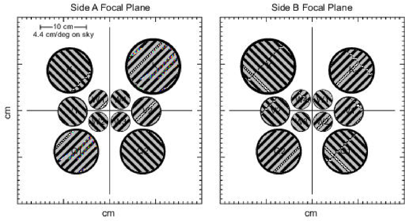
Figure 6: A view of the focal plane feed layout in the Focal Plane Assembly (FPA) as seen from the secondaries. The A-side is the $+y$ direction and the B-side is the $-y$ direction. The cross-hatch indicates the direction of the E-plane polarization for the axial OMT port. Each radiometer is named after the position of its feed pair, and the OMT ports to which it attaches. (We sometimes refer to feeds K and Ka as K1 and Ka1 despite the lack of a K2 and Ka2.) For example, for the radiometer V21, the last digit 1 corresponds to the axial OMT port while a last digit of 2 would indicate the radial OMT port. Radiometer V21 differences the polarizations shown by the hatching in this Figure. Radiometer V22 differences the opposite polarizations. With this convention, the meanings of all of the radiometer names can be immediately found from the above diagram.

The layout and polarization directions of the 10 feeds, covering five frequency bands, are shown in Fig. 6. The feed designs are driven by performance requirements (sidelobe response, beam symmetry, and emissivity), and by engineering considerations (thermal stress, packaging, and fabrication considerations), and by the need to assure close proximity of each feed tail to its differential partner.

The feeds are designed to illuminate the primary equivalently in all bands, thus the feed apertures approximately scale with wavelength. The smallest, highest frequency feeds are placed near the center of the focal plane where beam pattern aberrations are smallest. The HE₁₁ hybrid mode dominates the corrugated feed response, giving minimal sidelobes with high beam symmetry and low loss. The lowest frequency feeds are profiled to minimize their length, while the highest frequency feeds are extended beyond their nominal length so that all feeds are roughly of the same length. The feeds were specified and machined by Princeton University and designed by YRS Associates. They are discussed in greater detail by Barnes et al. (2002).

5.3 Radiometer design

The details of the radiometer design, including noise and 1/$f$ properties, are discussed by Jarosik et al. (2002). We provide an overview here.

MAP’s “Microwave System” consists of ten 4-channel differencing assemblies, each of which receives two orthogonally polarized signals from a pair of feeds. Each differencing assembly has both warm and cold amplifiers. The cold portion of each differencing assembly is mounted and passively-cooled in the Focal Plane Assembly (FPA) box; the warm portion is mounted in the Receiver Box (RXB).

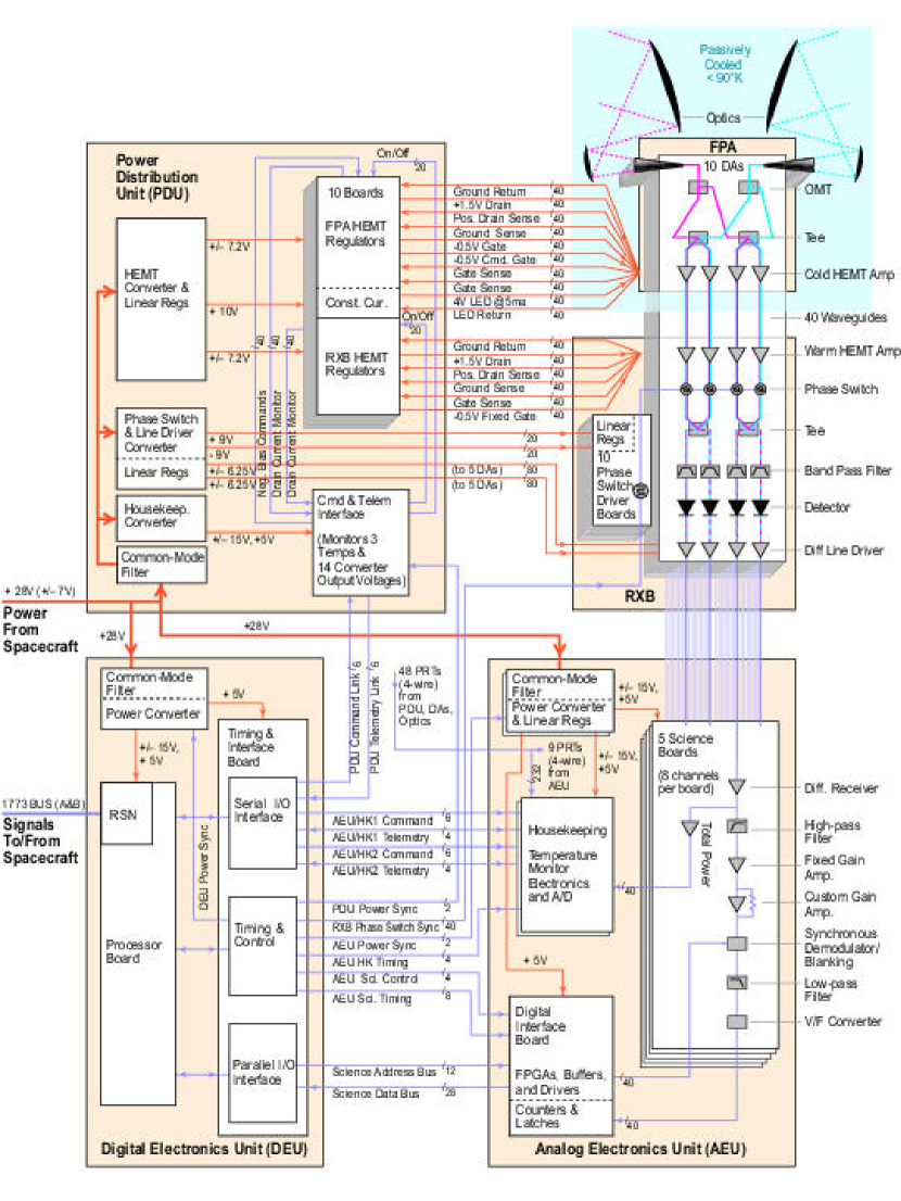
Figure 7: The instrument functional block diagram shows the interconnections between the instrument electronics and the differencing assemblies. Bold red lines are raw spacecraft power, thin red lines are instrument power, and thin blue lines are instrument signals.

As seen in Fig. 7, the signal from each feed passes through a low-loss orthomode transducer (OMT), which separates the signal into two orthogonal polarizations. The $A$-side signal is differenced against the orthogonally polarized signal from the opposite feed, $B^{\prime}$. This differencing is accomplished by first combining $A$ and $B^{\prime}$ in a hybrid Tee, amplifying the two combined outputs in two cold HEMT amplifiers, and sending the outputs to the RXB via waveguide. In the RXB the two signals are amplified in two warm HEMT amplifiers. Then one signal path is phase-switched (0^∘ or 180^∘ relative to the other) with a 2.5 kHz square-wave modulation. The two signals are combined back into $A$ and $B^{\prime}$ by another hybrid Tee, filtered, square-law detected, amplified by two line drivers and sent to the Analog Electronics Unit (AEU) for synchronous demodulation and digitization. The other pair of signals, $A^{\prime}$ and $B$, are differenced in the same manner. In MAP jargon, each of these pairs of signals comes from a “radiometer” and both pairs together from a “differencing assembly.” In all, there are 20 statistically independent signal “channels.”

The splitting, phase-switching, and subsequent combining of the signals enhances the instrument’s performance in two ways: (1) Since both signals to be differenced are amplified by both amplifier chains, gain fluctuations in either amplifier chain act identically on both signals, so common mode gain fluctuations cancel; and (2) The phase switches introduce a 180^∘ relative phase change between two signal paths, thereby interchanging which signal is fed into each square-law detector. Thus, low frequency (1/f) noise from the detector diodes is common mode and also cancels, further reducing susceptibility to systematic effects.

The first stage amplification operates at a stable low temperature to obtain the required sensitivity. HEMT amplifier noise decreases smoothly and only gradually with cooling; there are no sharp break-points. HEMT amplifiers exhibit larger intrinsic gain fluctuations when operated cold than when operated warm, so as many gain stages as possible operate warm, consistent with achieving the optimal system noise temperature.

The gate voltage of the first stage of the cold HEMT amplifiers is commandable in flight to allow amplifier performance to be optimized after the FPA has cooled to a steady-state temperature or as the device ages. Each pair of phase-matched chains (both the FPA and RXB portions) can be individually powered off in flight to prevent any failure modes (parasitic oscillations, excessive power dissipation, etc.) from interfering with the operation of other differencing chains.

The frequency bands (Jarosik et al., 2002; Page et al., 2002) were chosen to lie within commercial standards to allow the use of off-the-shelf components. The HEMT amplifiers (Pospieszalski, 2000; Pospieszalski et al., 1994; Pospieszalski, 1992) were custom-built for MAP by the National Radio Astronomy Observatory, based on custom designs by Marian Pospieszalski. The HEMT devices were manufactured by Loi Nguyen at Hughes Research Laboratories. The highest frequency band used unpassivated devices and the lower four frequency bands used passivated devices. The phase switches and bandpass filters were manufactured by Pacific Millimeter, the Tees and diode detectors by Millitech, the OMTs by Gamma-f, the thermal-break waveguide by Custom Microwave and Aerowave. Absorber materials, which are used to damp potential high-Q standing waves in the box cavities of the FPA and RXB, are from Emerson & Cummings. The differencing assemblies were assembled, tested, and characterized at Princeton University and the FPA and RXB were built up, aligned, tested, and characterized with their flight electronics at Goddard.

While noise properties were measured on the ground, the definitive noise values must be derived in flight since they are influenced by the specific temperature distribution within each radiometer.

The output of a square-law detector for an ideal differential radiometer is a voltage, $V$, per detector responsivity, $s$,

$$V/s = \left(\frac{A^{2}+B^{2}}{2}+n_{1}\right)g_{1}^{2}(t)$$

$$+\left(\frac{A^{2}+B^{2}}{2}+n_{2}\right)g_{2}^{2}(t)$$

$$\pm\frac{A^{2}-B^{2}}{2}g_{1}(t)g_{2}(t),$$

where $g$ and $n$ are the total gain and noise of each arm of a radiometer and $A$ and $B$ are the input voltages at the front-end of the radiometers. The first two terms are the total power signals. The $\pm$ on the third term alternates with the 2.5 kHz phase-switch rate, with the two arms of the radiometer always having opposite signs from one another. The difference between paired detector outputs for an ideal system,

$$V/s=(A^{2}-B^{2})g_{1}(t)g_{2}(t)=(T_{A}-T_{B})g_{1}(t)g_{2}(t)$$

is used to make the sky maps. See Jarosik et al. (2002) for a discussion of the effects of deviations from an ideal system.

5.4 Instrument electronics design

There are three instrument electronic components (see Fig. 7). The Power Distribution Unit (PDU) provides the instrument with its required regulated and filtered power signals. The Analog Electronics Unit (AEU) demodulates and filters the instrument detector outputs and converts them into digital signals. The Digital Electronics Unit (DEU), built into the same aluminum housing as the AEU, holds the instrument computer and provides the digital interface between the spacecraft and the PDU and AEU. The instrument electronics were built at Goddard.

The 5 science boards in the Analog Electronics Unit (AEU) take in the 40 post-detection signals from the RXB’s differencing assemblies through differential receivers. The 40 total power signals are split off and sent to the AEU housekeeping card for eventual telemetry to the ground. The total power signals are not used in making the sky maps due to their higher susceptibility to potential systematic effects, but they are useful signals for tracing the operation of the differencing assemblies and the experiment as a whole. After the total power signal is split off, the remaining signal is sent through a high-pass filter, a fixed gain amplifier, and then through another fixed-gain amplifier whose gain is set on the ground using precision resistors to accommodate the particular differencing assembly signal level. The signal is then demodulated synchronously at the 2.5 kHz phase-switch rate. A blanking period of 6 $\mu$sec (from 1 $\mu$sec before through 5 $\mu$sec after the switch event) is supplied to avoid systematic errors due to switching transients. The $\sim 40$ Hz bandwidth demodulated signal is then sent through a 2-pole Bessel low-pass filter with its 3 dB point at 100 Hz. Finally, the signal is sent through a voltage-to-frequency (V/F) converter, whose output is latched for read-out by the processor in the Digital Electronics Unit (DEU), before being losslessly compressed and telemetered to the ground. The AEU has a digital interface board and two power converter boards, which supply the requisite $\pm 15$ V, $\pm 12$ V, and $+5$ V to the other AEU boards.

The noise in each of the 40 AEU signal channels is limited to $<150$ nV Hz^-0.5 from 2.5 to 100 kHz to ensure that the AEU contributes $<1$% of the total radiometer noise. The AEU channel bandwidth is 100 kHz. The gain instability is $<5$ ppm for synchronous variations with the Observatory spin. This requires that the components be thermally stable to $<10$ mK at the Observatory spin rate. Random gain instabilities are limited to $<100$ ppm from 8 mHz (the spin frequency) to 50 Hz. The DC-coupled amplifier has random offset variations $<1$ mV rms from 8 mHz to 50 Hz to limit its contribution to the post-demodulation noise.

The AEU also contains two boards for handling voltage and high precision temperature sensing of the instrument. These monitors go well beyond the usual health and safety functions; they exist primarily to confirm voltage and thermal stability of the critical items in the instrument. Should variations be seen, these monitor signals can be used as tracers and diagnostics to characterize the effects on the science signals.

The DEU receives power from the spacecraft bus (fed through the PDU), applies a common-mode filter, and uses a DC-DC power converter to generate +5V and $\pm$15 V for internal use on its timing and interface board and on its processor board. The power converter is on one card while the Remote Services Node (RSN) (see §6.1) and timing boards are on opposite sides of a double-sided card.

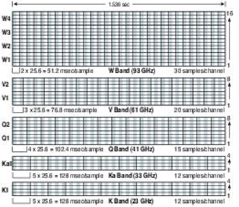
Figure 8: All 40 channels from the ten differencing assemblies are sampled in multiples of an underlying 25.6 ms period. The number of 25.6 ms periods that make up each sample is chosen with regard to the beamwidth of that channel to avoid smearing a source on the sky. Every 1.536 s the samples are collected and put into packets for later data down-link.

The DEU provides a 1 MHz ($\pm 0.005$% , 50% duty cycle) clock, derived from a 24 MHz crystal oscillator, to the V/F converter in the AEU. The DEU also supplies a 100 kHz clock to the power converters in the PDU and the AEU, a 2.5 kHz (50% duty cycle) clock to the RXB and AEU for phase switching, and a 5 kHz pulse to the AEU for blanking the science signal for 6 $\mu$sec during the 2.5 kHz switch transitions. The DEU also provides a 25.6 msec (64 cycles at 2.5 kHz = 39.0625 Hz) 1 $\mu$sec wide negative logic clock to the AEU for latching the 14-bit science data samples. All 40 channels are integrated in the AEU and sent to the DEU every 25.6 msec, as shown in Figure 8. The RF bias (total power) signals from the 40 AEU channels and 57 platinum resistance thermometer (PRT) temperature signals are passed from the AEU to the DEU every 23.04 seconds. All of these DEU clock signals are synchronous with the 24 MHz master clock. The DEU also sends voltage, current, and internal temperature data from the PDU, AEU, and DEU.

The 69R000 processor in the DEU communicates with the main computer (see §6.1) over a 1773 optical fiber bus. The DEU uses 12k (16-bit words) memory for generic RSN instruction code, 24k for DEU-specific code, and 10k for data storage.

The AEU and DEU are packaged together in an aluminum box enclosure with shielding between the AEU and DEU sections. The AEU/DEU and the PDU dissipate 90-95% of their power from their top radiators. They are qualified over a $-10$ to $+50$ C temperature range, but normally operate over a $0-40$ C range. The temperature variations of the boxes are designed to be limited to $<10$ mK peak-to-peak at the spin period. The 100 mil effective box wall thicknesses allow the electronics to survive the space radiation environment (see §6.6.2).

The PDU receives 21-35 V from the spacecraft, with spin-synchronous variations $<0.5$ V peak-to-peak, and provides all instrument power. Every HEMT gate and drain is regulated with a remote-sense feedback circuit. The PDU clamps the voltage between the gate and drain to be $<2.1$ V (at 10 $\mu$A) to prevent damage to the sensitive HEMT devices. The drain voltages are commandable in 8 steps ($\sim 70$ mV resolution) from 1.0 to 1.5 V, and the gates are commandable in 16 steps ($\sim 35$ mV resolution) from $-0.5$ V to 0 V. Voltage drifts are $\ll 10$ mV for the drain, and $\ll 5$ mV for the gates over the 0-40 C operating range.

The broadband noise requirements on the HEMT gate and drain supplies are: $<23f^{-0.45}$ $\mu$V Hz^-0.5 for 0.3 mHz - 1 Hz ($=885\;\mu$V Hz^-0.5 at 0.3 mHz); $<23\;\mu$V Hz^-0.5 for 1-50 Hz; and $<100$ nV Hz^-0.5 for 2.5 kHz and its harmonics to 50 kHz. These frequency ranges correspond to the precession frequency ($\sim 0.3$ mHz), the spin frequency ($\sim 7.57$ mHz), and the phase-switch frequency ($\sim 2.5$ kHz), respectively. Spin-synchronous rms variations are $<400$ nV.

The PDU supplies 4 V at 5 mA ($<5$ nA rms variation at the spin period) to two series LEDs on each cold HEMT amplifier. The LED light helps to stabilize the gain of the HEMT devices.

The PDU supplies $\pm 9$V ($<50$ mV ripple, $<20$ mV common mode noise) to the phase switch driver cards, which are mounted in the RXB, near the differencing assemblies. The PDU also supplies $\pm 6.25$ V to the line drivers in the RXB.

The PDU allows for on/off commands to remove power from any one or more of the 20 radiometers (phase-matched halves of the differencing assemblies). Should several radiometers be turned off such that the lack of power dissipation drives the PDU temperature out of its operational temperature range, a supplemental make-up heater can be commanded on to warm the PDU.

5.5 Instrument Calibration

The instrument is calibrated in-flight using observations of the CMB dipole and of Jupiter, as discussed in §7.1.

Despite the in-flight amplitude calibration (telemetry digital units per unit antenna temperature), it was necessary to provide provisional calibration on the ground to assess and characterize various aspects of the instrument to assure that all requirements would be met. For example, cryogenic microwave calibration targets (“x-cals”) were designed and built to provide a known temperature for each feed horn input for most ground tests. The x-cals, attached directly to each of the 20 feed apertures, were individually temperature-controlled to a specified temperature in the range of 15 K to 300 K, and provided for temperature read-out.

Observations of Jupiter and other celestial sources provide an in-flight pointing offset check relative to the star tracker pointing. The pointing directions of the feeds were measured on the ground using standard optical alignment techniques. Jupiter also serves as the source for beam pattern measurements in-flight. Beam patterns were measured in an indoor compact antenna range at the Goddard Space Flight Center and the far-sidelobes were measured between rooftops at Princeton University.

6 OBSERVATORY DESIGN

This section provides an overview of the MAP spacecraft systems. The physical layout of the Observatory is shown in Fig. 9 and the functional block diagram is shown in Fig. 10.

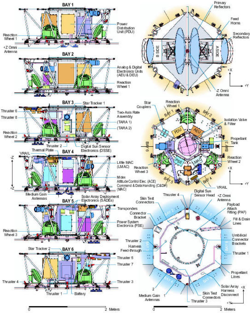
Figure 9: The physical lay-out of the Observatory is shown from various perspectives.

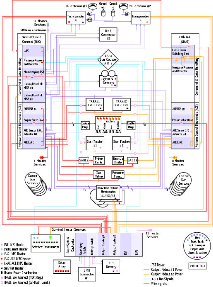
Figure 10: The functional block diagram of MAP shows the interconnections between the components.

6.1 Command and Data Handling

MAP implements a distributed architecture with a central Mongoose computer, which communicates via a 1773 (Spectran 171.2 $\mu$m 1300 nm polyamide) fiber optic bus to Remote Services Nodes (RSNs) located in the electronics boxes (see Figure 10). Each RSN provides a standardized interface to analog and digital electronics and uses common flight software. The RSN circuitry occupies half of one side of a printed circuit card; the remainder of the card space is used for application-specific circuitry. The fiber optics are interconnected using two (redundant) star couplers. Each is a pigtail coupler with a $16\times 16$ configuration in a 8.9 cm x 20 cm x 4.4 cm aluminum housing.

Attitude Control Electronics (ACE) and Command and Data Handling (C&DH) functions are housed in the Midex ACE and C&DH (MAC) box, which contains 9 boards: (1) A Mongoose V R3000 32-bit rad-hard RISC processor board includes 4 MB of EEPROM memory and 320 MB of DRAM memory (of which 224 MB is for the solid state data “recorder”, 32 MB is for code, and 64 MB is for check-bytes), with 4 Mbps serial outputs to the transponder interface boards and redundant 1773 interfaces; (2,3) Two Low Voltage Power Converter (LVPC) boards (see §6.4); (4,5) Two up- and down-link transponder boards, which are both always active (see §6.3); (6) A housekeeping board, which monitors 6 deployment potentiometers (see §6.5), 9 status indicators, 46 temperature channels, and 2 voltages, in addition to one spare word, for a total of 64 input signals; (7) An ACE RSN and sensor electronics I/O board, which reads the digital and coarse sun sensors, and reads and commands the reaction wheels (see 6.2); (8) An ACE sensor I/O board that queries and/or reads information from the inertial reference unit (gyro), digital and analog Sun sensors, reaction wheels, separation switches (see 6.2), and sends a timing pulse to the star trackers and monitors thermistors and solar array potentiometers; and (9) A propulsion engine valve drive (EVD) electronics board that controls the 8 thrusters (see §6.2).

Selected redundancy is provided by a “Little MAC”, or LMAC box. The LMAC box houses a total of six boards. Four boards hold the redundant attitude control electronics (an LVPC board, a EVD electronics board, a sensor I/O board, and an RSN board). The two remaining boards are a redundant Mongoose processor board, and a LVPC board with power switching circuitry that controls the redundancy between the MAC and the LMAC functions. Only one Mongoose processor (MAC or LMAC) is on and in control at any one time. Shortly after launch the LMAC ACE takes primary control, with the MAC ACE powered on as a “hot” back-up. The active Mongoose processor board sends an “I’m OK” signal to the LMAC ACE. If the LMAC ACE fails to get the “I’m OK” signal, then it places the Observatory into safe-hold. That is, the ACE RSN acts as an attitude control safehold processor. If the housekeeping RSN fails, the LMAC ACE is powered on by ground command. Only a single uplink path can be active, selected by ground command.

6.1.1 Data Sampling and Rates

The MAC Mongoose processor gathers the Observatory science and engineering data and arranges them in packets for down-link. The instrument’s compressed science data comprises 53% of the total telemetry volume.

As shown in Fig. 8, during a 1.536 sec period the instrument collects 30 samples in each of 16 W-band (93 GHz) channels, 20 samples in each of 8 V-band (61 GHz) channels, 15 samples in each of 8 Q-band (41 GHz) channels, and 12 samples in each of 4 Ka-band (33 GHz) and 4 K-band (23 GHz) channels. In this way the bands with smaller beams are sampled more often. With 856 samples all together at 16 bits per sample in 1.536 sec, there is a total instrument science data rate of 8917 bits s^-1. The instrument science data is put into two packets, with all of the W-band data in one packet and all other data in a second packet. The second packet is assigned some additional filler to make the two packet lengths identical. Each packet also has 125 bits s^-1of “packaging” overhead. The adjusted total raw instrument data rate is 9042 bits s^-1. These data flow from the DEU to the MAC.

The Mongoose V processor losslessly compresses this data on-the-fly by a factor of $\approx 2.5$ using the Yeh-Rice algorithm, and then records 3617 bits s^-1of science data. An additional 500 bits s^-1of instrument house-keeping data and 2750 bits s^-1of spacecraft data are recorded, for a total of 6867 bits s^-1. The $\approx 0.6$ Gbits of data per day are down-linked daily. Of the overall down-link rate of 666666 bits s^-1, 32000 bits s^-1are dedicated to real-time telemetry, and 563167 bits s^-1are allocated to the playback of the stored data, which takes 17.6 min. The bit rate is commandable and may be adjusted in flight depending on the link margins actually achieved.

6.1.2 Timing control

The Mongoose board in the MAC/LMAC maintains time with a 32-bit second counter and a 22-bit microsecond counter. There is also a watchdog timer and a 16-bit external timer. The clock is available to components on the bus with a relative accuracy of 1 ms. Data are time-tagged so that a relative accuracy of 1.7 ms can be achieved between the star tracker(s), gyro, and the instrument. The Observatory time is correlated to ground time to within 1 s.

6.2 Attitude and Reaction Control

The attitude control system (ACS) takes over control of the orientation of the Observatory after its release from the Delta vehicle’s third stage. From the post-separation $3\sigma$ initial conditions ($\pm 2^{\circ}$ s^-1 $x$- and $y$-axis tip-off rates, and $\pm 2$ rpm $z$-axis de-spin rate), MAP is designed to achieve a power-positive attitude (solar array normal vector within 25^∘ of the Sun direction) within 37 min using only its wheels for up to 2$\sigma$ tip-off rates.

The attitude control and reaction control (propulsion) systems bring MAP through the Earth-Sun phasing loops (see Fig. 3) such that the thrust is within $\pm 5^{\circ}$ of the desired velocity vector with 1^∘ maneuver accuracy. After the lunar-swingby, MAP cruises, with only slight trajectory-correction mid-course maneuvers, into an orbit about L₂. Once there, the ACS provides a combined spin and precession such that the Observatory spin ($z$) axis remains at $22.5^{\circ}\pm 0.25^{\circ}$ from the Sun vector for all science observations. This is referred to as “Observing Mode.” For all maneuvers that interrupt Observing Mode (after the mid-course correction on the way to L₂, and for station-keeping maneuvers at L₂) the spin ($z$) axis must always remain at $19\mbox{${}^{\circ}$}\pm 5\mbox{${}^{\circ}$}$ relative to the anti-Sun vector to prevent significant thermal changes. The spin rate must be an order of magnitude higher than the precession rate and the instrument boresight scan rate must be $2.59\mbox{${}^{\circ}$}$ s^-1 to $2.66\mbox{${}^{\circ}$}$ s^-1. The $2.784\mbox{${}^{\circ}$}$ s^-1 ($0.464$ rpm) spin and the $0.100\mbox{${}^{\circ}$}$ s^-1 (0.017 rpm, 1 rev hr^-1) precession rates are in opposite directions and are controlled to within 6%. The ACS must also manage momentum and provide an autonomous safe-hold. Momentum management occurs throughout the mission, with each momentum unload leaving $\mbox{${}_{<}\atop{}^{\sim}$}0.3$ Nms per axis.

The instrument pointing knowledge requirement of 1.3 arcmin ($1\sigma$) is sufficient for the aspect reconstruction needed to place the instrument observations on the sky. Of this, 0.9 arcmin (a root-sum-square for 3 axes) is allocated to the attitude control system.

The radius of the Lissajous orbit about L₂ (see Fig. 3) must be $\mbox{${}_{>}\atop{}^{\sim}$}0.5\mbox{${}^{\circ}$}$ (between the Sun-Earth vector and the Earth-MAP vector) to avoid eclipses, and $<10.5\mbox{${}^{\circ}$}$ to maintain the antenna angles necessary for a sufficient communication link margin.

The attitude and reaction control systems include attitude control electronics (ACE boards, in both the MAC and LMAC boxes), 3 reaction wheels, 2 digital Sun sensors, 6 prime plus 6 redundant coarse Sun sensors, 1 gyro (mechanical dynamically-tuned, consisting of 2 TARAs = Two-Axis Rate Assemblies), and 2 star trackers (one prime and one redundant). The propulsion system consists of two engine valve drive cards (one in the MAC box and a redundant card in the LMAC box), a hydrazine propulsion tank with stainless steel lines to 8 thrusters (2 roll, 2 pitch, 2 yaw, and 2 backups), with an isolation valve and filter. (The fuel filter is, appropriately enough, a hand-me-down from the COBE mission.)

The Lockheed-Martin model AST 201 star trackers are oriented in opposing directions on the $y$-axis. They are supplied with a 1773 interface, track at a rate of 3^∘ s^-1, and provide quaternions with an accuracy of 2.3 arcsec in pitch and yaw, and 21 arcsec (peak) in roll.

The TARAs are provided by Kearfott. One TARA senses $x$ and $z$ rates and the other senses $y$ and $z$ rates over a 12^∘ s^-1 range. The TARAs provide a digital pulse train (as well as analog housekeeping) with 1 arcsecond per pulse. The linear range is $\pm 5^{\circ}$ s^-1 with an angle random walk of $<0.03^{\circ}$ hr^-1.

The digital Sun sensors are provided by Adcole. The two digital Sun sensors each provide a field-of-view that extends $\pm 32^{\circ}$ from its boresight, and they are positioned to provide a slight field-of-view overlap. The output has two serial digital words and analog housekeeping. The resolution is $0.004^{\circ}$ (0.24 arc min) and the accuracy is 0.017^∘. The 12 coarse Sun sensors (6 primary and 6 redundant) are also provided by Adcole. They are mounted at the outer edge of each solar panel and are positioned with boresight angles pointed alternately 36.9^∘ towards the instrument (bays 2, 4, 6) and 36.9^∘ towards the Sun (bays 1,3 5) with respect to the plane of the solar arrays. Their fields of view extend $\pm 85^{\circ}$ from each of the boresights. They provide an attitude accuracy of better than 3^∘ when uncontaminated by Earth albedo effects. Their output is a photoelectric current.

The Ithaco Type-E reaction wheel assemblies have a maximum torque of $\pm 0.35$ Nm, but the MAP ACE limits this to $\pm 0.177$ Nm ($<125$ Watts per wheel, $<5.3$ amps per wheel) to control power use, especially for the high wheel rates that potentially could be encountered during initial acquisition. MAP’s maximum momentum storage is $\pm 75$ Nms. The wheels take an analog torque input and provide a tachometer output.

The propulsion tank, made by PSI, was a prototype spare unit from the TOMS-EP Program, which kindly provided it for use on MAP . It has a titanium exterior, which is only 0.076 cm thick at its thinnest point, with an interior elastomeric diaphragm to provide positive expulsion of the hydrazine fuel. The tank is roughly 56 cm in diameter, has a mass of 6.6 kg, and holds 72 kg of fuel.

The eight 4.45 N thrusters are provided by Primex. Each thruster has a catalyst bed heater that must be given at least 0.5 hr to heat up to at least 125 C before a thruster is fired. The fuel must be maintained between 10 C and 50 C in the lines, tank, and other propulsion system components, without the use of any actively controlled heaters. A zone heating system was developed to accomplish this relatively uniform heating of the low thermal conductivity (stainless steel) fuel lines that run throughout the Observatory. The lines, which are wrapped in a complex manner that includes heaters and thermostats, are divided into thermal zones. The zones were balanced relative to one another during Observatory thermal balance/thermal vacuum testing. In flight, zone heaters can be switched on and off, by ground command, to provide re-balancing, but this is not expected and, if needed, would be far less frequent switching than would be the case with an autonomously active thermal control system. In this way the Observatory thermal and electrical transitions will be minimal.

A plume analysis was performed to determine the amount of hydrazine byproduct contamination that would be deposited in key locations, such as on the optical surfaces. These analyses take into account the position and angles of the eight thrusters. The final thruster placement incorporated the plume analysis results so that byproduct contamination levels are acceptably low.

The ACS provides six operational modes, described below.

Sun Acquisition mode uses reaction wheels to orient the spacecraft along the solar vector following the Delta rocket’s yo-yo despin (to $<2$ rpm) and release of the Observatory from the third stage. This must be accomplished $<37$ mins after separation due to battery power limitations. The body momentum is transferred to the reaction wheels until the angular rate is sufficiently reduced, and then position errors from the coarse Sun sensors and rate errors from the inertial reference unit are nulled.

Inertial mode orients and holds the Observatory at a fixed angle relative to the Sun vector in an inertially fixed power-positive orientation, and provides a means for slewing the Observatory between two different inertially fixed orientations. Reaction wheels generate the motion and the IRU (gyro) provides sensing. Inertial mode can be thought of as a “staging” mode between Observing, Delta-H, or Delta-V modes. Information from the digital Sun sensor and star tracker are used in a Kalman filter to update the gyro bias and quaternion error estimates and these data are used by the controller.

Observing mode moves the Observatory in a compound spin (composed of a spin about the $z$-axis combined with a precession of the $z$-axis about the anti-Sun vector) that satisfies the scientific requirements for sky scanning. The total reaction wheel momentum is canceled by the prescribed body momentum. The Kalman filter is used in the same manner as in the Inertial mode, described above.

Delta-H mode is used to change the Observatory’s angular momentum. It is used following the yo-yo de-spin from the Delta rocket’s third stage for $>2\sigma$ tip-off rates, and to reduce wheel momentum that accumulates later in the mission. Thrusters can be used as a back-up in the unexpected event that the Observatory has more momentum than can be handled by the reaction wheels. A pulse width modulator is used to convert rate controller information to thruster firing commands. The reaction wheel tachometers are used along with the IRU to estimate the total system momentum.

Delta-V mode is used to change the Observatory’s velocity. It is used in the initial phasing loop burns and for station-keeping near L₂. The controller must account not only for the desired combination of thrusters and degree of thruster firings, but must also assure that position and rate errors (which may arise from center-of-mass offsets, thruster misalignments, or plume impingement) are maintained within allowable limits.

Safe-hold mode slews the Observatory to an inertially fixed power-positive orientation. Reaction wheels are used to move the Observatory according to coarse Sun sensor information. Safe-hold functions are similar to Sun Acquisition functions, except that Safe-hold mode can use only the coarse Sun sensors, not the IRU. The IRU mode allows control with higher system momentum.

6.3 RF Communications

MAP carries identical prime and redundant transponders, each capable of communications on both the NASA Space Network (SN) and Ground Network (GN). Each S-band (2 GHz) transponder has an output power of $\geq 5\$W. The prime and redundant transponders are controlled by RSN boards in the MAC and LMAC boxes.

Two omnidirectional (“omni”) antennas, each with 0 dBi gain over $\pm 80^{\circ}$ from the boresight, combine to provide nearly full spherical coverage for use should the Observatory attitude be out of control. The omni antennas (like those on the XTE, TRMM, and TRACE missions) are crossed bow-tie dipoles, built in-house at Goddard. Because one of MAP ’s omni antennas will never be in sunlight during nominal science operations, the omni antenna and its Gore coaxial cable were tested at Goddard for $-200^{\circ}$ C operation.

MAP carries two medium gain antennas for high speed data transmission to Earth. The medium gain antennas, designed, built and tested at Goddard, use a circular PC-board pattern to provide $\geq 5.5$ dBi gain over $\pm 35^{\circ}$ from the boresight. They have been designed and tested for $\pm 100^{\circ}$ C, while nominally in 100% sunlight during most of the mission. The antennas have a Goretex thermal protective cover.

The RF communications scheme is shown as part of Fig. 10. Each of the two transponders receives from its own medium gain and both omni antennas at all times. Microwave switches allow each transponder to transmit to both of the omni antennas or, alternately, to its medium gain antenna.

6.4 Power System

The power system provides at least 430 Watts for 30 min to assure that safehold can be reached, and 430 Watts of average orbital power at the end of 27 months for the L₂ orbit at $22.5\mbox{${}^{\circ}$}\pm 0.25\mbox{${}^{\circ}$}$. The system is designed such that the battery depth of discharge is never worse than 60%.

The power system consists of six GaAs/Ge solar array panels, a NiH₂ battery, a Power Supply Electronics (PSE) box, and Low Voltage Power Converter (LVPC) cards located in other electronics boxes.

The solar panels are supplied by Tecstar, Inc. To keep the instrument passively cool, MAP requires that the backs of the solar panels be covered with thermal blankets. In this unusual configuration, steps must be taken to keep the panels from overheating. Thus, much of the Sun-side surface area that is not covered by solar cells is covered by second surface mirrors (optical surface reflectors) that allow the panels to reject heat by reflecting sunlight rather than absorbing it. The solar panels are specified to supply $>678$ Watts at $>34.6$ Volts at the beginning of life, and $>502$ Watts at $>31.5$ Volts after 27 months of flight, both at 86 C. Each of the 6 solar panels includes 14 strings of 48 (4.99 cm x 5.65 cm) GaAs/Ge cells each, with a total solar cell area of 5187 cm² for each of the 6 panels, with a solar absorptance of $>0.87$ averaged over the solar spectrum.

The nickel hydrogen (NiH₂) battery is a 23 amp-hr common pressure vessel design that consists of 11 modules, each of which contains two cells that share common electrolyte and hydrogen gas. It is supplied by Eagle Picher Technology of Joplin, MO. The battery is capable of supplying about 35 V when freshly charged. (The Observatory is nominally expected to operate at about 31.5 V.) The solar array is deployed after Observatory separation from the launch vehicle, allowing the battery to recharge once the power system is power-positive on the Sun.

The PSE and LVPCs were designed and built by Goddard. The PSE’s LVPC supplies switched and unswitched secondary power ($\pm 15$V, $+5$V), and it provides unregulated switched primary power to loads in the subsystem in which it is located.

In case of emergency, the on-board computer will autonomously begin taking action, including shedding loads. The power system uses a pre-programmed relationship between the battery temperature and voltage (a “V/T curve”) in an active control loop. When the battery reaches a 90% state-of-charge (SOC) and the bus voltage drops below 30 V, a warning is issued by the Observatory and the PSE is set to its normal operating V/T relationship. At an 80% state-of-charge and a bus drop to 27 V, the instrument, catalyst bed heaters, makeup heaters and battery operational heater are all autonomously turned off and the Observatory goes into safe-hold. At 60% state-of-charge and $<26$ V the second star tracker is turned off. At 50% state-of-charge and $<25$ V the PDU make-up heater, RXB operational heater, and solar array dampers heaters are all turned off. Although all components have been tested to operate properly at as low as 21 V, this condition can not be supported in steady-state for more than a couple of hours. This is long enough only for emergency procedures to take control and attempt to fix a problem.

6.5 Solar Array Deployment System

Web thermal blanket segments run from center-line to center-line on the anti-Sun side of the six solar array panels. The panels are folded for launch to $5\mbox{${}^{\circ}$}$ from the $z$-axis, with the blankets tucked gently inside. The panels are held in place by a Kevlar rope that runs around the external circumference of the spacecraft, in V-groove brackets, and is tensioned to almost 1800 N against a spring-loaded hot knife. The knife, a circuit board with high ohmic loss traces, is activated with a voltage that is applied based upon an on-board timing sequence keyed to separation of MAP from the launch vehicle. Redundant thermal knives are on opposite sides (bays 3 and 6) of the Observatory. An automated sequence fires one knife first, and then the second knife is energized after a brief time delay.

Each solar array panel is mounted with springs and dampers. Once the tensioned Kevlar cable is cut it departs the Observatory at high speed. Then the panels and web blankets gently unfold together (in $\sim 15$ s) into the $z=0$ plane.

6.6 Mitigation of Space Environment Risks

6.6.1 Charging

Spacecraft charging can be considered in two broad categories: surface charging and internal charging.

The various external surfaces, whether dielectric or conductive, will be exposed to a current of charged particles. If various surfaces are not reasonably conductive ($<10^{9}\Omega$ square^-1) and tied to the Observatory ground then differential charging will occur. Differential charging leads to potential differences that can discharge either in sudden and large sparking events, or in a series of smaller sparks. In either case these discharges can cause severe damage.

For space missions in low Earth orbit the local plasma can be effective in safely shorting out potential charge build-ups. Components in sunlight also have the advantage of discharge via the photoelectric effect. MAP does not have the benefit of a local, high-density, plasma, and much of the Observatory is in constant shadow. Thus, with only a few well-considered exceptions, MAP was built with external surfaces that are in reasonable conductive contact with one another. Conductive surfaces used on MAP include indium-tin-oxide coatings on teflon, silver teflon, and paint, and carbon-loaded (“black”) kapton.

The Observatory is also exposed to a current of higher energy particles that penetrate the skin layer materials and can deposit charge anywhere in the Observatory, not just on its surface. Only radiation shielding in the form of mass can stop the high energy particles, and mass is always a precious resource for a space mission. MAP used a complex set of implementation criteria to protect against internal charging. This protection can not be absolute: there is a power spectrum of incoming radiation, the current amplitudes as a function of location are uncertain, and the stopping power of shielding is statistical. In general, the MAP interior surfaces are grounded where possible, and a minimal amount of external shielding metal (either boxes, plates, or added lead shielding) is used to reduce the size of the charging currents. All susceptible circuits were shielded with an equivalent stopping power of 0.16 cm of aluminum. For example, 0.2 mm of lead foil was wrapped around all the bias and control lines of the HEMT amplifiers to augment the existing harness shielding.

6.6.2 Radiation

Extended exposure of the Observatory to a very high energy radiation environment can cause components to degrade with total dose. For MAP the ambient environment at L₂ is not severe, but the passages through the Earth belts during the early phasing loops can give a significant dose in a short time. The predicted total ionizing dose (TID) of radiation exposure at the center of a 2.54 mm thick aluminum shell, in MAP ’s trajectory over the course of 27 months, is $\approx 13.5$ krad. For safety, and to cover model uncertainties, a factor of two margin was imposed on this prediction, so MAP was designed to withstand 27 krad TID. Ray tracing of the actual MAP geometry shows that most electronics boards are exposed to about $5-10$ krad.

MAP is also designed to a requirement to survive single event upsets at a level of $35$ MeV cm² mg^-1 linear energy transfer (LET; the energy left by an energetic particle), without degraded performance.

6.6.3 Micrometeoroids

Any object of substantial size in space will be subject to bombardment by micrometeoroids. For MAP micrometeoroids may puncture the MLI webbing between the solar shields (allowing a limited amount of sunlight to illuminate the optics and diffract into the feeds) and impact the optics (increasing their emissivity). Holes in the Sun shield would transmit solar energy, while holes in the reflectors would emit as blackbody sources at 70 K, the approximate temperature of a reflector. For the isotropic distribution of micrometeoroids believed to be representative of L₂, a solar leak through punctured webbing will not produce a net signal larger than 0.5 $\mu$K at 93 GHz, even in the absence of the diffraction shield. For the duration of the mission, the offset from random micrometeoroids hitting the primaries is expected to be smaller than $0.5~{}\mu$K at the 95% confidence level if the holes are the size of the micrometeoroids. If the holes are five times larger than the micrometeoroids that produced them, which is not out of the question, the offset will be negligible: $<140~{}\mu$K in 95% of the cases. Damage to the reflectors is dominated by rare encounters with 100 $\mu$m size particles. See Page et al. (2002) for a more detailed discussion of the effects of micrometeoroids on the MAP optics.

6.7 Launch and Trajectory

A Delta 7425-10 expendable launch vehicle places MAP into a $28.7\mbox{${}^{\circ}$}$ inclination near-circular orbit from the NASA Kennedy Space Center Eastern Test Range. The Delta third stage fires, de-spins, and then separates from MAP , placing MAP into a highly eccentric orbit reaching nearly to the lunar distance. The specific energy (energy per unit mass) of the launch was fixed at C${}_{3}=-2.6$ km² s^-2 to place a maximal amount of mass into orbit. The Delta vehicle uses four graphite epoxy motors (GEMs), a STAR-48 third stage, and a 3.048 m composite fairing. The absolute value of the launch vehicle velocity error is $<11.6$ m s^-1($3\sigma$). MAP is attached to the vehicle with a 3712C payload adapter fitting. During the launch the payload experiences accelerations of 11.3 g along the thrust axis and 3.5 g laterally.

Three general options were examined for a trajectory to L₂: a direct transfer, a lunar-assisted direct transfer, and a lunar-assisted transfer with Earth-Moon “phasing loops” (i.e., highly eccentric Earth orbits). The final option was selected based on its fuel efficiency, and based on its tolerance for initial problems since there are no critically important maneuvers that need to be executed for at least 2 or 3 days after launch. The lunar gravity-assist requires an orbit apogee of approximately the lunar orbit distance of $\sim$400,000 km with a line of apsides oriented such that MAP passes just behind the Moon at apogee (a “trailing swingby”). The most efficient gravity-assist occurs when the Moon approaches the anti-Sun direction, near full Moon. Phasing loops are used to avoid the narrow launch window otherwise imposed by the lunar-assist and to allow time to correct launch vehicle errors and gain spacecraft operational experience before critical maneuvers must take place. Two through five loop scenarios are possible, although only 3 and 5 loop cases are accepted by MAP since they have the least risk. Mid-course correction(s) apply final corrections following the lunar swingby and before the Observatory attains a Lissajous orbit about the L₂ point. Fig. 3 shows a sample MAP trajectory to L₂. The Goddard Space Flight Center has done relevant previous trajectories for the L₁ missions WIND, SOHO, and ACE.

The natural growth of trajectory errors in orbit about L₂ will result in the need to execute small station-keeping trim maneuvers approximately every three months. Momentum unloading is accomplished at the same times to minimize thermal disruptions to the Observatory.

6.8 Ground Operations

Data from the satellite is transferred through NASA’s Deep Space Network (DSN), to a combined Science and Mission Operations Center (SMOC), located at the Goddard Space Flight Center. Very little in the way of science operations activities are required for the MAP mission due to the survey nature of the mission and the desire to minimize all disturbances to the Observatory. The SMOC monitors the basic health and safety of the Observatory, sends all commands, and transfers level-0 data (data that passes parity checks and is in time-order) to the Office of the MAP Experiment’s General Archive (OMEGA).

Two mission design features were implemented to assist the operations team. First, there is on-board fault protection. Software in the attitude control system can detect a fault, switch in redundant hardware, and switch to a simple safe-hold mode to buy time for personnel on the ground to determine exactly what happened and to correct the problem before returning MAP to Observing mode. Software in the power system can detect a low voltage or low battery state-of-charge and react by restoring proper settings and shedding loads. Second, the system supplies the ground with error and status measurements and telemetry to inform the ground that something has gone wrong or is out of limits. Generally, the spacecraft informs the ground that something is threatening the spacecraft health and safety.

7 DATA ANALYSIS

The MAP Science Team must: check the data to assure that all operations appear to be proper; assure that the instrument is operating optimally; check the data, in great detail, for evidence of systematic errors; attempt to correct any such errors; and calibrate the data and transform it from time-ordered to a map of the sky according to Wright, Hinshaw & Bennett (1996a). The idea is to guess a map of the sky, and then improve the guess iteratively using the differential data. These iterations can include polarization maps and a calibration solution. The map data must also be carefully checked for systematic errors. The heart of the data processing task is to place quantitative upper limits on potential systematic measurement errors.

7.1 Systematic Error Analysis

The raw differential data may be modeled in the form

$$d(t) = g(t)\left[\Delta T(t)+s(t)+o(t)\right]+n(t)$$

$$= \left[g_{0}(t)+g_{1}(t)\right]\left[\Delta T(t)+s(t)+o_{0}(t)+o_{1}(t)\right]+n(t)$$

$$= g_{0}(t)\Delta T(t)+g_{0}(t)s(t)+g_{0}(t)o_{0}(t)$$

$$+\,g_{0}(t)o_{1}(t)+g_{1}(t)o_{0}(t)+n(t)+\cdots$$

where $d(t)$ is the raw time-stream in uncalibrated digital units, $g(t)$ is the true radiometer gain, in du mK^-1, $\Delta T(t)$ is the true differential sky temperature, in mK, $s(t)$ is the signal due to uncorrected differential signals, in mK, that act on the instrument sidelobes, $o(t)$ is the instrument offset, in mK, which is the signal that would be measured with a nulled input signal, and $n(t)$ is the instrument noise produced either by the amplifiers, or by miscellaneous pick-up after signal amplification. It is useful to expand the gain and offset in a form of perturbation series, where $g_{0}(t)$ and $o_{0}(t)$ are the dominant, slowly varying terms and $g_{1}(t)$ and $o_{1}(t)$ are the smaller, more rapidly fluctuating terms. Terms of order $g_{1}o_{1}$ are dropped in the last line of the above expression.

As part of the data processing, known modulation due to the CMB dipole is used to fit for an instrument gain and baseline (see §7.2). Noise levels are such that reasonable sensitivity (to better than 1%) to each term is achieved with about an hour of data. Since this matches the spacecraft precession period, it marks a characteristic time scale for the above perturbation expansion. Gain and offset changes can be tracked on time scales greater than one hour directly from the sky data, while other means must be employed to track changes on shorter time scales, particularly at the spin period since these changes can most closely mimic a true sky signal.

In processing the data, smooth fits to the gain and baseline solutions are generated, and are denoted the recovered gain and baseline, $g^{\prime}(t)$ and $b^{\prime}(t)$, respectively. The recovered differential temperature is then

$$\Delta T^{\prime}(t) = \left[d(t)-b^{\prime}(t)\right]/g^{\prime}(t)$$

$$= \left[g_{0}\Delta T+g_{0}o_{0}+g_{0}o_{1}+g_{0}s\right.$$

$$\left.+\,g_{1}o_{0}+n-b^{\prime}\right]/g^{\prime}+\cdots$$

$$= (g_{0}/g^{\prime})\Delta T+\left[(g_{0}/g^{\prime})o_{0}-b^{\prime}/g^{\prime}\right]$$

$$+\,(g_{0}/g^{\prime})o_{1}+(g_{0}/g^{\prime})s+(g_{1}/g^{\prime})o_{0}+n/g^{\prime}+\cdots$$

where the explicit time dependence in each term is dropped. Note that the true baseline and the true offset are related by the gain, $b(t)=g(t)o(t)$.

Systematic errors in the final sky maps can originate from a variety of sources that can be classified according to which term they contribute to in the above expansion. These include:

• Calibration errors. These calibration errors, from any source, contribute to making $(g_{0}/g^{\prime})$ differ from unity and to making $(g_{0}/g^{\prime})o_{0}-b^{\prime}/g^{\prime}$ differ from zero. (see §7.2)

• External emission sources. These include errors due to spin-synchronous modulations of the emission from the Sun, Earth, Moon, and Galaxy acting on the instrument sidelobes, or due to the local Doppler effect producing an induced signal. These contribute to $(g_{0}/g^{\prime})s$ (see §7.3).

• Internal emission sources. These errors are due to spin-synchronous temperature variations acting on components with fixed emissivities. These effects contribute to $(g_{0}/g^{\prime})o_{1}$ by varying the instrument offset (see §4.1).

• Multiplicative electronics sources. These errors are due to spin synchronous gain variations acting on a fixed radiometric offset. These effects contribute to $(g_{1}/g^{\prime})o_{0}$ (see §5.4).

• Additive electronics sources. These errors are due to miscellaneous spin-synchronous electronics errors, such as instrument channel-channel cross-talk. These contribute to $n(t)$, which needn’t be random, or white (see §5.3).

• Striping. These effects can be introduced by correlations in the instrument noise, due either to 1/f effects or to post-detection filtering, or due to the effects of scan smearing and intrinsic beam ellipticity.

• Map-making errors. These errors are due to poor convergence or striping introduced by the map-making algorithm, possibly in concert with calibration errors. Also errors due to pointing uncertainty.

• Beam mapping errors. These are errors in the determination of the main beam window function that directly contribute to errors in the recovered power spectrum.

7.2 Calibration Analysis

For a sufficiently short period of time the instrument gain and baseline can be approximated as constant,

$$d(t)\approx g_{n}\Delta T(t)+b_{n}$$ (1)

where $g_{n}$ and $b_{n}$ are the gain and baseline during the $n^{\rm th}$ calibration period. Since the sky signal $\Delta T$ is dominated by the (known) CMB dipole $\Delta T_{d}$ (including the time-dependent modulation from MAP ’s velocity relative to the Sun), the raw data for a gain and a baseline can be fit by minimizing

$$\chi^{2}=\sum_{i}\frac{\left(d(t_{i})-(g_{n}\Delta T_{d}(t_{i})+b_{n})\right)^{2}}{\sigma_{i}^{2}}$$ (2)

To minimize the covariance between the recovered gain and the baseline (offset) it is necessary to have a scan strategy such that the time average of $\Delta T_{d}$ is nearly zero. The MAP combined spin and precession is designed to produce a scan strategy that satisfies this requirement.

Any difference in the recovered gain or baseline compared to the slowly varying components $g_{0}(t)$ and $g_{0}(t)o_{0}(t)$, respectively, is defined as a calibration error. These differences are most easily tracked by end-to-end simulations in which raw differential data is simulated with a known input signal and calibration. These data can be run through the pipeline that calibrates the data and solves for the sky map and the recovered calibration can be compared to the known inputs. The corresponding effects on the sky maps can be inferred by comparing the recovered maps to the known inputs.

There are a number of effects that can cause calibration errors:

• Instrument noise – the recovered gain and baseline will have random errors due to instrument noise. This is typically less than 1% per hour per channel of data. This can be further reduced with filtering matched to the specific properties of the individual radiometers.

• Anisotropy – higher-order CMB or galactic anisotropy, $\Delta T_{a}=\Delta T-\Delta T_{d}$ can significantly project onto the dipole over the course of any given calibration period, so the calibration fit is iteratively improved by subtracting an estimate of the anisotropy from the raw data prior to fitting. In particular, one can minimize the modified $\chi^{2}$

  $$\chi^{2}=\sum_{i}\frac{\left(d^{\prime}(t_{i})-(g_{n}\Delta T_{d}(t_{i})+b_{n})\right)^{2}}{\sigma_{i}^{2}}$$ (3)

  where

  $$d^{\prime}(t_{i})=d(t_{i})-{\tilde{g}}_{n}\Delta{\tilde{T}}_{a}(t_{i})$$ (4)

  and where ${\tilde{g}}_{n}$ is an estimate of the gain from a previous calibration iteration, and $\Delta{\tilde{T}}_{a}(t_{i})$ is an estimate of the anisotropy from a previous sky map iteration.

• Dipole uncertainty – The absolute calibration is determined using the modulation of the CMB dipole due to the motion of MAP with respect to the Sun. The 0.7% uncertainty in the COBE dipole is removed by the anisotropy correction described above.

Additional improvements in calibration accuracy may be possible beyond the basic process outlined above. For example, instrument house-keeping telemetry may be used to provide independent tracking of the relative gain of the instrument. Iterative refinements in the basic algorithm are also possible. Flight data will be used to explore the possibilities.

7.3 External emission sources

Emission from the Sun, Earth, Moon, and Galaxy can contaminate the raw data by entering the instrument via the sidelobes of the beams. In the case of emission from the Sun, Earth, and Moon this can only occur after the signal diffracts around the solar array shield. In the case of the Galaxy only that emission which enters via the sidelobes at $>5^{\circ}$ from the boresight is considered a systematic error. Galactic emission that enters in or near the main beam is considered a foreground signal and is treated using multi-frequency sky map analysis (see §4.3).

Another source of external emission is the dipole signal induced by MAP ’s motion with respect to the Sun. (The portion due to to the Sun’s motion with respect to the CMB rest frame is treated separately). Since this signal is used as an absolute calibration source, we treat this effect as a calibration error.

The data analysis pipeline reads and calibrates raw differential data, corrects the data for known sky signals and systematic effects, and bins the results by the pixel number of the source direction in spacecraft coordinates. This produces a differential beam map over the portion of the sphere in which the given source is visible. In the case of the Sun, Earth, and Moon, the portion of the sphere covered from L₂ will be limited to a cone about the +z direction. (Far-sidelobe measurements using the Moon may be possible from pre-L₂ the early flight operations.) In the case of the Galaxy, the beam map will cover the full sky, but it will only serve as a cross check of the full sidelobe maps measured on the ground.

7.4 Data products

All MAP scientific data will be validated and then released via NASA’s newly created cosmic microwave background data center: the Legacy Archive for Microwave Background Data Analysis (LAMBDA). The initial data release is expected approximately 18 months after launch. Subsequent data deliveries will come in stages, with logarithmic time interviews, in a manner similar to the COBE mission’s delivery of anisotropy data (i.e., 1-year, 2-year, 4-year). MAP is currently approved to operate for 4-years.

References

- Albrecht & Steinhardt (1983) Albrecht, A. & Steinhardt, P. J. 1983, Phys Rev Lett, 48, 1220
- Baker et al. (1999) Baker, J. C., Grainge, K., Hobson, M. P., Jones, M. E., Kneissl, R., Lasenby, A. N., O’Sullivan, C. M. M., Pooley, G., Rocha, G., Saunders, R., Scott, P.F., & Waldram, E. M., 1999, MNRAS, 308, 1173-1178
- Bardeen, Steinhardt & Turner (1983) Bardeen, J. M., Steinhardt, P. A. & Turner, M. S. 1983, Phys Rev D, 28, 679
- Barnes et al. (2002) Barnes, C., et al. 2002, ApJ, in press
- Bennett et al. (1996) Bennett, C., et al. 1996, ApJ 464, L1
- Bennett et al. (1992) Bennett, C. L., et al. 1992, ApJ, 396, L7
- Bond & Efstathiou (1984) Bond, J. R. & Efstathiou, G. 1984, ApJ, 285, L45
- Bond & Efstathiou (1987) Bond, J. R. & Efstathiou, G. 1987 MNRAS, 226, 655
- Cheng et al. (1997) Cheng, E. S., Cottingham, D. A., Fixsen, D. J., Goldin, A. B., Inman, C. A., Knox, L., Kowitt, M. S., Meyer, S. S., Puschalla, J. L., Ruhl, J. E., Silverberg, R. F., 1997, ApJ, 488, L59-L62
- Coble et al. (1999) Coble, K., Dragovan, M., Kovac, J., Halverson, N. W., Holzapfel, W. L., Knox, L., Dodelson, S., Ganga, K., Alvarez, D., Peterson, J. B., Griffin, G., Newcomb, M., Miller, K., Platt, S. R., & Novak, G., 1999, ApJ, 519, L5-L8
- Dawson et al. (2001) Dawson, K. S., Holzapfel, W. L., Carlstrom, J. E., Joy, M., LaRoque, S. J., & Reese, E. D., 2001, ApJ, 553, L1-L4
- Dennison (2002) Dennison, B. 2002, http://www.phys.vt.edu/ halpha/
- Dicker et al. (1999) Dicker, S. R., Melhuish, S. J., Davies, R. D., Gutierrez, C. M., Rebolo, R. Harrison, D. L., Davis, R. J., Wilkinson, A., Hoyland, R. J., & Watson, R. A., 1999, MNRAS, 309, 750-760
- de Bernardis et al. (2000) de Bernardis, P., Ade, P. A. R., Bock, J. J., Bond, J. R., Borrill, J., Boscaleri, A., Coble, K., Crill, B. P., De Gasperis, G., Farese, P. C., Ferreira, P. G., Ganga, K., Giacometti, M., Hivon, E., Hristov, V. V., Iacoangeli, A., Jaffe, A. H., Lange, A. E., Martinis, L., Masi, S., Mason, P., Mauskopf, P. D., Melchiorri, A., Miglio, L., Montroy, T., Netterfield, C. B., Pascale, E., Piacentini, F., Pogosyan, D., Prunet, S., Rao, S., Romeo, G., Ruhl, J. E., Scaramuzzi, F., Sforna, D., & Vittorio, N., 2000, Nature, 404, 955-959
- de Bernardis et al. (1994) de Bernardis, P., Aquilini, E., Boscaleri, A., de Petris, M., D’Andreta, G., Gervasi, M., Kreysa, E., Martinis, L., Masi, S., Palumbo, P., & Scaramuzzi, F., 1994, ApJ 422, L33-L36
- de Oliveira-Costa et al. (1998) de Oliveira-Costa, A., Devlin, M., Herbig, T., Miller, A., Netterfield, B., Page, L., Tegmark, M., 1998, ApJ, 509, L77-L80
- Draine & Lazarian (1999) Draine, B. T. & Lazarian, A. 1999, ApJ, 512, 740
- Draine & Lazarian (1998a) Draine, B. T.; Lazarian, 1998a, ApJ, 508, 157
- Draine & Lazarian (1998b) Draine, B. T.; Lazarian, 1998b, ApJ, 494, L19
- Erickson (1957) Erickson, W. C. 1957, ApJ, 126, 480
- Femenia et al. (1998) Femenia, B., Rebolo, R., Gutierrez, C. M., Limon, M. & Piccirillo, L 1998, ApJ, 498, 117
- Finkbeiner, Davis & Schlegel (1999) Finkbeiner, D. P., Davis, M., Schlegel, D. J. 1999, ApJ, 524, 867
- Finkbeiner et al. (2001) Finkbeiner, D., Schlegel, D., Frank, C. & Heiles, C. 2001, ApJ, in press
- Fixsen et al. (1996) Fixsen, D. J., Cheng, E. S., Gales, J. M., Mather, J. C., Shafer, R. A. & Wright, E. L. 1996, ApJ, 473, 576.
- Fixsen et al. (1994) Fixsen, D. J., et al. 1994, ApJ, 420, 457
- Ganga et al. (1993) Ganga, K., Page, L., Cheng, E. S., & Meyer, S., 1993, ApJ, 410, L57-L60
- Gaustad et al. (2001) Gaustad, J.E., McCullough, P.R., Rosing, W. & Van Buren, D. 2001, PASP, 113, in press
- Gorski et al. (1996) Górski K. et al. 1996, ApJ, 464, L11
- Gundersen et al. (1995) Gundersen, J. O., Lim, M., Staren, J., Wuensche, C. A., Figueredo, N., Gaier, T. C., Koch, T., Meinhold, P. R., Seiffert, M. D., Cook, G., Segale, A., & Lubin, P. M., 1995, ApJ, 443, L57
- Gush et al. (1990) Gush, H., Halpern, M., & Wishnow, E. H., 1990, Phys. Rev. Letters, 65, 537
- Guth (1981) Guth, A. 1981, Phys Rev, D23, 347
- Haffner, et al. (2001) Haffner, L. M., Reynolds, R. J., Tufte, S. L., et al., in preparation
- Halverson et al. (2001) Halverson, N. W., Leitch, E. M., Pryke, C., Kovac, J., Carlstrom, J. E., Holzapfel, W. L., Dragovan, M., Cartwright, J. K., Mason, B. S., Padin, S., Pearson, T. J., Shepherd, M. C., & Readhead, A. C. S., 2001, ApJ, submitted, astro/ph-0104489
- Hanany et al. (2000) Hanany, S., Ade, P., Balbi, A., Bock, J., Borrill, J., Boscaleri, A., de Bernardis, P., Ferreira, P. G., Hristov, V. V., Jaffe, A. H., Lange, A. E., Lee, A. T., Mauskopf, P. D., Netterfield, C. B., Oh, S., Pascale, E., Rabii, B., Richards, P. L., Smoot, G. F., Stompor, R., Winant, C. D., & Wu, J. H. P., 2000, ApJ 545, L5-L9
- Hancock et al. (1997) Hancock, S., Gutierrez, C. M., Davies, R. D., Lasenby, A. N., Rocha, G., Rebolo, R., Watson, R. A., & Tegmark, M., 1997, MNRAS, 289, 505
- Harrison et al. (2000) Harrison, D. L., Rubino-Martin, J. A., Melhuish, S. J., Watson, R. A., Davies, R. D., Rebolo, R., Davis, R. J., Gutierrez, C. M., & Macias-Perez, J. F., 2000, MNRAS 316, L24-L28
- Harrison (1970) Harrison, E. R. 1970, Phys. Rev. D, 1, 2726
- Haslam et al. (1981) Haslam, C. G. T.; Klein, U.; Salter, C. J.; Stoffel, H.; Wilson, W. E.; Cleary, M. N.; Cooke, D. J.; Thomasson, P. 1981, AA, 100, 209
- Hedman et al. (2001) Hedman, M. M., Barkats, D., Gundersen, J. O. Staggs, S. T., & Winstein, B., 2001, ApJ, 548, L111
- Hinshaw et al. (1996) Hinshaw G. et al. 1996, ApJ, 464, L17.
- Hu & White (1996) Hu, W. & White, M. 1996, ApJ, 471, 30
- Hu, Spergel & White (1997) Hu, W., Spergel, D. & White, M. 1997, Phys Rev D, 55, 3288
- Hu et al. (1995) Hu, W., Scott, D., Sugiyama, N. & White, M. 1995, PhysRevD, 52, 5498
- Jarosik et al. (2002) Jarosik, N. et al. 2002
- Keating et al. (2001) Keating, B. G., O’Dell, C. W., de Oliveira-Costa, A., Klawikowski, W., Stebor, N., Piccirillo, L., Tegmark, M., & Timbie, P., 2001, ApJ, 560, L1-L4
- Knox & Page (2000) Knox, L. & Page, L., 2000, Phys. Rev. Lett. 85, 1366-1369
- Kogut et al. (1996a) Kogut, A., Banday, A. J., Bennett, C. L., Gorski, K. M., Hinshaw, G., Jackson, P. D., Keegstra, P., Lineweaver, C., Smoot, G. F., Tenorio, L. & Wright, E. L. 1996a, ApJ, 470, 653
- Kogut et al. (1996b) Kogut, A. et al. 1996b, ApJ, 464, L5.
- Kogut et al. (1992) Kogut, A., et al. 1992, ApJ, 401, 1
- Kolb & Turner (1990) Kolb., E. & Turner, M. 1990, “The Early Universe” (Redwood City:Addison-Wesley)
- Kosowsky (1999) Kosowsky, A. 1999, New Astronomy Reviews, 43, 157
- Leitch et al. (2000) Leitch, E. M., Readhead, A. C. S., Pearson, T. J., Myers, S. T., Gulkis S., & Lawrence, C. R., 2000, ApJ, 532, 37-56
- Liddle & Lyth (2000) Liddle, A. R. & Lyth, D. H. 2000, “Cosmological Inflation and Large-Scale Structure,” (Cambridge: Cambridge University Press)
- Linde (1982) Linde, A. D. 1982, Phys Lett 1982, 108B, 389
- Linde (1990) Linde, A. 1990, “Particle Physics and Inflationary Cosmology,” (Chur: Harwood Academic)
- Magueijo et al. (1996) Magueijo, J., Albrecht, A., Coulson, D. & Ferreira, P. 1996, PRL, 76, 2617
- Mather et al. (1999) Mather, J. C., Fixsen, D. J., Shafer, R. A., Mosier, C., Wilkinson, D. T. 1999, ApJ, 512, 511.
- Mather et al. (1994) Mather, J. C., et al. 1994, ApJ, 420, 439.
- Mather et al. (1990) Mather, J. C., et al. 1990, ApJ Letters, 354, L37.
- Miller et al. (1999) Miller, A. D., Caldwell, R., Devlin, M. J., Dorwart, W. B., Herbig, T., Nolta, M. R., Page, L. A., Puchalla, J., Torbet, E., & Tran, H. T., 1999, ApJ, 524, L1-L4
- Myers et al. (1993) Myers, S. T., Readhead, A. C. S., & Lawrence, C. R., 1993, ApJ, 405, 8
- Netterfield et al. (1997) Netterfield, C. B., Jarosik, N., Page, L., Wilkinson, D., & Wollack, E., 1997, ApJ, 474, 47-66
- Padin et al. (2001) Padin, S., Cartwright, J. K., Mason, B. S., Pearson, T. J., Readhead, A. C. S., Shepherd, M. C., Sievers, J., Udomprasert, P. S., Holzapfel, W. L., Myers, S. T., Carlstrom, J. E., Leitch, E. M., Joy, M., Bronfman L., & May, J., 2001, ApJ, 549, L1-L5
- Page et al. (2002) Page, L. 2002
- Park, Park & Ratra (2002) Park, Chan-Gyung, Park, Changbom & Ratra, Bharat 2002, ApJ, 568, 9
- Partridge et al. (1997) Partridge, R. B., Richards, E. A., Fomalont, E. B., Kellerman, K. I., & Windhorst, R. A., 1997, ApJ, 483, 38
- Peebles & Yu (1970) Peebles, P. J. E. & Yu, J. T. 1970, ApJ, 162, 815
- Pen, Seljak & Turok (1997) Pen, U., Seljak, U., & Turok, N. 1997, Phys Rev Letters, 79, 1611
- Penzias & Wilson (1965) Penzias, A. A., & Wilson, R. W. 1965, ApJ, 142, 419
- Peterson et al. (2000) Peterson, J. B., Griffin, G. S., Newcomb, M. G., Alvarez, D. L., Cantalupo, C. M., Morgan, D., Miller, K. W., Ganga, K., Pernic, D., & Thoma, M., 2000, ApJL, 532, L83-L86
- Piccirillo et al. (1997) Piccirillo, L., Femen a, B., Kachwala, N., Rebolo, R., Limon, M., Guti rrez, C. M., Nicholas, J., Schaefer R. K., & Watson, R. A., 1997, ApJ, 475, L77-L80
- Pospieszalski (2000) Pospieszalski, M.W., Wollack, E.J., Bailey, N., Thacker, D., Webber, J., Nguyen, L.D., Le, M., Lui, M., 2000, in Radio Frequency Integrated Circuits (RFIC) Symposium, Digest of Papers, pp. 217-220
- Pospieszalski et al. (1994) Pospieszalski, M. W. et al. 1994, IEEE MTT-S Digest 1345
- Pospieszalski (1992) Pospieszalski, M. W. 1992, Proc. IEEE Microwave Theory Tech., MTT-3 1369; and Pospieszalski, M. W. 1997, Microwave Background Anisotropies, ed F. R. Bouchet (Gif-sur-Yvette: Editions Frontièrs): 23-30
- Refregier et al. (2000) Refregier, A., Spergel, D. N., Herbig, T., 2000, ApJ, 531, 31
- Reich & Reich (1988) Reich, P.& Reich, W. 1988, AA(Supl), 74, 7
- Romeo et al. (2001) Romeo, G., Ali, S., Femen a, B., Limon, M., Piccirillo, L., Rebolo, R., & Schaefer, R., 2001, ApJ, 548, L1-L4
- Ruhl et al. (1995) Ruhl, J. et al. 1995, ApJ, 453, L1
- Sachs & Wolfe (1967) Sachs, R. K. & Wolfe, A. M. 1967, ApJ, 147, 73
- Sato (1981) Sato, K. 1981, MNRAS, 195, 467
- Schlegel, Finkbeiner, & Davis (1998) Schlegel, D. J., Finkbeiner, D. P., Davis, M. 1998, ApJ, 500, 525
- Silk (1968) Silk, J. 1968, ApJ, 151, 459
- Sironi et al. (1998) Sironi, G., Boella, G. Bonelli, G., Brunetti, L., Cavaliere, F. Gervasi, M., Giardino, G., & Passerini, A. 1998, New A., 3, 1
- Smoot et al. (1992) Smoot, G.F., et al. 1992, ApJ, 396, L1
- Sokasian, Gawiser & Smoot (2001) Sokasian, A., Gawiser, E. & Smoot, G. F. 2001, ApJ, 562, 88
- Spergel & Zaldarriaga (1997) Spergel, D. N. & Zaldarriaga 1997, PRL, 79, 2180
- Subrahmanyan et al. (2000) Subrahmanyan, R., Kesteven, M. J., Ekers, R. D., Sinclair, M., & Silk, J., 2000, MNRAS, 315, 808
- Sunyaev & Zeldovich (1970) Sunyaev, R. A. & Zeldovich, Ya. B. 1970, Ap&SS, 7, 3
- Taylor et al. (2001) Taylor, A. C., Grainge, K., Jones, M. E., Pooley, G. G., Saunders, R. D. E. & Waldram, E. M. 2001, MNRAS, 327, L1
- Tegmark et al. (2000) Tegmark, M., Eisenstein, D., Hu, W., & de Oliveira-Costa, A. 2000, ApJ, 530, 133
- Tegmark & Efstathiou (1996) Tegmark, M. & Efstathiou, G. 1996, MNRAS, 281, 1297
- Toffolatti et al. (1998) Toffolatti, L., Argueso Gomez, F., de Zotti, G., Mazzei, P., Franceschini, A., Danese, L. & Burigana, C. 1998, MNRAS, 297, 117
- Torbet et al. (1999) Torbet, E., Devlin, M. J., Dorwart, W. B., Herbig, T., Miller, A. D., Nolta, M. R., Page, L., Puchalla, J., & Tran, H. T., 1999, ApJ, 521, L79
- Tucker et al. (1997) Tucker, G. S., Gush, H. P., Halpern, M., Shinkoda, I., & Towlson, W., 1997, ApJ, 475, L73-L76
- Tucker et al. (1993) Tucker, G. S., Griffin, G. S., Nguyen, H. T. & Peterson, J. B., 1993, ApJ, 419, L45
- Turok (1997) Turok, N. 1997, ApJ, 473, L5
- Wilson & Silk (1981) Wilson, M. L. & Silk, J. 1981, ApJ, 243, 14
- Wilson et al. (2000) Wilson, G. W., Knox, L., Dodelson, S., Coble, K., Cheng, E. S., Cottingham, D. A., Fixsen, D. J., Goldin, A. B., Inman, C. A., Kowitt, M. S., Meyer, S. S., Page, L. A., Puchalla, J. L., Ruhl, J. E., & R. F., Silverberg, 2000, ApJ, 532, 57-64
- Wright, Hinshaw & Bennett (1996a) Wright, E. L., Hinshaw, G. & Bennett, C. L. 1996a, ApJ, 458, L53
- Wright et al. (1996b) Wright E. et al. 1996b, ApJ, 464, L21
- Wright et al. (1992) Wright, E. L., et al. 1992, ApJ, 396, L13
- Zaldarriaga & Seljak (2000) Zaldarriaga, M. & Seljak, U. 2000, ApJS, 129, 431
- Zeldovich (1972) Zeldovich, Ya B. 1972, MNRAS, 160, 1