X–ray Scaling Properties of Early–type Galaxies

Abstract

We present an analysis of 39 X–ray luminous early–type galaxies observed with the ROSAT PSPC. Using multi–component spectral and spatial fits to these data we have measured halo abundance, temperature, luminosity and surface brightness profile. We compare these measurements to similar results from galaxy groups and clusters, fitting a number of relations commonly used in the study of these larger objects. In particular, we find that the $\sigma$:$T_{\mathrm{X}}$ relation for our sample is similar to that reported for clusters, consistent with $\beta_{spec}=1$, and that the $L_{\mathrm{X}}$:$T_{\mathrm{X}}$ relation has a steep slope (gradient 4.8$\pm$0.7) comparable with that found for galaxy groups. Assuming isothermality, we construct 3-dimensional models of our galaxies, allowing us to measure gas entropy. We find no correlation between gas entropy and system mass, but do find a trend for low temperature systems to have reduced gas fractions. We conclude that the galaxies in our sample are likely to have developed their halos through galaxy winds, influenced by their surrounding environment.

1 Introduction

Early-type galaxies have been known to possess large halos of hot gas since the detection by Einstein of X–ray emission from the elliptical population in the Virgo cluster (Forman et al., 1979). Successive generations of X–ray observatories have been used to observe these galaxies, and the advent of XMM-Newton and Chandra has allowed the complex nature of their emission to be studied in detail. Most of the work in this area has focused on the various sources of emission within early–type galaxies (hot gas, X–ray binaries, AGN) and on the surprisingly complicated relation between optical and X–ray luminosity. However, at a quite fundamental level, early–type galaxies resemble the groups and clusters in which they typically reside. Simulations of dark matter halos suggest that they have similar profiles at all mass scales (Navarro et al., 1997). If we consider clusters, groups and galaxies as potentials containing hot gas, we might expect the properties of the halos to be similar across a wide range of masses.

A comparison between halos on different scales becomes increasingly interesting considering the importance of entropy changes in governing the behaviour of group and cluster halos. Observations of galaxy groups have demonstrated that these systems do not behave as might be expected from scaling clusters, but instead require non-gravitational processes. One of the clearest signs of this is the entropy floor (Ponman et al., 1999). Whereas in more massive systems gas entropy scales with the total mass, in groups it appears to reach a roughly constant minimum level. A number of models have been put forward to explain this behaviour, including raising the entropy through the injection of energy by AGN (Wu et al., 2000) or star formation (Ponman et al., 1999), or through the radiative cooling and removal of low entropy gas (Muanwong et al., 2001). It is notable that for any of these processes, the origin of the entropy rise would be related to the galaxies in the system. As early–type galaxies possess their own halos, we might expect to see evidence of these processes in their X–ray properties, and for the effect to be strongest in these systems, owing to their position at the bottom of the mass scale.

There is also evidence from previous studies of early–type galaxies (Helsdon et al., 2001; O’Sullivan et al., 2001a) that galaxies in the centres of X–ray bright groups are affected by their environment. They have a significantly steeper $L_{\mathrm{X}}$:$L_{B}$ relation, and are on average considerably more luminous than normal ellipticals. A large fraction of group dominant galaxies in one sample have been shown to have temperature profiles indicative of central cooling (Helsdon et al., 2001), leading to the suggestion that their halos are actually the product of cooling flows associated with the surrounding group. Considering the differences between these dominant galaxies and their more normal counterparts, and the biasing effect their inclusion in samples of early–type galaxies seems to have, further investigation of the processes which have shaped their halos seems warranted.

We have compiled a sample of 39 large, X–ray luminous early–type galaxies for which there is good quality ROSAT PSPC data available. We have analysed these data, and fitted two dimensional, two component surface brightness profiles to them. We have also fitted two component spectral models, temperature, abundance and hardness profiles and produced three dimensional models of the galaxies. These allow us to model out contamination from surrounding cluster or group emission and the discrete source population within the galaxy. We can therefore examine the properties of the halo in detail, for the first time in a sample of this size. We can also compare the behaviour of this sample to that of samples of groups and clusters through relations between parameters such as temperature, optical and X–ray luminosity, velocity dispersion, surface brightness slope and gas entropy. In most cases, this is the first time these relations have been studied for halos at this mass scale.

The paper is organised as follows. In Section 2 we describe our sample and the selection criteria used to create it. Section 3 gives details of the techniques used in reduction of the ROSAT PSPC data, and Section 4 describes the spectral and spatial fitting processes. Our results are presented in Section 5, with data from clusters and groups of galaxies included for comparison. We discuss the results and their implications in Section 6, and give our conclusions in Section 7. Throughout the paper we assume H₀=50 $\mbox{~{}km}\mbox{~{}s}^{-1}\mbox{~{}Mpc}^{-1}\,$, in order to simplify comparison with previous studies of groups and clusters. Optical luminosities are normalised using the solar luminosity in the $B$ band, $L_{B\odot}$ = 5.2$\times$10³² $\mbox{~{}erg}\mbox{~{}s}^{-1}$.

2 Sample Selection

Our sample was selected from the Lyon-Meudon Extragalactic Data Archive (LEDA), specifically the PGC-ROM 1996 (2^nd edition). This contains information on $\sim$100,000 galaxies, of which $\sim$40,000 have the necessary redshift and morphological data. Galaxies were selected to match the following selection criteria:

1. Absolute magnitude M${}_{B}<$ –19

2. Morphological T-type $<$ –2

3. Virgocentric flow corrected recession velocity V${}_{rec}<$ 10,500 km s^-1

These criteria were chosen to produce a selection of optically luminous nearby early–type galaxies.

A list of galaxies matching these criteria was then compared to a catalogue of ROSAT PSPC pointings, to produce an initial sample of galaxies with X–ray data. Only galaxies lying within the PSPC support structure (i.e. within $\sim$30^′ of the pointing) were accepted, so as to ensure that the X–ray data were not strongly affected by vignetting effects or off–axis resolution problems. Pointings of less than 10 ksec were also ignored, as these were unlikely to provide X–ray data of sufficient quality. This initial sample contained 47 galaxies.

We then examined images of the raw X–ray data for each galaxy, to look for potential problems. In some cases we found that the galaxies appeared to be extremely compact or point–like, suggesting that surface brightness fitting would be difficult or impossible. These objects were removed from the sample, as were galaxies in which an AGN or nearby quasar dominated the X-ray emission, to produce a final sample of 39 X–ray luminous early-type galaxies. It is worth noting that as the fraction of galaxies in which the halo was too compact or faint for analysis was small ($\sim$4%), it appears that the majority of massive early–type galaxies do possess bright, extended X–ray halos. Table 1 lists our targets.

Name	RA	DEC	$\sigma$	Vrec	D	Re	T	Environment
	(2000)	(2000)	(km s-1)	(km s-1)	(Mpc)	($\arcmin$)
ESO 443-24	13 01 01.6	-32 26 20	279.9	4970.1	99.4	0.388	-3.1	BGG
IC 1459	22 57 09.5	-36 27 37	321.4	1522.0	28.3	0.644	-4.7	BGG
IC 4296	13 36 38.8	-33 57 59	341.2	3587.9	71.8	0.953	-4.8	BGG
IC 4765	18 47 19.0	-63 19 49	288.4	4344.9	86.9	0.239	-3.9	BGG
NGC 499	01 23 11.5	+33 27 36	264.2	4482.7	82.8	0.346	-2.9	BGG
NGC 507	01 23 40.0	+33 15 22	295.8	5015.7	100.3	1.285	-3.3	BGG
NGC 533	01 25 31.4	+01 45 35	250.0	5411.4	95.5	0.792	-4.7	BGG
NGC 720	01 53 00.4	-13 44 21	237.7	1622.0	31.2	0.659	-4.7	BGG
NGC 741	01 56 20.9	+05 37 44	288.4	5529.9	91.6	0.869	-4.8	BGG
NGC 1332	03 26 17.3	-21 20 09	328.1	1355.8	29.5	0.467	-2.9	Group
NGC 1380	03 36 26.9	-34 58 33	240.4	1617.6	27.2	0.659	-2.3	Cluster
NGC 1395	03 38 29.6	-23 01 40	241.0	1516.1	30.8	0.757	-4.8	BGG
NGC 1399	03 38 28.9	-35 26 58	329.6	1211.2	27.2	0.706	-4.5	BCG
NGC 1404	03 38 51.7	-35 35 36	212.3	1701.9	27.2	0.446	-4.7	Cluster
NGC 1407	03 40 12.3	-18 34 52	279.3	1612.0	30.9	1.199	-4.5	BGG
NGC 1549	04 15 45.0	-55 35 31	203.2	932.5	21.7	0.792	-4.3	Group
NGC 1553	04 16 10.3	-55 46 51	167.5	805.8	21.7	1.094	-2.3	BGG
NGC 2300	07 32 19.6	+85 42 32	263.0	2249.7	41.5	0.524	-3.4	BGG†
NGC 2832	09 19 46.5	+33 45 02	341.2	6992.2	128.9	0.426	-4.3	BGG
NGC 3091	10 00 13.8	-19 38 14	303.4	3670.2	76.2	0.512	-4.7	BGG
NGC 3607	11 16 54.1	+18 03 12	216.8	999.6	29.7	1.094	-3.1	BGG
NGC 3923	11 51 02.1	-28 48 23	269.8	1468.0	26.8	0.889	-4.6	BGG
NGC 4073	12 04 26.5	+01 53 48	267.9	5970.6	119.1	0.931	-4.1	BGG
NGC 4125	12 08 07.1	+65 10 22	239.9	1618.6	38.9	0.998	-4.8	BGG
NGC 4261	12 19 22.7	+05 49 36	316.2	2244.0	47.2	0.644	-4.8	Cluster
NGC 4291	12 20 18.1	+75 22 21	287.7	2043.9	36.8	0.245	-4.8	Group
NGC 4365	12 24 27.9	+07 19 06	268.5	1290.4	23.9	0.830	-4.8	Cluster
NGC 4472	12 29 46.5	+07 59 58	304.8	931.8	23.9	1.734	-4.7	BCG
NGC 4552	12 35 39.9	+12 33 25	264.2	372.3	23.9	0.500	-4.6	Cluster/AGN
NGC 4636	12 42 49.8	+02 41 17	211.3	1125.2	23.9	1.694	-4.8	Cluster/BGG
NGC 4649	12 43 40.2	+11 32 58	342.8	1221.9	23.9	1.227	-4.6	Cluster
NGC 4697	12 48 35.9	-05 48 02	173.4	1232.2	22.7	1.256	-4.7	BGG
NGC 5128	13 25 29.0	-43 01 00	142.6	385.6	5.8	0.708	-2.1	BGG/AGN
NGC 5322	13 49 15.5	+60 11 29	239.9	2035.5	41.7	0.587	-4.8	BGG
NGC 5419	14 03 38.6	-33 58 41	329.6	4027.5	80.5	0.723	-4.2	BGG†
NGC 5846	15 06 29.3	+01 36 25	250.0	1890.0	34.4	1.377	-4.7	BGG
NGC 6269	16 57 58.4	+27 51 19	224.4	10435.0	208.7	0.574	-4.8	BGG
NGC 6482	17 51 49.0	+23 04 20	302.0	4102.0	82.0	0.132	-4.8	Field ?
NGC 7619	23 20 14.7	+08 12 23	310.5	3825.5	60.0	0.536	-4.7	BCG

Table 1: A list of galaxies included in our sample. RA and DEC are taken from the LEDA catalogue, as are morphological type (T), Recession velocity (which is corrected for Virgocentric flow and movement within the local group), and velocity dispersion, $\sigma$. Distances are taken from Prugniel & Simien (1996) where possible, or calculated from the recession velocity. H₀=50 is assumed in both cases, and for most objects, the distance used is that of the group or cluster in which is resides. Optical effective radii, R_e, are taken from Faber et al. (1989) and Prugniel & Heraudeau (1998). Galaxy environment is taken from the group catalogues of Garcia (1993), Zabludoff & Mulchaey (1998) and White et al. (1999). BGG and BCG stand for Brightest Group Galaxy and Brightest Cluster Galaxy, indicating that the galaxy is the brightest (and presumably dominant) object in the surrounding system. ^† indicates galaxies which are not identified as brightest group galaxies in the group catalogues, but lie at the centre of the X-ray halo of their group.

3 Data Reduction

Data reduction and analysis of the X–ray datasets were carried out using the asterix software package. Before the datasets could be used, various sources of contamination had to be removed. Possible sources include charged particles and solar X–rays scattered into the telescope from the Earth’s atmosphere. Onboard instrumentation provides information which allows periods of high background to be identified. The master veto counter records the charged particle flux, and we excluded all time periods during which the master veto rate exceeded 170 count s^-1. Solar contamination causes a significant overall increase in the X–ray event rate. To remove this contamination we excluded all times during which the event rate deviated from the mean by more than 2$\sigma$. This generally removed no more than a few percent of each dataset.

After this cleaning process each dataset was binned into a 3–dimensional (x, y, energy) data cube. Spectra or images can be extracted from such a cube by collapsing it along the axes. A model of the background was then generated based on an annulus taken from this cube. We used annuli of width 0.1^∘, and inner radius 0.4^∘ where possible. In cases where this would place the annulus close to the source we moved the annulus, generally to r = 0.55^∘. To ensure that the background model was not biased by sources within the annulus, an iterative process was used to remove point sources of $>4.5~{}\sigma$ significance. A number of our galaxies are found within groups and clusters of galaxies, many of which have their own X–ray halos. Our intention was to model these spectrally and spatially in order to accurately remove the effects of their contamination of our target galaxies. We therefore moved the annulus outward to avoid the emission, where possible. In cases where the emission appeared to extend to the edge of the field of view, we used a background annulus at r=0.9^∘. This occurred for a small number of galaxies which lie in the centres of clusters (e.g. NGC 1399). The use of a background annulus which lies within the cluster emission means that we are likely to overestimate the true background and hence over-correct for it. However, as we are using the largest annulus possible, we should mimimize the degree of overestimation. We can also expect the central galaxy component of the emission to have a much higher surface brightness than the cluster emission, so that oversubtraction will have a negligible effect on it. Surface brightness fits should therefore be accurate for the central component, which is our main interest, and as good as is possible for the cluster component.

The resulting background model was then used to produce a background-subtracted cube. Regions near the PSPC window support structure were removed from these images, as objects in those areas would have been partially obscured during the observation. The cube was further corrected for dead time and vignetting effects, and point sources were removed.

Examination of background subtracted images allowed us to locate each galaxy and produce a radial profile of the surrounding region. From these profiles, regions of interest were selected, from which images or spectra for use in fitting could then be extracted. The majority of our galaxies are known to be members of groups or clusters, and as such we expected to see emission from an intergalactic medium (IGM) surrounding them. In cases where the galaxy did not appear to be contaminated with other emission, we defined the region of interest (RoI) as being within the radius at which the emission dropped to the background level. This region was suitable for both spatial and spectral fitting. In cases where contaminating intergalactic emission was seen, we defined separate regions of interest, one for spectral and one for spatial fits. For spatial fitting, we again define the RoI as being within the radius at which emission drops to the background level. This will contain both the galaxy and the surrounding group or cluster, allowing us to fit models to both and thereby accurately remove contaminating emission. A background annulus for use with this region was selected as described above.

For spectral fitting in cases where the galaxy is surrounded by contaminating group/cluster emission, a smaller RoI was defined, using the radius at which the galaxy emission dropped to the level of the surrounding group or cluster halo. Within this radius, emission should be dominated by components associated with the galaxy, though it may still be contaminated by group/cluster emission along the line of sight. The emission outside this radius should be primarily produced by the group or cluster halo. We therefore take a local background spectrum from an annulus with an inner radius 0.05^∘ larger than the new region of interest, and use this to generate a local background model. This local background should account for both the cosmic X–ray background in the region of interest, and for the group/cluster contamination along the line of sight. Depending on the form of the group/cluster halo, we might expect to under-subtract this contamination to some degree. For example, if the cluster halo is steeply declining in surface brightness outside our region of interest, the local background annulus will contain fewer counts and we would expect to underestimate the contamination along the line of sight. Ideally we would hope that any extended group or cluster halo would have a core radius somewhat larger than the region of interest, so that its surface brightness is relatively constant over the whole area we are considering. Any serious under-subtraction of group or cluster component will have an effect on the spectral fits we obtain, particularly in the more massive clusters where contamination by the surrounding hot ICM would produce fits with higher than expected temperatures. Similarly, if we have misjudged the radius at which emission associated with the galaxy becomes less important than that associated with the surrounding structure, we might expect to subtract part of the galaxy emission. Again, we would expect to see evidence of this in the results of spectral fits to the data. We return to this question in Section 5.

4 Spectral and Spatial Analysis

Spectra for each galaxy were obtained by removing all data outside the region of interest and collapsing the data cube along its x and y axes. As with the background annulus, an iterative process was used to remove point sources of $>$4.5 $\sigma$ significance in the region of interest, although any point sources within the D₂₅ diameter were assumed to be associated with the galaxy itself and therefore not removed. The spectra could then be fitted with a variety of models. To provide a baseline for later fits and to measure the basic properties of the galaxy halo, each spectrum was fitted with a MEKAL hot plasma model (Kaastra & Mewe 1993; Liedahl et al. 1995). Initially, only normalisation was fitted. Hydrogen absorption column densities were fixed at values determined from radio surveys (Stark et al. 1992), and temperature and metal abundance were fixed at 1 keV and 1 solar respectively. Parameters were then freed in order (temperature, hydrogen column, metallicity), and only re-frozen at their starting values if they became poorly defined or tended to extreme values. The basic temperature and metallicity values are likely to be representative of the majority of early–type galaxies (Matsushita et al. 2000; Matsushita 2001), but clearly fitted values are preferable.

We then attempted to fit two component spectral models for each galaxy. These generally included a power–law + MEKAL model and bremsstrahlung + MEKAL model in which the bremsstrahlung temperature was fixed at 7 keV. The first component was intended to represent a hard component produced by the population of X–ray binaries and other unresolved stellar sources within each galaxy. Recent Chandra studies of extragalactic X–ray binary populations suggest that this emission is reasonably modeled by a power–law of index $\sim$1.2 (Sarazin et al. 2001; Blanton et al. 2001), while ASCA studies show good fits using a high temperature bremsstrahlung model (Matsushita et al., 2000). All models were fitted using the Cash statistic (Cash, 1979). The Cash statistic is defined as -2ln$L$ where $L$ is the likelihood function. This means that the most likely model has a minimum Cash statistic and that differences in the statistic are chi-squared ($\chi^{2}$) distributed. Thus confidence intervals can be calculated in the same was as for a conventional $\chi^{2}$ fit. By comparing the best fit Cash statistic for each model, and visually examining the spectral fit, we selected the best fit model for each galaxy. From this we could extract (in most cases) the X–ray temperature and metallicity of the galaxy halo, as well as the X–ray flux from the galaxy halo and the stellar contribution.

For each galaxy in the sample, we also derived simple projected temperature and hardness profiles. Temperature profiles were produced by splitting the larger, surface brightness region of interest into several annuli, from which spectra were extracted. These spectra were then fitted using the best fitting spectral model for the galaxy as a whole. Initially the models were fitted with the metallicity and hydrogen column density frozen at their global best fit values. However, if the data quality permitted, we freed these parameters, providing us with crude metallicity profiles for a fraction of our sample. Given the limited spectral range of ROSAT, the inability of the PSPC to resolve individual spectral lines, and the small number of counts in each annulus, the abundances fitted should not be taken as accurate measurements. However, in some cases they do show interesting trends when considered in conjunction with the temperature profiles.

Hardness profiles were calculated in a somewhat similar manner. Again the larger region of interest was split in to a number of annuli. From each of these, counts in soft (0.3–1.3 keV) and hard (1.3–2.4 keV) bands were extracted and divided to produce a ratio of hard/soft emission. Simulated spectra indicate that a 0.5 keV MEKAL spectrum produces a value of $\sim$ 0.5, while a power law of $\Gamma$=1.7 and a 7 keV bremsstrahlung spectrum produce values of $\sim$1.1 and 1.2 respectively. These profiles can be used to give a basic idea of changes in emission across the galaxy and in particular to identify AGN.

In order to study the spatial properties of the galaxy X–ray emission, we also performed fits to the 2–dimensional surface brightness profile of each galaxy. Following the initial data reduction described in Section 3, we extracted an image in the 0.5–2 keV band and corrected it for vignetting. This was done using an energy–dependent exposure map (see Snowden et al. 1994 for a full description). Point sources were removed as in the spectral analysis, and unrelated extended sources identified and excluded by hand. Use of the energy dependent exposure map results in a constant background level across the image, so a flat background was also determined and subtracted from the data.

As in the case of spectral analysis, we can choose to fit a variety of surface brightness models to our data. The most commonly used in this work was a modified King function (or “$\beta$–profile”) of the form:

$$S(r)=S_{0}(1+(r/r_{core})^{2})^{-3\beta_{fit}+0.5}$$ (1)

where $S(r)$ is the surface brightness at a given radius, $S_{0}$ is the central surface brightness $r_{core}$ is the core radius and $\beta_{fit}$ is a measure of the slope of the surface brightness profile. At various stages of the analysis we also fitted point source models and de Vaucouleurs $r^{1/4}$ law models, using the form:

$$S(r)=S_{e}\cdot{\rm exp}\{-7.67[(r/r_{e})^{0.25}-1]\}$$ (2)

where $S_{e}$ is the surface brightness at $r_{e}$, the effective radius (the isophotal radius containing half the total luminosity.)

Figure 1: Measured projected temperature profiles for our sample of galaxies

Figure 2: continued

Figure 3: continued

Figure 4: Fitted metallicity profiles of NGC 1399 (left panel) and NGC 4636 (right panel)

Models were convolved with the PSPC point spread function at an energy determined from the mean photon energy of the emission in the region of interest and then fitted to the data. Both spherical and elliptical fits were possible when using the King and de Vaucouleurs models, with the position angle and major to minor axis ratio measuring the shape and orientation of elliptical fits. When using King models, all parameters (core radius, $\beta_{fit}$  normalisation, x and y position and the ellipticity parameters) were usually allowed to vary freely, as were the parameters in point source models (x and y position, normalisation). The de Vaucouleurs model is intended to represent the unresolved discrete source population of the galaxies, which we assume will take the same form as the stellar population. An alternative approach would be to assume that the discrete source population follows the distribution of globular clusters, but we lack accurate spatial models of this distribution for many of our galaxies. We therefore initially set the effective radius parameter of the de Vaucouleurs models to the value of the optical effective radius, and held it frozen in most cases. We did allow the effective radius to vary for a small number of galaxies, where the fit was well constrained by the data, in order to investigate differences between the optical and X–ray stellar profiles. However only one galaxy, NGC 4697, was best fit by a model including a de Vaucouleurs component, demonstrating that in most of the galaxies in the sample, either emission from hot gas dominates or the X-ray binary population does not follow the stellar population. A Chandra observation of NGC 4697 has shown it to have a relatively small gas halo, with much of its emission contributed by point sources (Sarazin et al., 2001), so the success of the de Vaucouleurs component in this case could is perhaps unsurprising. The Chandra data for this galaxy are best fit by a surface brightness model which includes a de Vaucouleurs component and a King model whose parameters are such that it is flat, providing a fairly constant contribution over the area studied.

The use of 2–dimensional datasets to fit the surface brightness distribution can result in a low number of counts in many of the data bins. Under these conditions $\chi^{2}$ fitting performs poorly (Nousek & Shue, 1989) so, as in the spectral analysis, maximum likelihood fitting based on the Cash statistic was used. However, the Cash statistic gives no indication of the absolute quality of the fit, only the quality relative to other fits. In order to gain some estimate of the true fit quality, we used a Monte Carlo approach, in which the best fit 1- and 2-component model was used to generate 1000 images of the groups, to which Poisson noise was added. These were then compared to the original image, the Cash statistic determined, and a Gaussian fitted to the resulting spread of values. By comparing the actual Cash statistic to this distribution of values, we were able to determine the probability that the model could have produced the data. We were therefore able to identify cases where the 2-component fit was no more likely to reproduce the data than the 1-component fit, and discard the 2-component fits for these galaxies.

5 Results

5.1 Spectral and spatial fits

Table 2 shows the results of our spectral fits. As mentioned previously, metal abundances from ROSAT PSPC spectra are inherently unreliable, due to the relatively poor spectral resolution of the instrument. This is reflected by the large errors on some of our fitted values, and by the fact that in some cases we had to hold metallicity frozen in order to secure a stable fit. The temperature values are more reliable, and give a mean temperature of 0.67$\pm$0.29 keV.

As discussed in Section 3, a poor choice of local background for our targets could result in spectral fits biased by inclusion of group or cluster emission, or accidental subtraction of some of the galaxy emission. The clearest sign of this bias would be unusually high or low fitted temperature, significantly different from those found in other studies. Four of our galaxies have temperatures above 1 keV, and one (NGC 4697) has a temperature lower than 0.3 keV. These are outside the range commonly considered typical for elliptical galaxies, so we compare the results for these galaxies to those in the literature. NGC 507 has a temperature marginally above 1 keV. Previous ROSAT and ASCA studies have found similar temperatures (Kim & Fabbiano, 1995; Matsumoto et al., 1997) and metal abundances (Buote, 2000), and more recent Chandra data also supports a temperature of $\sim$1 keV (Forman et al., 2001). Buote (2002) fits a two temperature model to XMM-Newton EPIC data for NGC 1399, and recovers temperatures of $\sim$1.5 and $\sim$0.9 keV within 1^′, with both components approaching a temperature of 1.3-1.5 keV at 3-10^′. Our value of $\sim$1.2 keV is quite comparable to the cooler component, considering the region from which our spectrum was extracted. NGC 4073 has the most extreme temperature in Table 2, kT=1.6 keV. Analysis of XMM-Newton EPIC data for NGC 4073 and its surrounding group (O’Sullivan et al., 2003, in prep.) suggest a temperature gradient within the stellar body of the galaxy, with projected temperatures rising from 1.4 to $\sim$2 keV. We also find a high temperature for NGC 6269, kT=1.4$\pm$0.2 keV. No XMM-Newton or Chandra results are available in the literature for NGC 6269, but previous analyses of the ROSAT data have found temperatures of 1.3$\pm$0.15 keV (Dahlem & Thiering, 2000) and 1.36$\pm$0.07 keV (Mulchaey et al., 1996). These are identical within the errors with our result. Lastly, NGC 4697 was one of the first elliptical galaxies to be observed with Chandra, which showed it to possess a relatively cool gas component with kT$\sim$0.29 keV (Sarazin et al., 2001). This is a fairly good match to our measured temperature of kT=0.24$\pm$0.2 keV, and it should be noted that at least part of the difference between these results may arise from Chandra calibration issues. In general, these comparisons suggest that our method of background selection and data analysis produces fairly accurate fits to the data.

When calculating the luminosities of our targets, we are faced with the difficulty that while we have surface brightness models which should provide an accurate estimate of the total number of counts from the galaxy halo, we only have spectral information for a smaller central region. Ideally we would be able to simultaneously fit spectral and spatial data, giving a true luminosity for each component (e.g. Lloyd-Davies et al., 2000). In practice we have chosen to scale up the MEKAL component of the spectral fit to the number of counts found for the surface brightness model. This allows us to calculate a gas luminosity for the galaxy component, but ignores the contribution from discrete sources. This luminosity will therefore be an overestimate of the true gas luminosity associated with the galaxy. However, we expect large optically luminous galaxies such as our targets to be almost entirely dominated by gas emission. With a small number of exceptions, the spectral fits confirm this, suggesting that in most cases the overestimation is small. It is also notable that because the bremsstrahlung component peaks at a higher energy than the MEKAL, a given luminosity corresponds to a smaller number of bremsstrahlung counts (in the ROSAT band)than it would for a MEKAL model. This means that our overestimate of luminosity is reduced, as the number of counts associated with the bremsstrahlung component, and assumed in the scaling to be part of the MEKAL component, will produce only a small increase in gas luminosity.

Name	$n_{\mathrm{H}}$	$T_{\mathrm{X}}$	$Z$	Log $L_{\mathrm{X}}$	Model	Profile
	($\times$10-21 cm-2)	(keV)	($Z_{\odot}$)	(erg s-1)
ESO 443-24	$0.50^{+5.3}_{-0.19}$	$0.69^{+0.07}_{-0.39}$	$1.0^{+1.0}_{-0.7}$	$41.78^{+1.}_{-0.06}$	MK+BR	I
IC 1459	$0.069\pm 0.012$	$0.51\pm 0.05$	$1.0$	$40.3\pm 0.2$	MK+BR	H
IC 4296	$0.63^{+0.33}_{-0.24}$	$0.72\pm 0.07$	$0.23\pm 0.92$	$41.7^{+0.3}_{-0.8}$	MK+BR	C
IC 4765	$2.6^{+3.8}_{-0.9}$	$0.64^{+0.09}_{-0.37}$	$0.17\pm 0.17$	$42.4^{+0.7}_{-0.1}$	MK+BR	C
NGC 499	$0.79^{+0.32}_{-0.14}$	$0.70^{+0.02}_{-0.03}$	$1.0$	$42.6\pm 0.3$	MK+BR	I
NGC 507	$0.59\pm 0.09$	$1.03\pm 0.05$	$0.95^{+2.2}_{-0.33}$	$42.9^{+0.4}_{-0.7}$	MK+BR	C
NGC 533	$0.29\pm 0.03$	$0.84^{+0.05}_{-0.04}$	$1.1\pm 1.1$	$42.2\pm 0.2$	MK+BR	C
NGC 720	$0.15\pm 0.15$	$0.50\pm 0.04$	$0.28^{+0.06}_{-0.04}$	$41.1\pm 0.3$	MK+BR	H
NGC 741	$0.54^{+0.11}_{-0.08}$	$0.71\pm 0.07$	$0.26\pm 0.26$	$41.9^{+0.3}_{-0.4}$	MK+BR	C
NGC 1332	$0.16^{+0.04}_{-0.03}$	$0.41^{+0.06}_{-0.05}$	$0.59\pm 0.59$	$40.6\pm 0.2$	MK+BR	H
NGC 1380	$0.18\pm 0.10$	$0.30^{+0.08}_{-0.05}$	$0.11^{+0.44}_{-0.07}$	$40.4^{+0.4}_{-1.0}$	MK+BR	?
NGC 1395	$0.069\pm 0.016$	$0.65^{+0.04}_{-0.05}$	$1.0$	$40.6\pm 0.2$	MK+BR	C
NGC 1399	$0.12\pm 0.01$	$1.21\pm 0.03$	$1.1^{+0.3}_{-0.2}$	$41.8\pm 0.3$	MK+BR	C
NGC 1404	$0.18\pm 0.02$	$0.60\pm 0.01$	$0.35^{+0.05}_{-0.04}$	$41.66^{+0.04}_{-0.05}$	MK	C
NGC 1407	$0.72^{+0.22}_{-0.16}$	$0.79^{+0.08}_{-0.07}$	$0.14^{+0.14}_{-0.06}$	$41.5^{+0.2}_{-0.3}$	MK+BR	C
NGC 1549	$0.046\pm 0.046$	$0.25^{+0.08}_{-0.05}$	$0.14^{+0.27}_{-0.08}$	$39.7^{+0.2}_{-0.4}$	MK+BR	I
NGC 1553	$0.045\pm 0.033$	$0.53\pm 0.15$	$0.10^{+0.16}_{-0.05}$	$40.2^{+0.3}_{-0.4}$	MK+BR	?
NGC 2300	$0.97^{+0.97}_{-0.30}$	$0.62^{+0.07}_{-0.14}$	$0.23\pm 0.23$	$41.43^{+0.2}_{-0.07}$	MK+BR	?
NGC 2832	$0.13\pm 0.02$	$0.82\pm 0.05$	$1.0$	$41.9\pm 0.2$	MK+BR	?
NGC 3091	$0.38^{+0.08}_{-0.06}$	$0.64^{+0.04}_{-0.05}$	$1.0$	$41.7\pm 0.2$	MK+BR	C
NGC 3607	$0.015\pm 0.015$	$0.45\pm 0.06$	$0.71^{+0.57}_{-0.21}$	$40.7^{+0.3}_{-0.4}$	MK+BR	I
NGC 3923	$0.58\pm 0.22$	$0.46^{+0.04}_{-0.05}$	$1.0$	$40.8\pm 0.2$	MK+BR	H
NGC 4073	$0.16^{+0.02}_{-0.03}$	$1.6\pm 0.2$	$1.6^{+1.1}_{-0.4}$	$43.1^{+0.1}_{-0.3}$	MK+BR	C
NGC 4125	$0.10\pm 0.04$	$0.34^{+0.05}_{-0.04}$	$0.34\pm 0.34$	$41.27\pm 0.07$	MK	?
NGC 4261	$0.087\pm 0.017$	$0.67^{+0.04}_{-0.05}$	$1.3\pm 1.3$	$41.0\pm 0.2$	MK+BR	C
NGC 4291	$0.22^{+0.18}_{-0.09}$	$0.59^{+0.06}_{-0.07}$	$0.63^{+4.8}_{-0.13}$	$41.20^{+0.4}_{-0.02}$	MK	I
NGC 4365	$0.11^{+0.06}_{-0.05}$	$1.0^{+0.3}_{-0.2}$	$0.064^{+0.11}_{-0.053}$	$40.5\pm 0.1$	MK	I
NGC 4472	$0.162\pm 0.007$	$0.88\pm 0.01$	$1.0$	$41.5\pm 0.2$	MK+BR	C
NGC 4552	$0.18\pm 0.03$	$0.54\pm 0.06$	$1.0$	$40.7\pm 0.2$	MK+BR	?
NGC 4636	$0.25^{+0.05}_{-0.06}$	$0.55\pm 0.03$	$0.40^{+0.32}_{-0.13}$	$42.0^{+0.1}_{-0.2}$	MK+BR	C
NGC 4649	$0.24^{+0.06}_{-0.07}$	$0.78\pm 0.02$	$0.80^{+1.0}_{-0.36}$	$39.3^{+0.3}_{-0.5}$	MK+BR	C
NGC 4697	$0.16\pm 0.03$	$0.24\pm 0.02$	$0.40\pm 0.40$	$39.0\pm 0.2$	MK+BR	I
NGC 5128	$0.43^{+0.07}_{-0.05}$	$0.35^{+0.04}_{-0.03}$	$1.0$	$40.2\pm 0.2$	MK+BR	H
NGC 5322	$0.045\pm 0.037$	$0.33^{+0.100}_{-0.06}$	$0.19\pm 0.19$	$40.3\pm 0.3$	MK+BR	?
NGC 5419	$0.29^{+0.07}_{-0.05}$	$0.69\pm 0.26$	$0.32\pm 0.32$	$42.0^{+0.3}_{-0.4}$	MK+BR	?
NGC 5846	$0.30\pm 0.03$	$0.66\pm 0.02$	$1.0$	$40.5^{+0.2}_{-0.3}$	MK+BR	C
NGC 6269	$0.53\pm 0.12$	$1.4\pm 0.2$	$0.33^{+0.36}_{-0.17}$	$43.4\pm 0.1$	MK	C
NGC 6482	$0.68^{+0.72}_{-0.19}$	$0.55^{+0.04}_{-0.07}$	$1.0^{+1.0}_{-0.5}$	$41.2^{+0.5}_{-0.4}$	MK+BR	I
NGC 7619	$0.34^{+0.08}_{-0.06}$	$0.81\pm 0.03$	$1.9\pm 1.9$	$42.0^{+0.3}_{-0.8}$	MK+BR	C

Table 2: Results of the spectral fits to our sample galaxies. Where possible, a absorbed MEKAL+bremsstrahlung (MK+BR) model was fitted, but in cases where the bremsstrahlung normalisation always tended to zero, this component was removed from the fit. All upper and lower (1$\sigma$) errors on fitted parameters were calculated individually, but are shown as a single $\pm$ error when they are identical to two significant figures. Those galaxies for which metallicity could not be successfully fitted are listed with a fixed solar metallicity with no errors. Temperature profiles are classified as isothermal (I), cool core (C), hot core (H), or uncertain (?).

Temperature profiles for our sample of galaxies are shown in figure 1. The extent of the profiles varies, owing to the relative quality of data, length of exposure and galaxy distance. Comparison of these profiles with those shown in Helsdon & Ponman (2000) shows them to be similar in most cases where the samples overlap. We have classified the galaxy profiles into four groups; cooling cores (e.g. NGC 1399), hot cores (e.g. NGC 720), isothermal (e.g. NGC 4697) and those where the data quality prevents a judgment (e.g. NGC 4552, where the errors on the outermost bin are large enough to make it suspect). Cool and hot core galaxies are selected under the requirement that their central bin must be hotter or cooler than an average outer temperature by at least 20%, and that the errors in $T_{\mathrm{X}}$ must be smaller than this amount. It is also possible to see evidence of AGN activity in some of the profiles, particularly in the case of NGC 5128, where the central bin has a temperature of $\sim$5 keV and the rest of the galaxy $<$1 keV. An interesting feature of some of the better defined profiles which show central cooling (e.g. NGC 507, NGC 1399, NGC 4636) is that the temperature rises with radius to a value above the apparent outer mean temperature, and the falls back to that mean, producing a temperature peak at moderate radii. As all of these galaxies are embedded in larger group or cluster halos, this peak may mark the boundary of a group or cluster scale cooling flow, or the point of interaction between the galaxy and its environment. The observations available for NGC 1399 and NGC 4636 contain very large numbers of counts, allowing us to include metallicity as a free parameter in the profile fitting. Metallicity profiles of these two galaxies are shown in Figure 4. Despite the large errors in some bins, it is notable that both metallicity profiles follow the same structure as seen in temperature; a central trough, rising to a peak at moderate radius, with an outer region of relatively low abundance. The peak temperature and metallicity occur at approximately the same radius in both cases. In order to check that correlations between temperature and abundance in the fits were not biasing the results we modeled the fit space for the two bins on either side of the apparent break in the profile of NGC 4636, calculating fit statistics at a range of temperatures and metallicities. Comparing the confidence regions for the two points shows that they are dissimilar to at least 9$\sigma$ significance, strongly suggesting the break in the profile is real. Confidence regions for the two bins are plotted in Figure 5.

Figure 5: Confidence regions for bins 6 (solid lines) and 7 (dotted lines) of the temperature and metallicity profiles of NGC 4636. The contours show confidence levels of 1, 3, 6, 9 and 12$\sigma$, and only at the 12$\sigma$ level do the two regions come close to overlap.

Name	Core Radius	$\beta_{fit}$	Axis Ratio	Position Angle	RoI Radius	Model
	(arcmin)			(degrees)	(degrees)
ESO 443-24	$0.106\pm 0.004$	$0.55\pm 0.03$	$1.7^{+0.3}_{-0.2}$	$306\pm 7$	$0.045$	KI
IC 1459	$0.17\pm 0.02$	$0.89^{+0.36}_{-0.09}$	$1.6^{+1.4}_{-0.2}$	$276\pm 7$	$0.065$	KI+KI
IC 4296	$0.080\pm 0.004$	$0.66^{+0.18}_{-0.02}$	$2.2^{+0.8}_{-0.4}$	$29^{+10}_{-8}$	$0.12$	KI+KI
IC 4765	$0.39\pm 0.02$	$1.24^{+0.6}_{-0.06}$	$1.1^{+0.1}_{-0.7}$	$190$	$0.17$	KI+KI
NGC 499	$0.85\pm 0.04$	$0.70\pm 0.03$	$1.05^{+0.03}_{-0.04}$	$290^{+30}_{-20}$	$0.25$	KI+KI
NGC 507	$0.82\pm 0.03$	$0.54\pm 0.03$	$1.05^{+0.04}_{-0.8}$	$270$	$0.14$	KI+KI
NGC 533	$0.058\pm 0.002$	$0.53^{+0.04}_{-0.02}$	$1.24\pm 0.06$	$240\pm 10$	$0.16$	KI+KI
NGC 720	$0.15\pm 0.02$	$0.483^{+0.010}_{-0.009}$	$1.34^{+0.09}_{-0.08}$	$294^{+20}_{-7}$	$0.11$	KI+KI
NGC 741	$0.172\pm 0.006$	$0.65^{+0.64}_{-0.06}$	$1.41^{+0.08}_{-0.1}$	$128^{+10}_{-9}$	$0.12$	KI+KI
NGC 1332	$0.010\pm 0.001$	$0.548^{+0.009}_{-0.008}$	$1.8^{+0.3}_{-0.2}$	$295\pm 4$	$0.080$	KI+KI
NGC 1380	$0.090\pm 0.011$	$0.51^{+0.04}_{-0.03}$	$1.1^{+0.2}_{-0.3}$	$210$	$0.045$	KI
NGC 1395	$0.23\pm 0.03$	$0.52^{+0.06}_{-0.03}$	$1.3\pm 0.1$	$41^{+9}_{-10}$	$0.10$	KI+KI
NGC 1399	$0.11\pm 0.01$	$0.59\pm 0.02$	$1.23^{+0.04}_{-0.03}$	$176\pm 3$	$0.12$	KI+KI
NGC 1404	$0.32\pm 0.04$	$0.770^{+0.005}_{-0.004}$	$1.05^{+0.02}_{-0.01}$	$294^{+10}_{-6}$	$0.20$	KI+KI
NGC 1407	$0.18\pm 0.02$	$0.56^{+0.02}_{-0.01}$	$1.20\pm 0.06$	$91^{+7}_{-8}$	$0.20$	KI+KI
NGC 1549	$0.021\pm 0.003$	$0.509\pm 0.003$	$1.56^{+0.10}_{-0.09}$	$174^{+7}_{-8}$	$0.090$	KI
NGC 1553	$0.43\pm 0.07$	$0.66^{+0.06}_{-0.09}$	$1.4^{+0.2}_{-0.1}$	$304^{+10}_{-9}$	$0.17$	KI+KI
NGC 2300	$0.23\pm 0.02$	$0.69^{+0.12}_{-0.06}$	$1.1^{+0.2}_{-0.1}$	$330$	$0.16$	KI+KI
NGC 2832	$0.0100\pm 0.0003$	$0.314\pm 0.007$	$1.4\pm 0.1$	$357\pm 6$	$0.15$	KI+PS
NGC 3091	$1.17\pm 0.05$	$1.60^{+0.03}_{-0.04}$	$1.31\pm 0.04$	$325^{+7}_{-6}$	$0.15$	KI+KI
NGC 3607	$0.63\pm 0.07$	$0.48\pm 0.02$	$1.17^{+0.07}_{-0.06}$	$350\pm 10$	$0.14$	KI
NGC 3923	$0.010\pm 0.001$	$0.55^{+0.05}_{-0.01}$	$1.8^{+0.4}_{-0.2}$	$54^{+6}_{-5}$	$0.080$	KI+KI
NGC 4073	$0.072\pm 0.002$	$0.46^{+0.02}_{-0.01}$	$1.20^{+0.06}_{-0.05}$	$265^{+7}_{-8}$	$0.10$	KI+KI
NGC 4125	$0.017\pm 0.001$	$0.48^{+0.01}_{-0.08}$	$1.629^{+0.3}_{-0.003}$	$269^{+8}_{-9}$	$0.070$	KI+PS
NGC 4261	$0.37\pm 0.03$	$1.2^{+1.4}_{-0.2}$	$1.8^{+0.3}_{-0.2}$	$37\pm 5$	$0.10$	KI+KI
NGC 4291	$0.38\pm 0.04$	$0.57^{+0.04}_{-0.03}$	$1.3\pm 0.1$	$106^{+9}_{-10}$	$0.065$	KI
NGC 4365	$0.54\pm 0.08$	$0.60^{+0.04}_{-0.03}$	$2.0\pm 0.2$	$31\pm 4$	$0.090$	KI
NGC 4472	$0.25\pm 0.04$	$0.597^{+0.009}_{-0.008}$	$1.08\pm 0.02$	$83^{+10}_{-9}$	$0.24$	KI+KI
NGC 4552	$0.098\pm 0.014$	$0.60^{+0.02}_{-0.03}$	$1.7^{+0.2}_{-0.1}$	$164\pm 5$	$0.045$	KI
NGC 4636	$0.40\pm 0.06$	$0.535^{+0.007}_{-0.006}$	$1.02^{+0.02}_{-0.09}$	$24$	$0.24$	KI+KI
NGC 4649	$0.13\pm 0.02$	$0.567\pm 0.008$	$1.18\pm 0.03$	$26\pm 6$	$0.080$	KI+PS
NGC 4697	$0.99\pm 0.15$	$0.46^{+0.13}_{-0.07}$	$1.8\pm 0.3$	$28^{+6}_{-12}$	$0.045$	KI+DV
NGC 5128	$0.90\pm 0.53$	$0.55\pm 0.01$	$2.21\pm 0.07$	$52.0\pm 0.9$	$0.25$	KI+KI
NGC 5322	$0.0100\pm 0.0008$	$0.49\pm 0.01$	$1.6^{+0.3}_{-0.2}$	$57^{+8}_{-9}$	$0.057$	KI
NGC 5419	$4.5\pm 0.2$	$0.50^{+0.18}_{-0.07}$	$1.44\pm 0.06$	$44\pm 6$	$0.20$	KI+PS
NGC 5846	$1.3\pm 0.1$	$0.80^{+0.05}_{-0.04}$	$1.15\pm 0.03$	$45^{+7}_{-6}$	$0.080$	KI+PS
NGC 6269	$1.21\pm 0.02$	$0.40^{+0.04}_{-0.02}$	$1.19^{+0.1}_{-0.08}$	$38\pm 15$	$0.10$	KI+PS
NGC 6482	$0.162\pm 0.007$	$0.524^{+0.009}_{-0.001}$	$1.13^{+0.07}_{-0.05}$	$220\pm 10$	$0.10$	KI+PS
NGC 7619	$0.031\pm 0.002$	$0.447^{+0.006}_{-0.005}$	$1.18^{+0.07}_{-0.06}$	$308\pm 10$	$0.20$	KI+KI

Table 3: Results of the surface brightness fits to our galaxies, for the components associated with the galaxy halo. Best fit position angle values without errors are given for those galaxies where the angle was essentially unconstrained. All errors are quoted at the 1$\sigma$.

Table 3 lists the results of the surface brightness fitting for the galaxy halos of our target galaxies. In the majority of galaxies we obtain good quality fits, with relatively small errors on the core radius and slope. As we are able to fit elliptical models, we also list the position angle of the major axis and axis ratio of the model fits. For five galaxies, we were unable to determine a reliable position angle, as the model was consistent (within errors) with being spherical. The best fit position angles of these galaxies are listed without errors, and should only be considered as rough estimates.

5.2 The $L_{\mathrm{X}}$:$T_{\mathrm{X}}$ relation

Figure 6: Log $L_{\mathrm{X}}$ plotted against temperature for our sample of galaxies. Galaxies which show signs of central cooling are marked by open squares, those with central heating by stars, those which are apparently isothermal with circles, and those which are unclassified by triangles. The solid line shows the best fit line for the complete sample

Figure 6 shows $L_{\mathrm{X}}$ plotted against temperature for our sample. As can be seen, we find a fairly tight relation between $L_{\mathrm{X}}$ and $T_{\mathrm{X}}$, with only a small number of outlier points. Using Kendall’s K-statistic (Ponman, 1982) to measure the strength of correlation, we find a significance of $\sim$4.6$\sigma$. We fitted the relation using ODRpack (Boggs et al., 1989) to perform orthogonal least squares regression, and found a slope of 4.8$\pm$0.7. This fitting method uses the errors in $x$ and $y$ for each point, but is unable to take of account of the fact that the errors are asymmetric. The mean of the upper and lower error is used for the error in each axis.

This fitting method should be accurate as long as the points deviate from the mean relation only on account of the statistical errors. In cases where there is a large intrinsic scatter about the relation, the statistical errors do not provide an appropriate basis for the weighting of the data points. An alternate approach is to weight all the points equally, ignoring the statistical errors as misleading. To check our result we also fitted our $L_{\mathrm{X}}$:$T_{\mathrm{X}}$ relation using the slopes package (Isobe et al., 1990) to perform an OLS bisector fit and ignoring statistical errors. The best fit slope for this technique was 5.05$\pm$0.44, very similar to the slope found when using the errors.

From the temperature profiles for each galaxy, we are able to identify which of our targets have strong temperature gradients which could affect the measured mean temperature. Excluding these 20 galaxies weakens the relation to $\sim$2.8$\sigma$ significance, and gives a best fit slope (fitted using statistical errors) of 5.9$\pm$1.3. We also fit the sample of galaxies with known temperature gradients, and found a $\sim$2.7$\sigma$ correlation, with a slope of $\sim$3.7.

The $L_{\mathrm{X}}$:$T_{\mathrm{X}}$ relation has been used extensively in the study of groups and clusters of galaxies. Figure 7 shows our data points plotted alongside those for samples of groups (Helsdon & Ponman, 2000) and clusters (David et al., 1993; Mushotzky & Scharf, 1997; Fairley et al., 2000). Our data follow a relation of similar slope to that of the groups (Helsdon & Ponman find a best fit slope of 4.9$\pm$0.8), but offset to a lower luminosity or higher temperature. For a given temperature, our galaxies are a factor of $\sim$3 less luminous. Because of the scatter in both samples, there is some overlap between the groups and galaxies, and some of our galaxy data points lie above the group best fit line. Conversely, the best fit relation for clusters is significantly shallower than that for groups or galaxies, though again there is a small region of overlap between the most luminous galaxies and the faintest clusters.

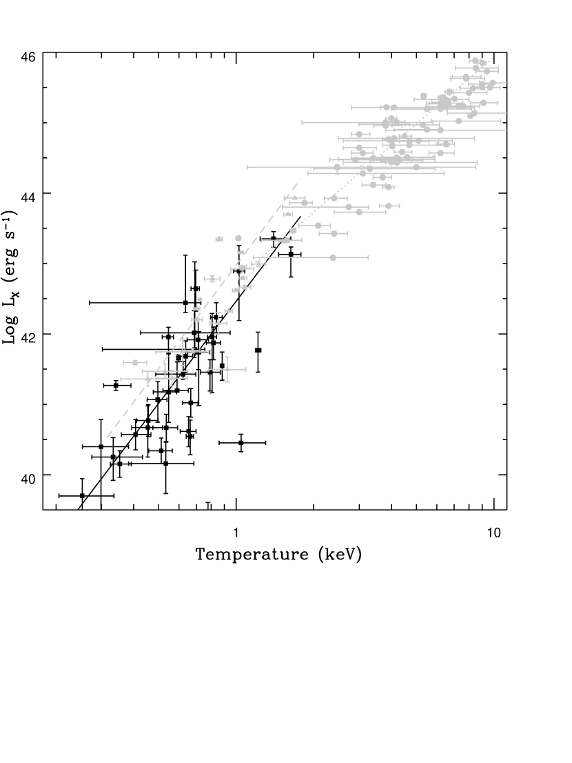
Figure 7: The $L_{\mathrm{X}}$:$T_{\mathrm{X}}$ relation for our sample, with similar relations for groups and clusters. Our galaxy data points are marked (in black) by squares, and the relation by a solid line. Group and cluster data are shown in grey. Group data are taken from Helsdon & Ponman (2000), and are marked by triangular points and a dashed line. Cluster data are drawn from David et al. (1993), Mushotzky & Scharf (1997) and Fairley et al. (2000), and are represented by circles and a dotted line. We find that the galaxy relation has a similar slope to that for groups, but is offset to fainter luminosities by a factor of $\sim$3

5.3 $L_{\mathrm{X}}$:$L_{B}$ and $L_{B}$:$T_{\mathrm{X}}$ relations

One of the more common relations used in studies of early-type galaxies is the $L_{\mathrm{X}}$:$L_{B}$ relation. Numerous studies based on ROSAT, ASCA or Einstein data have been published (e.g. Beuing et al., 1999; Matsushita, 2001; Brown & Bregman, 1998; Fabbiano et al., 1992), and we have previously examined this relation in some detail in O’Sullivan et al. (2001a), to which we direct readers for a full discussion of the relation and the effects of galaxy environment on it. Figure 8 shows the $L_{\mathrm{X}}$:$L_{B}$ relation for our galaxies. For the sample as a whole, there is a 3.9$\sigma$ correlation, with a slope of $\sim$2.7. This is quite a steep relation, comparable to that found for a sample of BGGs in previous work (O’Sullivan et al., 2001a). We have also plotted the best fit relation found for X-ray bright galaxy groups, from Helsdon & Ponman (2002). The slope of this relation (2.6$\pm$0.4) is very similar to that found for our sample of galaxies. However, our relation is offset from that for groups, with galaxies having X–ray luminosities a factor of $\sim$9 higher than those of groups with equal optical luminosity, or conversely $L_{B}$ values $\sim$2.3 times lower than groups of similar $L_{\mathrm{X}}$. This result can be compared to the $L_{\mathrm{X}}$:$T_{\mathrm{X}}$ relation shown in Section 5.2, in which galaxies are offset to lower luminosities at a given temperature, compared to groups.

Figure 8: $L_{\mathrm{X}}$ plotted against $L_{B}$ for our sample of galaxies. Although there are some outlying points, a clear trend is visible. Galaxies in X–ray bright groups are marked by circles, those in X–ray faint groups by squares. The solid line marks our best fit relation, while the dotted line shows the best fit relation for X-ray bright groups (Helsdon & Ponman, 2002).

The $L_{B}$:$T_{\mathrm{X}}$ relation for our galaxies is shown in Figure 9. Once again, for this relation we find a fairly strong correlation ($\sim$4$\sigma$ significance). The slope of the relation is comparable to that found for groups and clusters; 1.91$\pm$0.33 for our galaxy sample, 1.64$\pm$0.23 for galaxy groups (Helsdon & Ponman, 2002), and $\sim$1.5 for galaxy clusters (Lloyd-Davies & Ponman, 2002). However, where the relations for groups and clusters are essentially the same (Helsdon & Ponman, 2002), our relation for galaxies is significantly offset to higher temperatures (by a factor of $\sim$2, compared to groups) or lower $L_{B}$ (by a factor of $\sim$3).

Figure 9: $L_{B}$ plotted against temperature for our sample of galaxies. Circles mark galaxies which lie in X–ray bright groups or clusters, squares those in X–ray faint groups. The solid line is the best fit relation, while the dotted and dash-dotted lines show the relations for clusters (Lloyd-Davies & Ponman, 2002) and X-ray bright groups (Helsdon & Ponman, 2002) respectively.

5.4 The $\sigma$:$T_{\mathrm{X}}$ relation

For undisturbed objects with hydrostatic halos, both X-ray temperature and velocity dispersion should be estimators of total system mass. It should be noted that the $\sigma$ quoted for our galaxies is a stellar velocity dispersion measured in the core of each object, whereas similar relations for groups and clusters use the velocity dispersions of the galaxies within those structures. Figure 10 shows the $\sigma$:$T_{\mathrm{X}}$ relation for our sample, again subdivided by temperature structure. For the sample as a whole, we find a $\sim$3.1$\sigma$ correlation, with a slope of $\sigma\propto$$T_{\mathrm{X}}$^0.56±0.09. However, there appears to be a large degree of scatter about this line. Using the errors on the data points to measure the expected statistical scatter, we can estimate the intrinsic scatter of the data. We find that the data points are $\sim$1.8 times more scattered than would be expected from the statistical errors alone, hence the statistical scatter accounts for 56% of the variance we see.

Also marked on the plot is the best fit relation for clusters of galaxies, taken from White et al. (1999). Our relation is indistinguishable from this relation in both slope and intercept. The relation for galaxy groups is somewhat steeper; Helsdon & Ponman (2000) find a slope of $\sigma\propto$ $T_{\mathrm{X}}$^1.7±0.3 for their sample. Finally, Figure 10 shows a line representing $\beta_{spec}$=1, which is expected for systems where there is equipartition of specific energy between stars and gas. Our relation is consistent with this line, within the errors.

Figure 10: Velocity dispersion, $\sigma$, plotted against temperature for our sample of galaxies. Galaxies which show signs of central cooling are marked with open circles, those with central heating by stars, relatively isothermal galaxies by squares and those we have been unable to classify by triangles. The best fit line to the sample as a whole is marked by a solid line, and the fits to the two subsamples are marked by dashed lines. $\beta_{spec}$=1 is marked by a dotted line, while the best fit relation for galaxy clusters (from White et al., 1999) is marked by a dot-dashed line.

Although there are many previous studies of samples of early–type galaxies, very few have measured temperatures for their targets. Davis & White (1996), one of the few exceptions, fit a $\sigma$:$T_{\mathrm{X}}$ relation to a sample of 26 galaxies observed using the ROSAT PSPC or Einstein IPC. They find a slightly steeper relation than ours, with $\sigma\propto$ $T_{\mathrm{X}}$^0.69±0.1. Adding the errors in quadrature we see that their measured slope is comparable with ours, at the 1$\sigma$ confidence level. Their best fit line is however offset to higher temperature. We believe this is probably caused by contamination by surrounding emission or discrete sources, as the spectral fits use a simple one component Raymond–Smith model (Raymond & Smith, 1977). Unless the galaxies in their sample are completely dominated by halo emission, we would expect such contamination to raise the measured temperature of single component models, and we found evidence of such biases when comparing one and two component fits to galaxies in our own sample.

5.5 $\beta_{fit}$ and Entropy

Simple self–similar models of dark matter halos predict that X-ray emission from gas in the halo will always take the same form. Assuming the hot gas in the system is in hydrostatic equilibrium, the gas density can be represented by a King profile (Cavaliere & Fusco-Femiano, 1976). $\beta_{fit}$ values for groups and clusters typically lie between 0.4 and 1. Studies of low mass clusters and galaxy groups show that their surface brightness profiles become shallower with decreasing $T_{\mathrm{X}}$ (Ponman et al., 1999). This is usually taken as an indication of additional physical processes affecting the gas, the result of which is that the the gas halo appears more extended and diffuse. Self–similar models also predict that gas entropy will vary linearly with system temperature, as entropy is here defined as $S$=$T_{\mathrm{X}}$$/n_{e}^{2/3}$ (where $n_{e}$ is the electron density of the plasma), and mean gas density will be constant for all systems which virialised at the same redshift. For high mass clusters, this prediction matches the observed relation, but in lower mass systems the behaviour alters, with the trend flattening so that systems of temperature $\sim$1 keV seem to have entropy values (measured at 0.1 R_virial) scattered around a mean value of $\sim$140 keV cm² (Lloyd-Davies et al., 2000).

The most common suggested processes which could affect the gas halo are heating, either by galaxy winds (Ponman et al., 1999) or AGN (Wu et al., 2000), or cooling of very low entropy gas (Muanwong et al., 2001). Voit & Bryan (2001) have recently suggested that a combination of cooling and star formation is likely to be a highly efficient way of producing the observed effects, as the heating will be centred in regions containing the lowest entropy gas, giving the maximum entropy increase. The existence of an entropy “floor”, suggests that the level of entropy increase may be similar over a wide range of systems. In more massive systems, the entropy increase from shock heating is much larger than this amount, so it passes unnoticed. Only in small systems does it become the dominant contribution. Given this, and the fact that the suggested methods of raising the entropy are likely to occur predominantly within galaxies, we might expect that galaxy halos would show the effects of entropy increase very clearly.

The entropy floor observed in low mass systems also has an effect on their surface brightness profiles. Raising the entropy of the intra–cluster medium (ICM) through heating will push gas out to larger radii if it occurs after the system forms, or prevent it from collapsing as far as expected if it occurs beforehand. The halo will therefore be more extended, with a lower central density, presenting a flatter surface brightness profile. We therefore expect $\beta_{fit}$ to decrease with decreasing temperature, and this is observed across a wide range of systems (Ponman et al., 1999; Lloyd-Davies et al., 2000). Given the likelihood that entropy increase has occurred in galaxy halos, we may also expect to find a relation between $\beta_{fit}$ and temperature.

Figure 11 shows the slope parameter $\beta_{fit}$ plotted against temperature for our sample. There is no obvious trend in the points, and we find no statistically significant correlation. The scatter on the points is quite large, particularly at intermediate temperatures. There is no clear segregation of galaxies by temperature structure, and all classes show comparable amounts of scatter. There is some suggestion that AGN, BGGs and BCGs are more scattered than the more normal ellipticals, particularly if the normal galaxy with the highest value of $\beta_{fit}$ is excluded. This galaxy is NGC 1404, which is commonly considered to have suffered ram-pressure stripping of its halo. The sharp cut off in its surface brightness profile could conceivably have produced an unusually steep fit. However, the small size of the subsample makes any detailed comparison unreliable. The subsample seems to be centred on $\beta_{fit}\simeq$0.55, which is similar to the mean value of our sample as a whole.

Figure 11: Plots of $\beta_{fit}$ against temperature for our sample of galaxies. On the left, galaxies are grouped by their temperature properties, with those with cool cores marked by open circles, those with hot cores by stars, those with isothermal profiles by squares, and those we have been unable to classify by triangles. On the right we segregate galaxies depending on their environment, with filled triangles representing brightest group galaxies, open triangles brightest cluster galaxies, stars AGN, and squares normal early-type galaxies. Error bars are omitted for clarity.

Assuming that our galaxies are isothermal, we can extrapolate from our 2-dimensional surface brightness models to 3-dimensional density models of our galaxies. Equation 1 describes the 2D models and we can describe the 3D models as shown in Equation 3.

$$\rho_{(r)}=\rho_{(0)}[1+(r/r_{core})^{2}]^{-\frac{3\beta}{2}}$$ (3)

The density normalisation, $\rho_{(0)}$, can then be determined from the surface brightness normalisation, assuming the temperature and metallicity determined from spectral fitting. From these 3D models, it is possible to derive gas properties such as density, entropy, cooling time, etc, as a function of radius. In order to be able to compare the resulting profiles fairly, we need to view them on a common scale. This can be done by scaling the profiles by the virial radius of the system, or more usually to fixed overdensity radius, such as R₂₀₀. The overdensity is calculated relative to the critical density of the universe at the redshift of formation. This is unknown for most systems, and in the case of clusters and groups is generally taken to be the redshift of observation. For galaxies, such an assumption is very unlikely to be accurate, even taking into account the fact that early-type galaxies will have potentials determined by the density of the universe at the redshift of last major merger rather than that at which the majority of their stellar population formed. In order to calculate R₂₀₀, we assume a mean redshift of formation for ellipticals of $z_{form}$=2 (Kauffmann et al., 1996; van Dokkum & Franx, 2001). Using this value, we can calculate R₂₀₀ as described in Balogh et al. (1999) and Babul et al. (2002), taking variation of overdensity with redshift from Eke et al. (1996).

Figure 12 shows entropy, calculated at one tenth of R₂₀₀. Once again, galaxies are marked to show their different temperature structures, but while the data shows a large amount of scatter, there is no significant correlation with temperature, or segregation by temperature structure. The galaxy data points do mainly fall at the low temperature end of the S :$T_{\mathrm{X}}$ trend for groups and clusters, but show no evidence of any trend themselves.

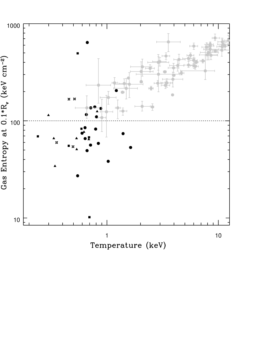
Figure 12: Mean gas entropy measured at one tenth of the virial radius plotted against mean halo temperature. Galaxies with cool cores are marked as circles, galaxies with relatively isothermal halos by squares, those with hot cores by stars and those we were unable to classify by triangles. Grey points with error bars represent groups and clusters taken from the Birmingham-CfA cluster scaling project (see Sanderson et al., 2002). The approximate level of the entropy floor for groups and clusters is marked by a dotted line.

6 Discussion

The results presented in the previous section do not lend themselves to a simple explanation. The halos of massive early-type galaxies seem to have some obvious similarities to those of galaxy groups and clusters, but also some intriguing differences. Clearly a number of the relations which hold for groups and clusters also apply to early–type galaxies, the most important examples being the $\sigma$:$T_{\mathrm{X}}$ and $L_{\mathrm{X}}$:$T_{\mathrm{X}}$ relations. The $\sigma$:$T_{\mathrm{X}}$ relation is particularly striking, in that it agrees closely with the relation found for galaxy clusters. The $L_{\mathrm{X}}$:$T_{\mathrm{X}}$ relation has a similar slope to that of galaxy groups, but is offset to lower luminosities. The $L_{B}$:$T_{\mathrm{X}}$ and $L_{\mathrm{X}}$:$L_{B}$ relations also show offsets from the cluster and group relations, but to higher X–ray luminosity and temperature. Another important result is the roughly constant value of $\beta_{fit}$ across a wide range of temperatures. Although there is some suggestion of influence by surrounding groups and clusters on this parameter, the environment seems to increase scatter rather than producing a trend. Together with the results of our entropy calculations for the sample, the behaviour of $\beta_{fit}$ suggests that if preheating effects are important in galaxy halos, they produce results quite different to those seen in groups.

6.1 Comparison with Groups and Clusters

One of the most important results to arise from studies of galaxy groups and clusters is the demonstration that simple self-similar models do not describe low mass systems well. There is good evidence that galaxy groups differ from higher mass clusters in a number of important ways. The most widely accepted explanation for these differences is that the hot gas in the halos of these systems is affected not only by the processes involved in formation of the system as a whole, but also by processes such as star formation, AGN heating, and gas cooling. A clear sign of this is seen in the behaviour of gas entropy in systems of different mass. In high mass clusters, entropy can be fairly accurately predicted from simple models in which the gas is heated (and has its entropy profile set) during formation of the system. As the cluster builds up, gas flows into the potential well and is shock heated to a degree dependent on the depth of the potential. This dependence of halo temperature on system mass can be seen in the $\sigma$:$T_{\mathrm{X}}$ relation for clusters, in which $T_{\mathrm{X}}$ is strongly correlated with $\sigma$, with $T_{\mathrm{X}}$ $\mathrel{\hbox to0.0pt{\lower 3.0pt\hbox{$\sim$}\hss}\raise 2.0pt\hbox{$\propto$}}$  $\sigma^{2}$, as expected from arguments based on the virial theorem.

However, as system mass (and temperature) drop, the gas entropy begins to depart from the predicted relation, with low mass galaxy groups having higher than expected gas entropies. Lloyd-Davies et al. (2000) have shown that at temperatures below $\sim$2 keV, gas entropy appears to remain roughly constant, scattering about a mean value of 140 keV cm². An effect is also seen at around this temperature in the surface brightness profiles of galaxy groups and clusters (Ponman et al., 1999). High temperature systems ($T_{\mathrm{X}}$ $>$ 4 keV) have profiles which scale self-similarly, but as $T_{\mathrm{X}}$ is lowered, the surface brightness profiles observed are found to be shallower, with lower central densities. This has an obvious effect on the measured X–ray luminosities of these systems, making them fainter than predicted.

Both of these trends are explained through the effects of non-gravitational processes on the gas. To take a simple model, we can imagine a system at the time of formation. As stated above, we expect the gas falling into the potential of the system to be heated by gravitational processes, but we might also expect heating from other sources. For example, as galaxies form in the system we could expect star formation, galaxy winds, and AGN to affect the gas in the system halo. In a large system, the contribution from these sources will be small compared to that of gravitational heating. However, in smaller systems it will be more important, and will eventually dominate the energy of the gas halo. This additional heating will have a number of effects, such as raising the gas temperature, causing the halo to expand by moving gas to higher radii, raising the entropy of the gas, and so on. In practice, it is possible to achieve these effects through a number of processes, or a combination of several. One promising model is that of Voit & Bryan (2001), in which low entropy gas cools rapidly, providing material for star formation. This star formation then not only removes low entropy gas from the system (raising the mean entropy), but provides heating which is focused in the areas in which low entropy material dominates. From our point of view however, the method is not important; all the suggested processes would occur in galaxies, and might be expected to occur preferentially in large galaxies at the bottom of a group or cluster potential well. For simplicity, we will refer to this as the preheating model.

6.1.1 The $\sigma$:$T_{\mathrm{X}}$ relation

One of the clearest similarities between the relations for our galaxies and those of larger structures is the correspondence of the $\sigma$:$T_{\mathrm{X}}$ relation to that of galaxy clusters. As discussed above, the correlation in clusters is expected, and shows that both $T_{\mathrm{X}}$ and $\sigma$ are good measures of the potential. In galaxy groups, the slope of the relation is observed to be somewhat steeper, $\sim$1.7$\pm$0.3 (Helsdon & Ponman, 2000). One explanation for this steeper slope is that $T_{\mathrm{X}}$ is raised in low mass systems by the heating and removal of cool gas described above. An alternative is the suggestion that the velocity dispersions measured in groups could be biased. There are a number of groups which, despite apparently possessing extended X-ray halos, have exceptionally low velocity dispersions (Helsdon & Ponman, 2000). If these $\sigma$ values were accurate, the potential of the group would not only be too shallow to produce the halo luminosity observed, but would be too shallow for the group to have collapsed within the age of the universe. Several reasons for underestimation of $\sigma$ can be postulated. It is possible that these low mass groups form a central core of bright galaxies, with fainter members at higher radii. The brightest galaxies are most likely to be recognised as group members and have measured redshifts, so they will dominate any calculation of $\sigma$. Tidal interactions between group members could reduce velocity dispersion by transferring orbital energy from the galaxies to their stars. It has also been suggested that low mass groups may be biased because the groups often have prolate structures. For groups whose major axis lies near the plane of the sky, this particular structure could lead to an underestimation of $\sigma$ (Tovmassian et al., 2002), biasing samples including such low temperature systems. If $\sigma$ is biased, correcting the measurements for the lowest temperature groups would probably shift the best fit relation into agreement with that seen in clusters. It is worth noting that the groups with the lowest velocity dispersions listed in Helsdon & Ponman (2000) are also amongst the poorest; all groups in their sample with $\sigma<$ 150 $\mbox{~{}km}\mbox{~{}s}^{-1}$ have only 3-5 member galaxies. Calculating velocity dispersion from such small numbers can introduce a bias, producing values which are underestimated by up to 15% (Helsdon, 2002).

The fact that our results agree well with the cluster relation suggests that again, we are looking at systems in which both $T_{\mathrm{X}}$ and $\sigma$ are good measures of the potential. From a preheating point of view this is surprising. If we expect preheating processes to occur in large galaxies, then we might expect the $T_{\mathrm{X}}$ of their halos to be raised, in much the same way as we see in galaxy groups, producing a steeper relation. We also need an explanation of why the gas in these galaxies has a temperature which is related to the depth of their potential well. As well as additional heating from star formation and AGN activity, we expect large quantities of gas to be lost from the stars in the galaxy. As this gas is produced within the galaxy, we cannot expect shock heating during infall, so we might initially believe its temperature to be entirely determined by supernova heating.

Helsdon et al. (2001) consider a related question, that of the relative importance of different energy sources which contribute to the total X–ray luminosity of early–type galaxies. Their Figure 8 is a plot of $L_{\mathrm{X}}$/$L_{B}$ against $L_{B}$, showing the contributions to $L_{\mathrm{X}}$ from discrete sources, SNIa and gravity. From our point of view the contribution from discrete sources is irrelevant, as we are interested in energy input to the gas in the galaxy. The gravitational contribution is a combination of two processes, firstly a contribution from the velocity of the stars in the potential (gas lost from these stars will have an added kinetic energy component from their velocity, which will be thermalized in the surrounding ISM), and secondly a contribution from work done on the gas as gravity causes it to contract and cool. The important result with regards to our situation is that while the SNIa energy input scales with $L_{B}$, the gravitational input scales with $\sigma^{2}$. This means that for low mass systems, the dominant contribution to $L_{\mathrm{X}}$ is from supernova heating, but above $L_{B}$ $\sim$ 10¹⁰ $L_{\odot}$ gravitational work begins to dominate. If we consider these two factors as energy inputs to the gas rather than as contributors to $L_{\mathrm{X}}$, we can see that the gas temperature is likely to be determined by the supernova rate in low mass systems, and by the depth of the potential in high mass systems. The point at which the two are equal will depend on the details of the model, but if we follow the assumptions made by Helsdon et al. (2001), all our galaxies lie in the high mass, gravitationally dominated region of the plot. We could therefore expect gas temperature to depend on the depth of the potential, whether the gas has an internal or external origin.

It seems likely, from this result, that we can draw similar conclusions from the $\sigma$:$T_{\mathrm{X}}$ relation in galaxies as we would in clusters. $T_{\mathrm{X}}$ and $\sigma$ are both probably good measures of mass. Preheating, by whatever method, does not appear to have the effect on galaxy halos that it has on those of groups. Like clusters, the galaxy relation is consistent with the systems having $\beta_{spec}$ = 1, suggesting that there is equipartition of specific energy between stars and gas. As we will discuss later, this has important implications, in that it suggests that the optical and X–ray density profiles should be similar. One further consideration is the intrinsic scatter in the points. Our data has $\sim$1.8 times as much scatter as we would expect from statistical errors alone, giving us a non-statistical unceratinty in T of $\pm$0.04 for any given value of $\sigma$. For comparison, the galaxy groups studied by Helsdon & Ponman (2000) are less scattered, having only $\sim$1.4 times as much as would be expected from the errors, sothe non-statistical uncertainty in T for these systems is $\pm$0.86. The degree of scatter in the galaxy data could have a number of causes. Gas temperature could be affected by many processes, related to the galaxy or the surrounding environment. Velocity dispersion could also be affected by processes associated with the formation or merger history of the galaxy. However, it would appear that galaxy groups have a larger scatter in properties, suggesting that the galaxies are less affected by external influences.

6.1.2 The $L_{\mathrm{X}}$:$T_{\mathrm{X}}$ relation and $\beta_{fit}$

Accepting $\sigma$ and $T_{\mathrm{X}}$ as indicators of the mass of the system, we next consider the $L_{\mathrm{X}}$:$T_{\mathrm{X}}$ relation. Here, we find that the slope of the relation is steeper than that of clusters, as steep as that of groups. The relation is also offset, so that at a given temperature, galaxies have a lower luminosity than groups. The steep slope is usually explained as a product of preheating - the additional heating of the gas raises the temperature slightly and moves gas to higher radii, lowering the central density and therefore $L_{\mathrm{X}}$. If we assume that the steep slope seen in galaxies is caused by the same processes which cause it in groups, then this relation is a strong piece of evidence for the effects of preheating in galaxies.

However, there are other ways in which we might produce such a steep slope. Helsdon et al. (2001) found a strong correlation between the X–ray properties of group dominant galaxies and those of the groups in which they are found. Given the signs of central cooling in many of these groups, they suggested that what had been initially identified as the halos of the dominant galaxies were in fact group scale cooling flows, centred on the dominant galaxy because it lies at the bottom of the group potential. They also found that the $L_{\mathrm{X}}$ of this central galaxy halo/cooling flow was $\sim$25% of the $L_{\mathrm{X}}$ of the group. As 29 of our 39 galaxies are dominant galaxies in groups, clusters or cluster subclumps, we must consider the idea that our relations could be dominated by cooling flows. In that case, we would expect the $L_{\mathrm{X}}$:$T_{\mathrm{X}}$ relation to have a similar slope to that of groups, but to be offset to lower $L_{\mathrm{X}}$ values by a factor of 4, and also to lower temperatures. Provided the temperature drop is not too large, this could reproduce the relation we see very well. On the other hand, we do not see any segregation in the data between those galaxies which show signs of central cooling and those which do not, nor do we see any difference between galaxies at the centres of groups and those in other environments. This argues against cooling flows as the driver of the relation. We will discuss the evidence for and against cooling flows as the dominant factor in Section 6.2.

The lack of a relation between $\beta_{fit}$ and $T_{\mathrm{X}}$ argues against both cooling flows and preheating as the source of the $L_{\mathrm{X}}$:$T_{\mathrm{X}}$ relation. In galaxy groups, preheating causes gas to move out to high radii, reducing $\beta_{fit}$ as the surface brightness profile becomes flatter. As preheating is more effective in smaller mass systems, groups and low mass clusters show a correlation between $\beta_{fit}$ and $T_{\mathrm{X}}$  with cooler systems having flatter profiles. In galaxies, despite a very large scatter, we see no trend with temperature. Our galaxies lie around a mean value of $\beta_{fit}$ = 0.55, which means that even if the group and cluster $\beta_{fit}$:$T_{\mathrm{X}}$relation levelled off at low temperature, our sample would not be consistent with it. This strongly suggests that preheating is not the cause of the steep slope of the $L_{\mathrm{X}}$:$T_{\mathrm{X}}$ relation.

If a change in the slope of the surface brightness profile is not responsible for the drop in $L_{\mathrm{X}}$ needed to produce the $L_{\mathrm{X}}$:$T_{\mathrm{X}}$ relation, then there must be a drop in normalisation. This is demonstrated in Figure 13, which shows the surface brightness profiles of our sample, scaled so that if they were behaving self-similarly, they would coincide. Details of this scaling are given in the figure caption.

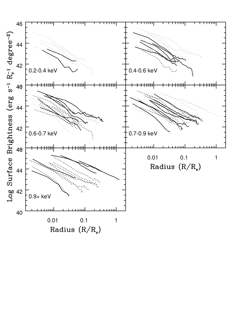
Figure 13: Scaled X-ray surface brightness profiles for our galaxies, arranged to show departures from self-similarity. The profiles have been scaled to the virial radii of the galaxies (assuming a redshift of formation $z_{form}$=2), and by $T_{\mathrm{X}}$^1/2 to account for self-similar scaling with mass (Ponman et al., 1999). We have also converted from counts to intensity, using the best fit MEKAL component of each galaxy to allow for the temperature and metallicity dependence of the plasma emissivity. As all our galaxies are at low redshift ($z<$ 0.035) we ignore cosmological effects as negligible. In each plot bold, dark lines show the galaxies in the energy band in question, narrow, grey lines show those in the band above, and dotted lines those in the band below. Although there is some scatter, it is clear that all have similar slopes and that cooler systems have lower normalisations.

A comparison between Figure 13 and Figure 1 of Ponman et al. (1999) demonstrates the difference between the behaviour of our galaxies and that of groups and clusters. The high temperature clusters in Figure 1 of Ponman et al. (1999) behave self-similarly, having roughly equal surface brightness slopes and scaled normalisations. The lower temperature groups move away from self-similarity, as their slopes flatten and central surface brightness (and density) is lowered. In the galaxies, although there is a large amount of scatter, the slope remains roughly constant across the range of temperatures, but the normalisation of the profiles seems to drop with decreasing temperatures. This suggests that whereas in galaxy groups the steepening of the $L_{\mathrm{X}}$:$T_{\mathrm{X}}$ relation is caused by energy injection and movement of gas to higher radii, in galaxies is caused by changes in normalisation and therefore in the overall gas fraction of the systems. The processes responsible for this change are not clear, but this result demonstrates how differently galaxies behave compared to groups and clusters.

It is interesting to note that the mean slope of the surface brightness profiles ($\beta_{fit}$ = 0.55) is similar to the mean slope of the optical surface brightness profile. Elliptical galaxies are well described in the optical by a de Vaucouleurs profile, which is similar (outside the central regions) to a King model with $\beta_{fit}$ = 0.5. As mentioned in Section 6.1.1, the $\sigma$:$T_{\mathrm{X}}$ relation is consistent with $\beta_{spec}$ = 1, which leads us to expect a similarity between the optical and X-ray density profiles. The similarity in surface brightness profiles is therefore further confirmation of the $\sigma$:$T_{\mathrm{X}}$ result. A further interesting note is that galaxy wind models, in which the majority of the gas in the halo is produced by stellar mass loss, predict X–ray surface brightness profiles similar to those in the optical (Pellegrini & Ciotti, 1998). The exact value of $\beta_{fit}$ would depend on the wind state of the system, with only relatively hydrostatic halos having $\beta_{fit}$ = 0.5. Galaxies dominated by supersonic outflows, or those in which inflows are important, would be expected to have steeper profiles owing to their high central gas densities. Galaxies dominated by subsonic outflows would be expected to have slightly flatter profiles ($\beta_{fit}$ $<$ 0.5), as the outflowing gas has a higher density at large radii than in a supersonic flow, and less of a central peak. If such models are applicable, it seems likely from the high mass of our galaxies that they would be in the inflow stage, so we would expect $\beta_{fit}$ $>$ 0.5, in agreement with our observations.

6.1.3 Entropy

The results of our entropy measurements are in broad agreement with those from the surface brightness profiles. In galaxy clusters and groups we see evidence of similarity breaking and preheating, leading to a trend in entropy which levels off at the entropy floor. The galaxy data points do not show any sign of a trend, and although they may appear to be consistent with the general trend in higher mass systems, the scatter in the data is very large. Our method of calculating entropy has two important sources of scatter associated with it. Firstly, we must assume that our galaxies are isothermal, despite the fact that we know that many of them have temperature gradients. Secondly, we measure the entropy at one tenth of the virial radius, and when calculating the virial radius we must assume a redshift of formation (or last major merger). Although the assumed value of $z_{form}$ = 2 is probably a reasonable mean, there will clearly be variation between individual galaxies. Our virial radii will therefore be inaccurate to some degree, meaning that we are actually measuring entropy at a range of scaled radii.

Despite these difficulties, we can draw some important results from the entropy values. A large proportion of the data points lie below 100 keV cm², meaning that they are below the entropy floor observed in galaxy groups. One possible reason for these low values is that the galaxies form earlier than the surrounding groups. The density of systems virialising at a given epoch is related to the critical density of the universe at that time, and so the earlier an object virialises, the denser we expect it to be. As entropy is inversely proportional to $n_{e}^{2/3}$, an equal amount of energy injected into a denser system will produce a smaller increase in entropy. Galaxies, forming at $z$ $\sim$ 2, might therefore be expected to have higher densities and a lower entropy floor than groups and clusters which have formed more recently. However, we might also expect that as the site of the processes responsible for entropy increase, the amount of energy available to affect entropy in galaxies would be larger than in groups. It is also worth considering that if galaxies had formed with halos of very low entropy gas, it would have cooled on timescales considerably shorter than the Hubble time, probably leading to star formation, heating and a rise in observed entropy (Voit & Bryan, 2001).

An alternative viewpoint is that the majority of the gas in these systems is being produced by stellar mass loss rather than infall, so we should not expect entropy to behave as it does in groups. In this case, galaxy wind models should give a reasonable approximation of the behaviour of the halo, in the absence of significant environmental influences. Several published simulations of galaxy halo development give gas density and temperature profiles (Ciotti et al., 1991; Pellegrini & Ciotti, 1998; Brighenti & Mathews, 1999) for their model galaxies. In models of outflowing winds, both gas density and temperature fall with radius, but density falls more rapidly, so we would expect an entropy profile which increases with radius. In models which have developed gas inflow (cooling flows), temperature may rise with radius throughout most of the model, so again we expect entropy to rise with radius. This matches what we observe in our measured entropy profiles. The entropy predicted at any given radius depends on the details of the model, e.g.  system mass, age, supernova rate, mass injection rate, etc. Entropies ranging from 20-300 keV cm² might be expected for galaxies such as those in our sample. The majority of our galaxies do have entropies within these limits, and considering the expected scatter, the agreement between models and measurements is fairly good.

6.2 Cooling Flows

A number of our galaxies have temperature profiles indicative of central cooling. This is not surprising, as they are fairly massive objects, with large halos, and reside within larger structures which are themselves probably capable of producing cooling flows. Among the relations we have examined, several show behaviour which could be explained easily as the product of group cooling flows. The best example of this is the $L_{\mathrm{X}}$:$T_{\mathrm{X}}$ relation, where the slope is identical (within errors) with that found for groups, but offset to lower X-ray luminosities. As discussed in Section 6.1.2, this offset (a factor of 3 in $L_{\mathrm{X}}$) is very similar to that we would predict (a factor of 4), based on studies of X-ray bright groups (Helsdon et al., 2001). We would expect the measured $T_{\mathrm{X}}$ of the cooling flow region to be lower than the group temperature and this could explain the difference between predicted and measured offset. We might also be able to explain the offsets observed in the $L_{\mathrm{X}}$:$L_{B}$ and $L_{B}$:$T_{\mathrm{X}}$ relation using this model. In both cases we are comparing a parameter which is determined by the galaxy and only weakly influenced by the group ($L_{B}$) to a parameter which is determined by the cooling flow and hence by the properties of the group ($L_{\mathrm{X}}$ or $T_{\mathrm{X}}$). In such a situation, we would have to expect $L_{\mathrm{X}}$ and $T_{\mathrm{X}}$ to appear unusually high for the central galaxy, as they would actually be related to the much larger system of the surrounding group or cluster. Comparing with optical luminosity, we would only expect to find a relation without an offset if we compared them to a value of $L_{B}$ calculated for all the galaxies in the group, rather than just the central dominant elliptical. We would also expect the galaxies in X–ray faint groups to behave differently, as their halos could not be the product of group scale cooling flows. Unfortunately, the small numbers of such objects in our sample means we cannot test whether they follow a different trend to those in X–ray bright groups, but they do indeed appear to fall at lower $L_{\mathrm{X}}$ and $T_{\mathrm{X}}$, for a given $L_{B}$.

However, there are two powerful arguments against group scale cooling flows as the dominating influence in our sample. Firstly, we find that a significant subset (one third) of our sample do not show signs of central cooling. They are instead approximately isothermal, or have a central rise in temperature. This does not necessarily mean that they have not been at the centre of a group cooling flow in the past, but such a flow would have to have been disrupted, and so would be unlikely to produce the emission we assume to be a halo. Secondly, and most importantly, we see no sign of a difference between those galaxies with or without signs of central cooling. The only segregation we see in any of the relations is a tendency for galaxies which seem to harbour cooling flows to be higher mass systems, and so to have higher values of $\sigma$, $T_{\mathrm{X}}$, $L_{\mathrm{X}}$, etc. We see no other difference between galaxies with differing temperature profiles, and we specifically do not see the galaxies with apparent cooling flows driving the $L_{\mathrm{X}}$:$T_{\mathrm{X}}$ relation. This strongly suggests that while a number of our galaxies do harbour cooling flows, some of them quite large, their halos are not simply cooling flows formed by surrounding groups and clusters, unless the properties of the gas halo are independent of whether it arises from stellar winds or group inflow.

6.3 Stellar Mass Loss and Galaxy Winds

Large scale cooling flows, in which most of the gas in the galaxy halo has an external origin, do not appear to provide a good model for our galaxy sample. The alternative is a model in which the majority of the gas is produced (and heated) internally, via stellar mass loss. We have already discussed in Section 6.1.1, the relative contributions to the energy of gas produced in a galaxy from supernovae and gravitational processes. Our sample is made up of galaxies with high stellar masses, leading us to believe that the gravitational potential should be the dominant source of energy. This provides an important link between the X–ray properties of the galaxies and their mass, which could explain the correlations we see between optical and X–ray properties in our sample. If gravity is the dominant source of energy in the halos of our galaxies, we would expect them to behave like clusters on many of the relations we have examined. The best example of this is the $\sigma$:$T_{\mathrm{X}}$ relation, where the galaxies and clusters have best fit lines which are indistinguishable.

However, there are a number of ways in which the relations do not behave like those of galaxy clusters, and we need to find explanations for these differences. The most interesting, and perhaps the most important, is the $L_{\mathrm{X}}$:$T_{\mathrm{X}}$ relation. This behaves like that of galaxy groups, rather than galaxy clusters. However, instead of a decrease in central gas density in low mass systems, leading to a trend in $\beta_{fit}$ with temperature, we see a constant value of $\beta_{fit}$ and a decrease in the normalisation of the surface brightness profiles at low masses. This suggests that the lower mass members of our sample lie progressively further below the cluster $L_{\mathrm{X}}$:$T_{\mathrm{X}}$ relation because they have a lower gas fraction than their higher mass counterparts. To explain the $L_{\mathrm{X}}$:$T_{\mathrm{X}}$ relation we observe, we need an explanation of this change in gas fraction with temperature.

A number of possible reasons for this trend in gas fraction ($\mathit{f}_{gas}$) could be suggested. These include:

1. The change in $\mathit{f}_{gas}$ is a natural consequence of halo production by stellar mass loss. Any steady state solution would produce the trend we see.

2. The change in $\mathit{f}_{gas}$ is the product of the surrounding environment. Higher mass systems tend to be in higher mass groups and clusters, which have a denser IGM. This prevents the escape of gas, or compresses the halo, or allows accretion of gas, causing the halo to reach higher densities and gas fractions.

3. The lower gas fraction in cooler galaxies is an evolutionary effect, related to the age (or time since last major merger) of the galaxy. The mass density of the system is determined by the density of the universe at the time at which the system collapsed (or underwent its last major merger), so the older systems have the highest density and are therefore the hottest.

4. Supernova heating, though not the dominant source of energy in the halos, does have a second order effect on them. Perhaps in lower mass systems, the relatively higher contribution from SNIa causes gas to be lost from the potential, lowering the overall fraction.

Of these suggested models, the last seems the least likely. Although it is plausible that supernova heating could have observable effects on the galaxy halos, particularly in the least massive members of our sample, it seems unlikely that it could affect the gas fraction in the same way at all radii. In the analogous situation of gas heating in galaxy groups, the central gas fraction is lowered, but only by moving gas to higher radii, raising the gas fraction there. There are however some obvious differences which could make this comparison invalid, such as the distributed heating and mass injection expected from the stars in a galaxy. It is also important to remember that we cannot in most cases observe the galaxy halo to high radii. It is possible that gas could be removed to a large fraction of the virial radius, where its low density might make it undetectable, and where it could be easily stripped by any interaction with a surrounding IGM. However, the fact that we see no sign of any trend in $\beta_{fit}$ is a strong argument against this hypothesis.

There are also problems with the idea that such a trend might be a natural result of galaxy halos forming from gas of stellar origin. Previous work on a larger sample including galaxies found in a variety of environments and with a wide range of luminosities suggests that galaxy winds are the most likely formation method for the halos of early–type galaxies of all sizes (O’Sullivan et al., 2001b, a). However, these studies also confirmed that large group or cluster dominant ellipticals, such as those in our sample, have X–ray properties which differ significantly from those of less massive galaxies. They could therefore be the most likely group of objects to form their gas halos through some other mechanism. Our results suggest that the steep trend in the $L_{\mathrm{X}}$:$T_{\mathrm{X}}$ relation is caused by the drop in $\mathit{f}_{gas}$ and hence $L_{\mathrm{X}}$. The $L_{\mathrm{X}}$:$L_{B}$ relation also has a steep slope compared to that of non–BGG ellipticals (O’Sullivan et al., 2001a), and it seems likely that this is again a product of the trend in $\mathit{f}_{gas}$ with temperature. If so, we cannot argue that the trend in gas fraction is a product of halo formation by galaxy winds, as we would expect all galaxies to show a steep $L_{\mathrm{X}}$:$L_{B}$ relation, as seen for this sample.

A change in gas fraction caused by the different formation histories of the galaxies seems a more feasible model. Assuming our galaxies have formed through a number of mergers, we can assume that there is a scatter in the time since the last major merger. While minor mergers can be treated as the accretion of extra matter into the galaxy, major mergers will have more profound effects, including the “resetting” of the potential well through violent relaxation (Salvador-Sole et al., 1998) and the fuelling of bursts of star formation. Luminosity weighted ages (based on comparing optical absorption line indices to stellar population models) tend to be dominated by any young component in the stellar population, so that if the galaxy has formed part of its stellar population through a merger and starburst, the age measured is likely to be an estimate of the time since that merger. In a previous paper (O’Sullivan et al., 2001b) we found a relation between the luminosity weighted age of a sample of 77 early–type galaxies in a range of environments and their normalised X–ray luminosity, $L_{\mathrm{X}}$/$L_{B}$. This indicates that the halo luminosity of such galaxies increases as they age. In galaxy wind models, this can be explained through the transition from rapid outflows to slower winds or inflows, during which the halo density and the gas mass in the potential well increases.

The question then becomes whether we expect the more massive galaxies in this sample to have had their last major merger earlier, and therefore to have higher halo densities. Hierarchical models of galaxy formation predict that more massive galaxies have longer formation timescales (Kauffmann, 1996), suggesting that this is not the case. However, observational measurements of age for sample of galaxies in clusters and the field suggest that more massive galaxies do indeed form earlier (Thomas et al., 2002). In our previous study of X–ray variations with galaxy age we found no correlation between $L_{B}$ and age (O’Sullivan et al., 2001b), but in that case our sample included galaxies from a much wider range of environments and with more varied luminosities than is the case in this paper. In the current sample only 16 of our galaxies have measured ages in the catalogue of Terlevich & Forbes (2002), and for this subsample we find only a weak (1.4 $\sigma$) trend for age to increase with $L_{B}$. We are therefore unable to say whether merger history is the deciding factor in determining gas fraction, though it does seem possible.

Finally there is the possibility that the change in gas fraction we see is related to the environment of the galaxies. The offsets we see in the $L_{\mathrm{X}}$:$L_{B}$ and $L_{B}$:$T_{\mathrm{X}}$ relations suggest that the presence of a surrounding IGM can increase the X–ray luminosity and temperature of the halo. $L_{\mathrm{X}}$ appears to be more strongly affected, being offset by a factor of $\sim$9, as compared to a factor of $\sim$2 in $T_{\mathrm{X}}$. A surrounding IGM might cause these offsets by containing or stifling galaxy winds, or by through accretion of the IGM on to the galaxy halo. If the most massive galaxies were found in the most massive groups and clusters we might expect the density of the surrounding IGM to correlate with galaxy mass. This would mean that more massive systems were more strongly affected, and might produce the trend in gas fraction with temperature. Of the possible processes, containment or stifling would seem the most likely, as accretion of IGM gas might be expected to affect gas fraction differently at different radii. One strong argument for this explanation is the correlation between group and galaxy X–ray luminosity observed by Helsdon et al. (2001). If we assume that this is not caused by group cooling flows then it does indeed suggest that galaxy mass is correlated with group mass.

6.4 Environmental Effects and Formation Epoch

Although most of the relations which we have used to investigate our sample of galaxies show no difference between galaxies in different environments, there are three interesting exceptions. These are the $L_{B}$:$T_{\mathrm{X}}$, $L_{\mathrm{X}}$:$L_{B}$ and $\beta_{fit}$:$T_{\mathrm{X}}$ relations. The $L_{B}$:$T_{\mathrm{X}}$ and $L_{\mathrm{X}}$:$L_{B}$ both show similar behaviour. In each case, we find that the best fit relation has a similar slope to that of groups, but is offset to higher $L_{\mathrm{X}}$ or $T_{\mathrm{X}}$ at a given $L_{B}$. However, when we split the sample into galaxies which lie in X–ray bright or X–ray faint groups, we find that those in X–ray faint groups do not appear to be offset to the same degree. We have calculated the residuals about our best fit lines for both relations, and the residuals we would find if the best fit lines for galaxy groups were used. In both cases, the mean residual from our best fit line is considerably higher (by 20-30%) for the galaxies in X–ray faint groups than for those in X–ray bright groups, showing them to be poorly described by the relations. The points are almost all offset toward the group relations, so these large residuals are a measure of that offset. We can also calculate the mean residual from the group relations, which will give us a measure of the offset of the X–ray faint and bright subsets from those relations. The mean residual from the best fit line for groups is smaller (by 40-60%) for galaxies in X–ray faint groups. For the $L_{\mathrm{X}}$:$L_{B}$ relation, the mean residual of the galaxies in X–ray faint groups from the group relation is actually less than half the mean residual from the galaxy best fit line, suggesting that although these galaxies are not well described by either relation, they are closer to the group relation. This supports the idea that the offset is driven by the presence of a surrounding IGM. Alternative subdivisions of the sample, comparing cooling flow and isothermal galaxies, or group dominant galaxies to those in other environments do not show a similar segregation, leading us to the conclusion that this difference is not a product of group cooling flows.

There are a number of ways in which a surrounding IGM could increase the luminosity and temperature of a galaxy halo. If we consider a galaxy in an early wind phase, the rapidly outflowing gas might expand until stopped by the pressure of the surrounding gas. The IGM could contain the galaxy wind, raising its density and preventing the dispersion of high temperature gas to large radii. We might therefore expect such an object, even if it has now progressed to a later wind phase, to have a higher temperature and luminosity. Similarly, if we consider a galaxy in which there is a global inflow (within the galaxy halo rather than a group cooling flow initially sourced in the surrounding IGM), we might expect gas from the IGM to move into the galaxy potential. This gas would add to the galaxy luminosity, particularly as the galaxy potential would concentrate it. We might also expect it to have a higher temperature than gas produced within the galaxy. In both cases we might also see an increased amount of gas in the galaxy at all radii. If the trend in gas mass fraction discussed in Section 6.1.2 is caused by an increase in halo density for high temperature systems (rather than a density decrease in low $T_{\mathrm{X}}$ galaxies), these models might give us an explanation of the trend. More massive galaxies would produce larger amounts of gas and would be more able to accrete and concentrate a surrounding IGM, so we would expect the trend with temperature.

The other sign of environmental influence on our galaxies is shown in Figure 11. If we exclude NGC 1404 (where $\beta_{fit}$ is likely to be biased by the effects of ram-pressure stripping), we find that galaxies in the centres of groups, clusters and cluster sub-clumps show a larger degree of scatter in $\beta_{fit}$ than those elsewhere. In this case the trend seems to be related to the position of the galaxy at the centre of the potential well rather than a surrounding or confining IGM. All the non-BGG/BCG galaxies in our sample are found in groups or clusters, so their halos are likely to interact with surrounding gas. A possibility is that the halos of galaxies at the centres of larger structures are affected by the group potential, rather than the IGM. A recent study of NGC 1399 (Paolillo et al., 2002) shows that in the central regions of that galaxy (the dominant elliptical of the Fornax cluster), the mass profile is dominated by the stellar mass of the galaxy. However, the cluster potential does play some part at larger radii, and although we have removed the surface brightness components associated with larger structures, we cannot rule out some level of influence. Another possibility is that the merger history of these central galaxies has an effect on their halo structure. Dynamical friction is thought to cause galaxies in groups and clusters to lose orbital energy and fall towards the centre of the potential. We might therefore expect to find that group and cluster central galaxies undergo many more mergers than galaxies elsewhere. The associated disturbance, influx of gas, and star formation might produce effects which can change the state of the galaxy halo, inducing the scatter we observe.

Although environmental influences seem likely, and provide an explanation for the offsets seen in the $L_{B}$:$T_{\mathrm{X}}$ and $L_{\mathrm{X}}$:$L_{B}$ relations, this model raises further questions, when compared to the other relations. There is a discrepancy between the $\sigma$:$T_{\mathrm{X}}$ and $L_{B}$:$T_{\mathrm{X}}$ relations. In the $\sigma$:$T_{\mathrm{X}}$ relation, temperature appears to be a good measure of mass, with a behaviour similar to that seen in galaxy clusters. In the $L_{B}$:$T_{\mathrm{X}}$ relation we see an offset, suggesting that while $T_{\mathrm{X}}$ may be a good measure of mass, either galaxies have higher temperatures than clusters at a given mass, or that they have lower optical luminosities. If we accept the $\sigma$:$T_{\mathrm{X}}$ relation, we must assume that the offset is in $L_{B}$, and at first glance this suggests that galaxies have a higher mass-to-light ratio than clusters. This is rather unexpected, as cosmological simulations suggest that mass-to-light ratio is correlated with dark halo mass, with galaxy clusters having considerably higher mass per unit $L_{B}$ than individual galaxies (Somerville et al., 2001). A similar discrepancy is seen between the $L_{\mathrm{X}}$:$T_{\mathrm{X}}$ and $L_{\mathrm{X}}$:$L_{B}$ relations, in which the former has an offset to lower $L_{\mathrm{X}}$ (or higher $T_{\mathrm{X}}$), while the latter has an offset to higher $L_{\mathrm{X}}$ (or lower $L_{B}$). Once again, if we assume temperature behaves as it does in clusters, then the $L_{\mathrm{X}}$:$T_{\mathrm{X}}$ relation suggests that $L_{\mathrm{X}}$ is reduced, relative to larger structures. The offset in the $L_{\mathrm{X}}$:$L_{B}$ relation would then again imply a large reduction in $L_{B}$, compared to groups and clusters. It is not clear what is causing these offsets, but we can speculate to some extent.

One possibility to be considered is the difference in formation epoch between galaxies, groups and clusters. Although properties such as $\sigma$ and X–ray temperature can be considered as measures of system mass, they are actually related to the depth of the potential well ($T_{\mathrm{X}}$ $\propto$ M/R). We expect systems to have densities related to the critical density of the universe at the time at which they virialise (or undergo their last major merger), so systems of a given mass which form at earlier epochs should have deeper potentials than their more modern counterparts. This suggests that older systems will have higher velocity dispersions, X–ray temperatures and luminosities than younger ones. A comparison of systems of different ages should show these differences, and relations involving these parameters would be affected them. Relations involving optical luminosity might show them particularly well, if the total stellar luminosity is related to system mass rather than the depth of the potential well.

As we are considering similar systems at different redshifts, we take the total mass, $M_{tot}$ to be constant, but the radius of the system is reduced at higher redshift, R $\propto$ (1+$z$)^-1. Therefore, density scales as

$$\rho_{tot}\propto\frac{M_{tot}}{R^{3}}\propto(1+z)^{3},$$ (4)

as expected. We also know that for bremsstrahlung radiation, the luminosity can be written

$$L_{X}\propto\rho_{tot}^{2}R^{3}\sqrt{T_{X}}.$$ (5)

Since $\rho_{tot}$R³ is the mass of gas in the system, we can rewrite this as

$$L_{X}\propto(1+z)^{3}M_{tot}f_{gas}\sqrt{T_{X}},$$ (6)

where $\mathit{f}_{gas}$ is the gas fraction.
$T_{\mathrm{X}}$ is proportional to $M/R$, so rearranging Equation 4, we can say that

$$T_{X}\propto M_{tot}^{\frac{2}{3}}(1+z),$$ (7)

and substituting into Equation 6 will therefore give

$$L_{X}\propto(1+z)^{\frac{3}{2}}f_{gas}T_{X}^{2}.$$ (8)

We therefore expect galaxies formed at a redshift $z_{form}$ = 2 to have a similar $L_{\mathrm{X}}$:$T_{\mathrm{X}}$ relation to that of clusters, offset to higher luminosities at a given $T_{\mathrm{X}}$ by a factor of 3${}^{\frac{3}{2}}$, and modified by the behaviour of $\mathit{f}_{gas}$. As we in fact see a steeper slope and an offset to lower than expected luminosities, this suggests that $\mathit{f}_{gas}$ is both dependent on the $T_{\mathrm{X}}$ of the system (as we have demonstrated elsewhere, c.f.  Figure 13) and in general lower than is the case in groups and clusters, countering the expected offset to higher luminosities.

Other relations can also be considered in the same way. Velocity dispersion scales with mass and radius in a similar way to temperature, $\sigma^{2}\propto M/R$. This means that we expect $\sigma^{2}$ and $T_{\mathrm{X}}$ to scale with redshift by the same factor, so regardless of formation epoch the $\sigma$:$T_{\mathrm{X}}$ relation should remain constant. This agrees well with our findings. Optical luminosity is assumed to scale with total mass regardless of formation epoch, in which case we can substitute it into Equation 7. Rearranging the equation shows that we would expect a relation of the form $L_{B}$ $\propto$ $T_{\mathrm{X}}$^1.5, like that of clusters, but offset to lower luminosities by a factor of 3${}^{\frac{3}{2}}$. This prediction agrees less well with our results, as we find a slope somewhat steeper than that of clusters, with an offset of a factor $\sim$3. We can also substitute this predicted relation for $L_{B}$:$T_{\mathrm{X}}$ into Equation 8 to find a prediction for the $L_{\mathrm{X}}$:$L_{B}$ relation. This again predicts a relation unlike that we observe, of the form $L_{\mathrm{X}}$ $\propto$ $L_{B}$${}^{\frac{4}{3}}$ with a large offset to high X–ray luminosities. However, this relation contains an $\mathit{f}_{gas}$ term which is likely to steepen the relation (as $\mathit{f}_{gas}$ is dependent on $T_{\mathrm{X}}$) and partially counter the offset to high $L_{\mathrm{X}}$.

6.5 3D models and mass estimates

Gas fraction is clearly an important quantity for our galaxies. We can use the three dimensional models of our galaxies (see Section 5.5) to measure properties such as gas mass and total halo mass within a range of radii, in much the same way as we calculate gas entropy at a tenth of the virial radius. However it is important to emphasise that these models are by necessity inaccurate. We expect errors in the virial radii of the galaxies, as we do not know the true redshift of formation of each object. We also expect errors associated with temperature structure in the galaxy halos, as we assume all the halos to be isothermal. The values we find are therefore of more interest as representing trends rather than as exact measures. Table 4 lists mean and median values for our sample. When calculating the means, we exclude four galaxies which we find to have extreme values of gas fraction. In one case (NGC 4073) we find that the gas mass exceeds the mass of the dark halo at all radii, suggesting that the spatial fit is contaminated by group emission. The other three galaxies (NGC 1332, NGC 1549, NGC 4261) all have gas fractions of $<$10^-5, considerably lower than most galaxies in the sample. Although these are extreme cases, they do demonstrate the hazard of accepting measurements from these models at face value. The median values we calculate should be unaffected by these extreme cases, but the very low median gas fraction and very high median mass-to-light ratio within the virial radius make this approach somewhat suspect. We have derived the mean gas fraction, stellar mass fraction and total baryon fraction for the galaxies, assuming a stellar mass-to-light ratio of 5 $M_{\odot}$/$L_{B}$ (Pizzella et al., 1997). We also assume that the stellar component of the galaxy is contained within $R_{virial}/3$.

	Mean		Median
	$R_{virial}$	$R_{virial}/3$	$R_{virial}$	$R_{virial}/3$
Total mass ($M_{\odot}$)	1.31$\times$1013	4.25$\times$1012	1.21$\times$1013	3.60$\times$1012
Gas mass ($M_{\odot}$)	2.39$\times$1011	4.60$\times$1010	6.26$\times$1010	1.89$\times$1010
Stellar mass ($M_{\odot}$)	4.75$\times$1011	4.75$\times$1011	3.53$\times$1011	3.53$\times$1011
Gas fraction	0.019	0.012	0.006	0.004
Stellar fraction	0.050	0.16	0.038	0.113
Baryon fraction	0.069	0.17	0.049	0.124
Star Formation Efficiency	0.77	0.92	0.84	0.96
Mass-to-Light ratio ($M_{\odot}$/$L_{B}$)	166.7	54.8	281.1	38.62

Table 4: Mean and median masses and other derived quantities for our sample of galaxies.

The gas masses shown in Table 4 are quite large, as we would expect given that most of our sample is made up of groups and cluster dominant giant ellipticals. Bregman et al. (1992) find X–ray gas masses for their sample of elliptical galaxies in the range $\sim$10^8-11 $M_{\odot}$. Our values are comparable with the upper end of this range particularly if we take in to account the effect of extrapolation out to the virial radius. The mean mass-to-light ratio for the sample may be somewhat high. Lloyd-Davies & Ponman (2002) find the mean mass-to-light ratio of a sample of 20 galaxy groups and clusters to be 120$\pm$20 $M_{\odot}$/$L_{B}$, and other comparable estimates include 88$\pm$33 $M_{\odot}$/$L_{B}$ (Edge & Stewart, 1991) and 100 $M_{\odot}$/$L_{B}$ for the Perseus cluster (Eyles et al., 1991). However, some estimates suggest that both elliptical galaxies and galaxy clusters may have mass-to-light ratios as high as 200 $M_{\odot}$/$L_{B}$ (Bahcall et al., 1995). Taking a conservative view, we assume that the total halo masses may be overestimated to some degree, possibly owing to the influence of a surrounding group or cluster halo on the galaxies. The mean gas, stellar and baryon fractions will all be influenced by any overestimate of total mass, so we expect our measured values to be lower than is really the case. However, even given such a bias, it is clear that the mean gas fraction is considerably lower than is usual in galaxy groups and clusters; $\sim$1-2%, as compared to $\sim$20% in clusters (Lloyd-Davies & Ponman, 2002; Markevitch & Vikhlinin, 1997). This is exactly the kind of difference we expected to see, given the offsets to low luminosity in the $L_{\mathrm{X}}$:$T_{\mathrm{X}}$ and $L_{\mathrm{X}}$:$L_{B}$ relations.

The mean star formation efficiency ($M_{*}/[M_{*}+M_{gas}]$) is also very high compared to larger structures, which typically have efficiencies of $\sim$0.2-0.3 (Lloyd-Davies & Ponman, 2002; Cirimele et al., 1997; Arnaud et al., 1992; David et al., 1990). This could suggest that galaxies convert much more of their gas into stars than is the case in groups or clusters, an unsurprising result considering the extent and temperature of a typical cluster halo. This result is also consistent with theoretical modelling which suggests that galaxy sized halos are likely to contain much more cool gas that larger systems (Baugh et al., 1999). In ellipticals, cool gas is likely to have been formed into stars during the merging process, leading to the high star formation efficiencies we measure. However, high star formation efficiencies would also be inferred if much of the gas has been removed from the systems via processes such as galaxy winds. The mean baryon fraction for our sample is quite low compared to measured values for galaxy clusters, which range from 0.11-0.3 (Lloyd-Davies & Ponman, 2002; Zaroubi et al., 2001; Hradecky et al., 2000; David et al., 1995). The low end of this scale is comparable with our value, given the large uncertainties we expect in our result. However, for larger values of baryon fraction in clusters we would have to conclude that up to $\sim$75% of the baryons originally in galaxies have been removed, probably being blown out into the surrounding IGM. Once again, we emphasize that the values listed in Table 4 cannot be taken as precise measurements.

7 Summary and Conclusions

We have compiled a sample of 39 massive X–ray luminous early–type galaxies for which there are long ROSAT PSPC exposures archived. Analysing these data we have carried out detailed spatial and spectral fits, and extrapolated from these to approximate three dimensional models of the galaxies. The properties measured from these fits and models allow us to compare our sample to galaxy groups and clusters. Galaxies may be comparable to these larger systems because at the simplest level they can be considered as dark matter halos containing hot gas, much like the more massive structures in which many of them reside. If the dark matter profile does not vary significantly with system mass, we might expect the gas properties to be similar as well. To compare our galaxies with larger galaxy systems we fit a number of relations which are commonly used for groups and clusters, including the $L_{\mathrm{X}}$:$T_{\mathrm{X}}$, $\sigma$:$T_{\mathrm{X}}$, $\beta_{fit}$:$T_{\mathrm{X}}$, $L_{B}$:$T_{\mathrm{X}}$ and $L_{\mathrm{X}}$:$L_{B}$ relations. We are also able to subdivide our sample according to environment (galaxies in the centres of groups/clusters, galaxies surrounded by a dense IGM) and temperature structure (galaxies with isothermal halos, central cooling or heating). As we have specifically chosen our sample to include the most massive galaxies available, it is unsurprising that most of them are found to lie in the centres of larger systems and that a majority show signs of central cooling.

We find a number of interesting correlations, and some of the relations we fit show similarities to those found for groups and clusters. These include:

1. The $\sigma$:$T_{\mathrm{X}}$ relation is identical (within errors) to that found for galaxy clusters, suggesting that both gas temperature and central velocity dispersion are good measures of the depth of the potential well. In clusters this correlation arises because gas is heated through shocks as it falls into the potential and this may also be the case for our galaxies. However, it also seems possible that temperature could be related to the depth of the potential if the gas is mainly of stellar origin, at least in large galaxies such as those in our sample.

2. The $L_{\mathrm{X}}$:$T_{\mathrm{X}}$ relation has a very similar slope to that found for galaxy groups. Although this could be caused if group scale cooling flows are the main source of the halos of our sample of galaxies, the galaxies in which we find evidence of cooling do not behave differently from those which show no signs of cooling, in this or any of our other relations. This suggests that cooling flows are not the predominant source of emission in our sample of galaxies.

3. The $L_{\mathrm{X}}$:$L_{B}$ and $L_{B}$:$T_{\mathrm{X}}$ relations also have similar slopes to those found for galaxy groups.

4. The X–ray surface brightness profiles of the galaxies in the sample have a mean $\beta_{fit}$ parameter of $\sim$0.5, similar to the mean optical surface brightness slope expected for elliptical galaxies. This suggests that there is equipartition of energy between the gas and stellar components of these systems, a conclusion we also draw from the slope of the $\sigma$:$T_{\mathrm{X}}$ relation. However, there is a variation in the normalisation of the profiles with temperature, indicative of a variation in the overall gas fractions of the systems. This variation is likely to be the cause of the steep slope of the $L_{\mathrm{X}}$:$T_{\mathrm{X}}$ relation, with lower temperature systems having lower gas fractions and therefore lower X–ray luminosities.

We also find a number of differences between the relations found for galaxies and those known to exist in groups and clusters, such as:

1. The $L_{\mathrm{X}}$:$T_{\mathrm{X}}$, $L_{\mathrm{X}}$:$L_{B}$ and $L_{B}$:$T_{\mathrm{X}}$ relations, which have similar slopes to the relations found for galaxy groups, are offset from those relations. These offsets could be at least partially explained if the halos of the galaxies were in fact group cooling flows, but as mentioned above this appears to be unlikely.

2. There is no trend in mean gas entropy with temperature, which we might expect to find if galaxy halos were formed in the same way as those of galaxy groups and clusters.

3. There is also no trend in surface brightness slope with temperature. In groups this trend is caused by the heating and movement of gas to higher radii; in galaxies our results suggest that this does not occur. Instead we find a trend in overall gas fraction with temperature. Could this be a sign that heating expels gas from the system, or that the halo builds up to higher densities and temperatures over time?

4. In the $L_{B}$:$T_{\mathrm{X}}$ and $L_{\mathrm{X}}$:$L_{B}$ relations we find some evidence that galaxies in groups whose X–ray halos are poor do not follow the same relations as those galaxies which are surrounded by a rich IGM. This may be evidence of environmental influence on our galaxies, though it does not appear that this effect is caused by cooling flows.

Taken as a whole, our results seem to suggest that although galaxy X-ray halos obey relations similar to those found for groups and clusters, they are not formed through the same process. It seems likely that a significant portion of the gas in the halos of early–type galaxies is produced by stellar mass loss within the galaxy, rather than infall and shock heating of primordial material. The similarities in the behaviour of the halos across the range of system sizes would in this case be a product of the dark matter potential, which is believed to follow a profile of similar form, regardless of system mass. Factors such as the formation and merger history of the galaxy, gas cooling and the surrounding environment are all likely to influence the development of the halo, and further exploration of the properties of early–type galaxies using higher quality X–ray data may allow some of the outstanding issues raised by this study to be resolved. It is particularly important to remember that a large proportion of the galaxies in this sample lie at or near the centres of galaxy groups. The advent of Chandra and XMM-Newton makes an improved study in this area possible, once a sufficient number of observations of X–ray bright early–type galaxies in a range of environments become available.

Acknowledgements The authors would like to thank A. Sanderson, S. Helsdon and D. Forbes for numerous helpful discussions and the benefit of their advice regarding software. We also thank an anonymous referee for their comments, which have improved the paper. This research made use of the NASA/IPAC Extragalactic Database (NED, which is operated by the Jet Propulsion Laboratory, California Institute of Technology, under contract with the National Aeronautics and Space Administration), the LEDA database (http://leda.univ-lyon1.fr), and data obtained from LEDAS (the Leicester Database and Archive Service at the Department of Physics and Astronomy, Leicester University, UK). The authors made use of Starlink facilities at the University of Birmingham. E.O’S. acknowledges the receipt of a PPARC studentship and a grant from the University of Birmingham Caroline Harold Research Fund.

References

- Arnaud et al. (1992) Arnaud M., Rothenflug R., Boulade O., Vigroux L., Vangioni-Flam E., 1992, A&A, 254, 49
- Babul et al. (2002) Babul A., Balogh M. L., Lewis G. F., Poole G. B., 2002, MNRAS, 330, 329
- Bahcall et al. (1995) Bahcall N. A., Lubin L. M., Dorman V., 1995, ApJ, 447, L81
- Balogh et al. (1999) Balogh M. L., Babul A., Patton D. R., 1999, MNRAS, 307, 463
- Baugh et al. (1999) Baugh C. M., Cole S., Frenk C. S., Benson A. J., Lacey C. G., 1999, in ASP Conf. Ser. 163: Star Formation in Early Type Galaxies Early-Type Galaxies in the Hierarchical Universe. p. 227
- Beuing et al. (1999) Beuing J., Döbereiner S., Böhringer H., Bender R., 1999, MNRAS, 302, 209
- Blanton et al. (2001) Blanton E. L., Sarazin C. L., Irwin J. A., 2001, ApJ, 552, 106
- Boggs et al. (1989) Boggs P. T., Donaldson J. R., Byrd R. H., Schnabel R. B., 1989, ACM Transactions on Mathematical Software, 15, 348
- Bregman et al. (1992) Bregman J. N., Hogg D. E., Roberts M. S., 1992, ApJ, 387, 484
- Brighenti & Mathews (1999) Brighenti F., Mathews W. G., 1999, ApJ, 512, 65
- Brown & Bregman (1998) Brown B., Bregman J., 1998, ApJ, 495, L75
- Buote (2000) Buote D. A., 2000, ApJ, 539, 172
- Buote (2002) Buote D. A., 2002, ApJ, 574, L135
- Cash (1979) Cash W., 1979, ApJ, 228, 939
- Cavaliere & Fusco-Femiano (1976) Cavaliere A., Fusco-Femiano R., 1976, A&A, 49, 137
- Ciotti et al. (1991) Ciotti L., D’Ercole A., Pelegrini S., Renzini A., 1991, ApJ, 376, 380
- Cirimele et al. (1997) Cirimele G., Nesci R., Trevese D., 1997, ApJ, 475, 11
- Dahlem & Thiering (2000) Dahlem M., Thiering I., 2000, PASP, 112, 148
- David et al. (1990) David L. P., Arnaud K. A., Forman W., Jones C., 1990, ApJ, 356, 32
- David et al. (1995) David L. P., Jones C., Forman W., 1995, ApJ, 445, 578
- David et al. (1993) David L. P., Slyz A., Jones C., Forman W., Vrtilek S. D., Arnaud K. A., 1993, apj, 412, 479
- Davis & White (1996) Davis D. S., White R. E. I., 1996, ApJ, 470, L35
- Edge & Stewart (1991) Edge A. C., Stewart G. C., 1991, MNRAS, 252, 428
- Eke et al. (1996) Eke V. R., Cole S., Frenk C. S., 1996, MNRAS, 282, 263
- Eyles et al. (1991) Eyles C. J., Watt M. P., Bertram D., Church M. J., Ponman T. J., Skinner G. K., Willmore A. P., 1991, ApJ, 376, 23
- Fabbiano et al. (1992) Fabbiano G., Kim D. W., Trinchieri G., 1992, ApJS, 80, 531
- Faber et al. (1989) Faber S. M., Wegner G., Burstein D., Davies R. L., Dressler A., Lynden-Bell D., Terlevich R. J., 1989, ApJS, 69
- Fairley et al. (2000) Fairley B. W., Jones L. R., Scharf C., Ebeling H., Perlman E., Horner D., Wegner G., Malkan M., 2000, MNRAS, 315, 669
- Forman et al. (2001) Forman W., Markevitch M., Jones C., Vikhlinin A., Churazov E., 2001, in Clusters of Galaxies and the High Redshift Universe Observed in X-rays New results from Chandra *
- Forman et al. (1979) Forman W., Schwarz J., Jones C., Liller W., Fabian A. C., 1979, ApJ, 234, L27
- Garcia (1993) Garcia A. M., 1993, A&AS, 100, 47
- Helsdon (2002) Helsdon S. F., 2002, PhD thesis, University of Birmingham
- Helsdon & Ponman (2000) Helsdon S. F., Ponman T. J., 2000, MNRAS, 319, 933
- Helsdon & Ponman (2000) Helsdon S. F., Ponman T. J., 2000, MNRAS, 315, 356
- Helsdon & Ponman (2002) Helsdon S. F., Ponman T. J., 2002, MNRAS, submitted
- Helsdon et al. (2001) Helsdon S. F., Ponman T. J., O’Sullivan E., Forbes D. A., 2001, MNRAS, 325, 693
- Hradecky et al. (2000) Hradecky V., Jones C., Donnelly R. H., Djorgovski S. G., Gal R. R., Odewahn S. C., 2000, ApJ, 543, 521
- Isobe et al. (1990) Isobe T., Feigelson E. D., Akritas M. G., Babu G. J., 1990, apj, 364, 104
- Kaastra & Mewe (1993) Kaastra J., Mewe R., 1993, A&AS, 97, 443
- Kauffmann (1996) Kauffmann G., 1996, MNRAS, 281, 487
- Kauffmann et al. (1996) Kauffmann G., Charlot S., White S. D. M., 1996, MNRAS, 283, L117
- Kim & Fabbiano (1995) Kim D., Fabbiano G., 1995, ApJ, 441, 182
- Liedahl et al. (1995) Liedahl D. A., Osterheld A. L., Goldstein W. H., 1995, ApJ, 438, L115
- Lloyd-Davies & Ponman (2002) Lloyd-Davies E., Ponman T. J., 2002, MNRAS, in prep.
- Lloyd-Davies et al. (2000) Lloyd-Davies E. J., Ponman T. J., Cannon D. B., 2000, MNRAS, 315, 689
- Markevitch & Vikhlinin (1997) Markevitch M., Vikhlinin A., 1997, ApJ, 491, 467
- Matsumoto et al. (1997) Matsumoto H., Koyama K., Awaki H., Tsuru T., Loewenstein M., Matsushita K., 1997, ApJ, 482, 133
- Matsushita (2001) Matsushita K., 2001, ApJ, 547, 693
- Matsushita et al. (2000) Matsushita K., Ohashi T., Makishima K., 2000, PASJ, 52, 685
- Muanwong et al. (2001) Muanwong O., Thomas P. A., Kay S. T., Pearce F. R., Couchman H. M. P., 2001, ApJ, 552, L27
- Mulchaey et al. (1996) Mulchaey J. S., Davis D. S., Mushotzky R. F., Burstein D., 1996, ApJ, 456, 80
- Mushotzky & Scharf (1997) Mushotzky R. F., Scharf C. A., 1997, ApJ, 482, L13
- Navarro et al. (1997) Navarro J. F., Frenk C. S., White S. D. M., 1997, ApJ, 490, 493
- Nousek & Shue (1989) Nousek J. A., Shue D. R., 1989, ApJ, 342, 1207
- O’Sullivan et al. (2001a) O’Sullivan E., Forbes D. A., Ponman T. J., 2001a, MNRAS, 328, 461
- O’Sullivan et al. (2001b) O’Sullivan E., Forbes D. A., Ponman T. J., 2001b, MNRAS, 324, 420
- O’Sullivan et al. (2003) O’Sullivan E., Vrtilek J., Read A. M., 2003, An XMM-Newton observation of MKW 4, in prep.
- Paolillo et al. (2002) Paolillo M., Fabbiano G., Peres G., Kim D.-W., 2002, ApJ, 565, 883
- Pellegrini & Ciotti (1998) Pellegrini S., Ciotti L., 1998, A&A, 333, 433
- Pizzella et al. (1997) Pizzella A., Amico P., Bertola F., Buson L. M., Danziger I. J., Dejonghe H., Sadler E. M., Saglia R. P., de Zeeuw P. T., Zeilinger W. W., 1997, A&A, 323, 349
- Ponman (1982) Ponman T., 1982, MNRAS, 201, 769
- Ponman et al. (1999) Ponman T. J., Cannon D. B., Navarro J. F., 1999, Nature, 397, 135
- Prugniel & Heraudeau (1998) Prugniel P., Heraudeau P., 1998, A&AS, 128, 299
- Prugniel & Simien (1996) Prugniel P., Simien F., 1996, A&A, 309, 749
- Raymond & Smith (1977) Raymond J., Smith B., 1977, ApJS, 35, 419
- Salvador-Sole et al. (1998) Salvador-Sole E., Solanes J. M., Manrique A., 1998, ApJ, 499, 542
- Sanderson et al. (2002) Sanderson A. J. R., Ponman T. J., Finoguenov A., Lloyd-Davies E. J., Markevitch M., 2002, MNRAS, in prep
- Sarazin et al. (2001) Sarazin C. L., Irwin J. A., Bregman J. N., 2001, ApJ, 556, 533
- Snowden et al. (1994) Snowden S. L., McCammon D., Burrows D. N., Mendenhall J. A., 1994, ApJ, 424, 714
- Somerville et al. (2001) Somerville R. S., Lemson G., Sigad Y., Dekel A., Kauffmann G., White S. D. M., 2001, MNRAS, 320, 289
- Stark et al. (1992) Stark A. A., Gammie C. F., Wilson R. W., Bally J., Linke R. A., Heiles C., Hurwitz M., 1992, ApJS, 79, 77
- Terlevich & Forbes (2002) Terlevich A. I., Forbes D. A., 2002, MNRAS, 330, 547
- Thomas et al. (2002) Thomas D., Maraston C., Bender R., 2002, preprint, astro-ph/0202166
- Tovmassian et al. (2002) Tovmassian H. M., Yam O., Tiersch H., 2002, ApJ, 567, L33
- van Dokkum & Franx (2001) van Dokkum P. G., Franx M., 2001, ApJ, 553, 90
- Voit & Bryan (2001) Voit G. M., Bryan G. L., 2001, Nature, 414, 425
- White et al. (1999) White R. A., Bliton M., Bhavsar S. P., Bornmann P., Burns J. O., Ledlow M. J., Loken C., 1999, AJ, 118, 2014
- Wu et al. (2000) Wu K. K. S., Fabian A. C., Nulsen P. E. J., 2000, MNRAS, 318, 889
- Zabludoff & Mulchaey (1998) Zabludoff A. I., Mulchaey J. S., 1998, ApJ, 496, 39
- Zaroubi et al. (2001) Zaroubi S., Squires G., de Gasperis G., Evrard A. E., Hoffman Y., Silk J., 2001, ApJ, 561, 600