Towards Cosmological Concordance on Galactic Scales

Abstract

We use the observed abundance and clustering of galaxies from the 2dF Galaxy Redshift Survey to determine the matter density $\Omega_{m}$ and the linear amplitude of mass fluctuations $\sigma_{8}$. We use a method based on the conditional luminosity function, which allows straightforward computation of the luminosity dependent bias, $b$, of galaxies with respect to the matter distribution. This allows us to break the degeneracy between bias and $\sigma_{8}$, which has hampered previous attempts of using large scale structure (LSS) data to determine $\sigma_{8}$. In addition, it allows the inclusion of constraints on the redshift space distortion parameter $\beta=\Omega_{m}^{0.6}/b$, and yields average mass-to-light ratios as function of halo mass. Using only the luminosity function and the correlation lengths as function of luminosity we obtain constraints on $\Omega_{m}$ and $\sigma_{8}$ that are in good agreement with COBE. Models with low $\Omega_{m}$ and high $\sigma_{8}$ as well as those with high $\Omega_{m}$ and low $\sigma_{8}$ are ruled out because they over (under) predict the amount of clustering, respectively. We find the cluster mass-to-light ratio, $\langle M_{\rm vir}/L\rangle_{\rm cl}$, to be strongly correlated with $\sigma_{8}$. Using the additional constraints $\langle M_{\rm vir}/L\rangle_{\rm cl}=(350\pm 70)h\>({\rm M}/{\rm L})_{\odot}$ and $\beta=0.49\pm 0.09$ as Gaussian priors significantly tightens the constraints and allows us to break the degeneracy between $\Omega_{m}$ and $\sigma_{8}$. For flat $\Lambda$CDM cosmologies with scale-invariant power spectra we obtain that $\Omega_{m}=0.27^{+0.14}_{-0.10}$ and $\sigma_{8}=0.77^{+0.10}_{-0.14}$ (both 95% CL). Adding constraints from current CMB data, and extending the analysis to a larger cosmological parameter space, we obtain that $\Omega_{m}=0.25^{+0.10}_{-0.07}$ and $\sigma_{8}=0.78\pm 0.12$ (both 95% CL). Thus, we find strong indications that both the matter density $\Omega_{m}$ and the mass variance $\sigma_{8}$ are significantly lower than their “standard” concordance values of $0.3$ and $0.9$, respectively. We show that cosmologies with $\Omega_{m}\simeq 0.25$ and $\sigma_{8}\simeq 0.75$, as favored here, predict dark matter haloes that are significantly less centrally concentrated than for the standard $\Lambda$CDM concordance cosmology. We argue that this may solve both the problem with the rotation curves of dwarf and low surface brightness galaxies, as well as the problem of simultaneously matching the galaxy luminosity function and the Tully-Fisher zero-point.

1 Introduction

The most popular cosmological models are variants of the cold dark matter (CDM) paradigm within which structure grows from adiabatic perturbations imprinted during an early inflationary era. These density perturbations therefore describe the initial conditions for structure formation, and determining the corresponding power spectrum, $P(k)$, is one of the holy grails in astrophysics. In this paper we assume that $P(k)$ can be well approximated as a power-law (as predicted by simple inflationary models), and use the observed abundance and clustering properties of galaxies to constrain its normalization. We only consider inflationary CDM cosmologies with adiabatic, scalar-only density perturbations. In addition, we assume that neutrinos add a negligible mass to the cosmological budget and that the vacuum energy is described by a cosmological constant. These cosmologies are characterized by 6 parameters: the mass/energy densities (in terms of the critical density) of the baryons, $\Omega_{b}$, the cold dark matter, $\Omega_{c}$ and the cosmological constant $\Omega_{\Lambda}$, the Hubble parameter $h=H_{0}/(100\>{\rm km}\,{\rm s}^{-1}\,{\rm Mpc}^{-1})$, and the spectral index, $n_{s}$, and normalization, $\sigma_{8}$, of the initial power spectrum. We define $\Omega_{m}\equiv\Omega_{b}+\Omega_{c}$ as the matter density and $\Omega_{K}\equiv 1-\Omega_{m}-\Omega_{\Lambda}$ as a measure of the spatial curvature.

Recent years have seen a tremendous improvement in the constraints on these cosmological parameters, with a clear concordance cosmology emerging. The location of the first peak in the angular power spectrum of cosmic microwave background (CMB) temperature fluctuations strongly suggests a flat Universe, for which $\Omega_{K}=0$ (e.g., Balbi et al. 2000; Lange et al. 2001; Pryke et al. 2002; Netterfield et al. 2002; Ruhl et al. 2002). An array of different observational data, most predominantly that of high redshift supernovae (SN) Ia (e.g., Riess et al. 1998; Perlmutter et al. 1999), indicate that $\Omega_{\Lambda}\sim 0.7$. The contribution from the baryons is determined from Big-Bang nucleosynthesis models and measurements of the primeval deuterium abundance to be $\Omega_{b}h^{2}=0.020\pm 0.001$ (Burles, Nollett & Turner 2001). This is in striking agreement with $\Omega_{b}h^{2}=0.022\pm 0.004$ obtained directly from recent CMB anisotropy measurements (Hanany et al. 2000; de Bernardis et al. 2002; Pryke et al. 2002; Netterfield et al. 2002). The HST Key project has constrained the Hubble constant to $h=0.72\pm 0.08$ (Freedman et al. 2001). Using this as a prior, the CMB data itself yields $\Omega_{m}=0.3\pm 0.1$ (e.g., Rubiño-Martin et al. 2002; Lewis & Bridle 2002), again in excellent agreement with the SN Ia data and with a combined analysis of CMB and large scale structure (LSS) data from the 2dF Galaxy Redshift Survey (2dFGRS) which yields $h=0.67\pm 0.05$ and $\Omega_{m}=0.31\pm 0.06$ (Percival et al. 2002). Finally, CMB anisotropy measurements have constrained the spectral index of the initial power spectrum to $n_{s}=1.01^{+0.08}_{-0.06}$ (Pryke et al. 2002), in excellent agreement with the inflation paradigm which predicts values of $n_{s}$ close to, but not necessarily equal to, unity. Shortly after this paper was submitted the WMAP-team published their first-year of data on the CMB background anisotropies, confirming and strengthening the CMB results obtained thus far (Bennett et al. 2003; Spergel et al. 2003).

All these different, mutually consistent, results seem to point to a cosmology with $(\Omega_{m},\Omega_{\Lambda},\Omega_{b},h,n_{s})\simeq(0.3,0.7,0.04,0.7,1.0)$, which has become known as the “concordance” cosmology. Unfortunately, the normalization parameter, $\sigma_{8}$, has not yet been determined with sufficient accuracy that it can be included in this list of “concordance” parameters. Most attempts to determine $\sigma_{8}$ use either the observed abundance of clusters of galaxies, or the cosmic shear measured from weak lensing studies. Both methods are actually dependent on a combination of both $\sigma_{8}$ and $\Omega_{m}$ and virtually all existing constraints are highly degenerate in these two parameters. The cluster abundance method has the advantage that it measures the power spectrum directly at the scale of interest (i.e., $\sim 8h^{-1}\>{\rm Mpc}$) such that no extrapolation is required which depends sensitively on the shape of the power-spectrum. The obvious downside of this method is that it requires accurate mass estimates of individual clusters, which can introduce large uncertainties. The weak lensing method has the clear advantage that it directly probes the distribution of mass, but with the disadvantage that cosmic shear measurements are extremely difficult. Detailed overviews and discussions of the various pro and cons of each method, as well as detailed comparisons of the results can be found in Jarvis et al. (2003), Smith et al. (2002a), Pierpaoli et al. (2002) and references therein.

For the concordance cosmology ($\Omega_{m}=0.3$) current estimates for $\sigma_{8}$ range from $\sim 0.6$ (e.g., Borgani et al. 2001; Reiprich & Böhringer 2002; Seljak 2002a; Viana, Nichol & Liddle 2002) to $\sim 1.0$ (e.g., Bacon et al. 2002; Fan & Bahcall 1998; Pen 1998; Pierpaoli, Scott & White 2001; van Waerbeke et al. 2002), an uncertainty that is much larger than the typical statistical errors quoted on individual estimates. Yet, despite this large uncertainty, the vast majority of numerical simulations and/or galaxy formation models seem to adopt $\sigma_{8}=0.9$ as the “standard” value. The reason is that until fairly recently most studies obtained similar, reasonably consistent results that are well represented by

$$\sigma_{8}\Omega_{m}^{0.5}=0.5\pm 0.05$$ (1)

or $\sigma_{8}\simeq 0.9$ for $\Omega_{m}=0.3$ (Edge et al. 1990; Henry & Arnaud 1991; Bahcall & Cen 1992, 1993; White, Efstathiou & Frenk 1993; Kitayama & Suto 1996; Eke, Cole & Frenk 1996; Viana & Liddle 1996; Pen 1998; Markevitch 1998; Henry 2000). Only the more recent estimates listed above have suggested significantly different values for $\sigma_{8}$.

In this paper we present a new method to constrain $\sigma_{8}$ (and $\Omega_{m}$), based on measurements of the abundance and clustering of galaxies. The problem with this kind of LSS data is that one needs to transform the observed distribution of galaxies to a distribution of mass. This requires knowledge of the so-called bias parameter $b$, conveniently defined as

$$b^{2}={P_{\rm gg}(k)\over P(k)}$$ (2)

with $P_{\rm gg}(k)$ the galaxy power spectrum. Unfortunately, the bias parameter $b$ depends on scale, galaxy luminosity and galaxy type (e.g., Kauffmann, Nusser & Steinmetz 1997; Jing, Mo & Börner 1998; van den Bosch, Yang & Mo 2003) and is extremely difficult to measure. On sufficiently large, linear scales, the scale dependence vanishes (e.g., Pen 1998) and the shape of $P_{\rm gg}(k)$ is the same as that of the matter power-spectrum. Therefore, LSS data is predominantly used to constrain the shape parameter $\Omega_{m}h$ (e.g., Percival et al. 2001; Efstathiou et al. 2002), while constraints on the normalization $\sigma_{8}$ require independent measurements of the bias $b$. The method we present here is based on the conditional luminosity function, introduced by Yang, Mo & van den Bosch (2003) and van den Bosch, Yang & Mo (2003), and takes this bias (and its luminosity dependence) implicitly into account. Using data from the 2dFGRS only we derive constraints on $\Omega_{m}$ and $\sigma_{8}$ that are in excellent agreement with similar constraints from CMB data. We show that additional constraints on the average mass-to-light ratio of clusters can significantly improve these constraints and argue for a flat $\Lambda$CDM cosmology with $\Omega_{m}\sim 0.25$ and $\sigma_{8}\sim 0.75$. Dark matter haloes in such a cosmology are significantly less concentrated than in the standard $\Lambda$CDM cosmology with $\Omega_{m}=0.3$ and $\sigma_{8}\sim 0.9$. In fact, we show that a small reduction of $\Omega_{m}$ and/or $\sigma_{8}$, as suggested here, significantly alleviates two important problems for the standard, $\sigma_{8}=0.9$, concordance cosmology: the claim that the rotation curves of dwarf and low surface brightness (LSB) galaxies are inconsistent with CDM haloes, and the failure of galaxy formation models to simultaneously match the galaxy luminosity function and Tully-Fisher zero-point.

This paper is organized as follows. In Section 2 we present constraints on $\sigma_{8}$ and $\Omega_{m}$ from 2dFGRS data on the clustering properties of galaxies. In Section 3 we combine these data with published data on the CMB and perform a 6-parameter analysis of flat cosmologies. In Section 4 we discuss implications of a small reduction in both $\Omega_{m}$ and $\sigma_{8}$ with respect to the standard values on the Tully-Fisher relation and the rotation curves of LSB galaxies. We summarize our results in Section 5.

Table 1: Cosmological Models.

ID	$\Omega_{m}$	$\sigma_{8}$	$f_{\rm bar}$	$t_{0}$	$\chi^{2}(\Phi)$	$\chi^{2}(\xi)$	$\langle M_{\rm vir}/L\rangle_{\rm cl}$	$\beta$
(1)	(2)	(3)	(4)	(5)	(6)	(7)	(8)	(9)
${\Lambda}30/90\,$	$0.30$	$0.90$	$0.14$	$13.46$	$63.0$	$0.91$	$512$	$0.55$
${\Lambda}30/65\,$	$0.30$	$0.65$	$0.14$	$13.46$	$64.6$	$1.83$	$265$	$0.40$
${\Lambda}25/75\,$	$0.25$	$0.75$	$0.16$	$14.16$	$63.2$	$1.26$	$353$	$0.43$
${\Lambda}20/65\,$	$0.20$	$0.65$	$0.20$	$15.03$	$63.2$	$1.29$	$268$	$0.34$

Parameters of four flat $\Lambda$CDM cosmologies discussed in the text. Column (1) lists the ID, column (2) the matter density, $\Omega_{m}$, and column (3) the matter power spectrum normalization $\sigma_{8}$. All four models have $\Omega_{\Lambda}=1.0-\Omega_{m}$, a Hubble constant $h=0.7$, a spectral index $n_{s}=1.0$, and a baryon matter density $\Omega_{b}h^{2}=0.02$. The corresponding baryonic mass fraction $f_{\rm bar}=\Omega_{b}/\Omega_{m}$ and age of the Universe in Gyrs, $t_{0}$, are listed in Columns (4) and (5), respectively. Columns (6) and (7) list the values of $\chi^{2}(\Phi)$ (equation [14]) and $\chi^{2}(\xi)$ (equation [15]) of the best fit model for the conditional luminosity function, while the corresponding values for $\langle M{\rm vir}/L\rangle_{\rm cl}$ (in $h\>({\rm M}/{\rm L})_{\odot}$) and $\beta$ (equation [20]) are listed in columns (8) and (9), respectively.

For the purpose of facilitating the discussion that follows, we shall compare four flat $\Lambda$CDM cosmologies with different $\Omega_{m}$ and $\sigma_{8}$. Table 1 lists a number of characteristics of these models, including the baryonic mass fraction and the age of the Universe. All four models have $\Omega_{b}h^{2}=0.02$, $h=0.7$, and $n_{s}=1.0$. Model ${\Lambda}30/90\,$is the standard $\Lambda$CDM cosmology with $\Omega_{m}=0.3$ and $\sigma_{8}=0.9$. Model ${\Lambda}30/65\,$has the same concordance value of $\Omega_{m}$ but with a lower $\sigma_{8}$. Models ${\Lambda}25/75\,$and ${\Lambda}20/65\,$, finally, have both $\Omega_{m}$ and $\sigma_{8}$ lowered with respect to the standard values.

2 Constraints from the abundance and clustering of galaxies

2.1 The Conditional Luminosity Function

Yang, Mo & van den Bosch (2003, hereafter YMB03) and van den Bosch, Yang & Mo (2003; hereafter BYM03) presented a new method to link the distribution of galaxies to that of dark matter haloes. This method is based on modeling of the conditional luminosity function (hereafter CLF), $\Phi(L|M){\rm d}L$, which gives the average number of galaxies with luminosity $L\pm{\rm d}L/2$ that reside in a halo of mass $M$. This CLF is the direct link between the halo mass function $n(M){\rm d}M$, specifying the comoving number density of haloes of mass $M$, and the galaxy luminosity function $\Phi(L){\rm d}L$, specifying the comoving number density of galaxies with luminosity $L$, through

$$\Phi(L)=\int_{0}^{\infty}\Phi(L|M)\,n(M)\,{\rm d}M$$ (3)

Alternatively, one may link galaxies to their dark matter haloes by specifying the distribution of halo masses associated with a given galaxy luminosity (see e.g., Guzik & Seljak 2002). In fact, both methods are related to each other via Bayes’ theorem (see eq. [54] in YMB03).

In CDM cosmologies, more massive haloes are more strongly clustered (Cole & Kaiser 1989; Mo & White 1996, 2002). This means that information on the clustering strength of galaxies (of a given luminosity) contains information about the characteristic mass of the halo in which they reside. Therefore, an observed luminosity function $\Phi(L)$ combined with measurements of the galaxy-galaxy two-point correlation function $\xi_{\rm gg}(r,L)$ as function of luminosity puts stringent constraints on $\Phi(L|M)$ (see YMB03 and BYM03). In addition, the CLF allows one to compute the average, total luminosity of galaxies in a halo of mass $M$

$$\langle L\rangle(M)=\int_{0}^{\infty}\Phi(L|M)\,L\,{\rm d}L$$ (4)

and therewith the average mass-to-light ratios $\langle M/L\rangle(M)$. These can be compared with independent measurements, providing further constraints on $\Phi(L|M)$.

For a given CLF the luminosity function $\Phi(L)$ follows directly from equation (3) while, at sufficiently large separations $r$, the two-point correlation function is given by

$$\xi_{\rm gg}(r,L)=\bar{b}^{2}(L)\,\xi_{\rm dm}(r)$$ (5)

Here $\xi_{\rm dm}(r)$ is the dark matter mass correlation function, and $\bar{b}(L)$ is the average bias of galaxies of luminosity $L$, which derives from the CLF according to

$$\bar{b}(L)={1\over\Phi(L)}\int_{0}^{\infty}\Phi(L|M)\,b(M)\,n(M)\,{\rm d}M.$$ (6)

with $b(M)$ the bias of dark matter haloes of mass $M$ (see BYM03 for details).

The mass function $n(M)$ of dark matter haloes at $z=0$ can be written in the form

$$n(M)\,{\rm d}M={\bar{\rho}\over M^{2}}\nu f(\nu)\,\left|{{\rm d}{\rm ln}\sigma\over{\rm d}{\rm ln}M}\right|{\rm d}M.$$ (7)

Here $\bar{\rho}$ is the mean matter density of the Universe at $z=0$, $\nu=\delta_{c}/\sigma(M)$, $\delta_{c}$ is the critical overdensity required for collapse at $z=0$, $f(\nu)$ is a function of $\nu$ to be specified below, and $\sigma(M)$ is the linear rms mass fluctuation on mass scale $M$, which is given by the linear power spectrum of density perturbations $P(k)$ as

$$\sigma^{2}(M)={1\over 2\pi^{2}}\int_{0}^{\infty}P(k)\;\widehat{W}_{M}^{2}(k)\;k^{2}\;{\rm d}k,$$ (8)

where $\widehat{W}_{M}(k)$ is the Fourier transform of the smoothing filter on mass scale $M$.

We use the extended Press-Schechter theory with the ellipsoidal collapse corrections of Sheth, Mo & Tormen (2001) and write

$$\nu\,f(\nu)=0.644\,\left(1+{1\over\nu^{\prime}{{}^{0.6}}}\right)\ \left({\nu^{\prime}{{}^{2}}\over 2\pi}\right)^{1/2}\exp\left(-{\nu^{\prime}{{}^{2}}\over 2}\right)\,$$ (9)

and

$$b(M) = 1+{1\over\sqrt{a}\delta_{c}(z)}\Bigl{[}\sqrt{a}\,(a\nu^{2})+\sqrt{a}\,b\,(a\nu^{2})^{1-c}-$$ (10)

$${(a\nu^{2})^{c}\over(a\nu^{2})^{c}+b\,(1-c)(1-c/2)}\Bigr{]},$$

with $\nu^{\prime}=0.841\,\nu$, $a=0.707$, $b=0.5$ and $c=0.6$. The resulting mass function and correlation function of dark matter haloes have been shown to be in excellent agreement with numerical simulations, as long as halo masses are defined as the masses inside a sphere with an average overdensity of about $180$ (Jing 1998; Sheth & Tormen 1999; Jenkins et al. 2001; White 2002). Therefore, in what follows we consistently use that definition of halo mass when referring to $M$. In Section 2.3 we also define the virial mass, for which we use the symbol $M_{\rm vir}$. Finally, we use the CDM power spectrum $P(k)$ of Efstathiou, Bond & White (1992) with a shape parameter

$$\Gamma=\Omega_{m}\,h\,{\rm exp}(-\Omega_{b}-\sqrt{2h}\Omega_{b}/\Omega_{m})$$ (11)

(Sugiyama 1995), and compute $\xi_{\rm dm}(r)$ from

$$\xi_{\rm dm}(r)=\int_{0}^{\infty}\Delta^{2}_{\rm nl}(k)\,{\sin(kr)\over kr}\,{{\rm d}k\over k}$$ (12)

with $\Delta_{\rm nl}(k)$ the evolved non-linear power spectrum of the dark matter mass distribution, for which we use the fitting formula of Smith et al. (2002b).

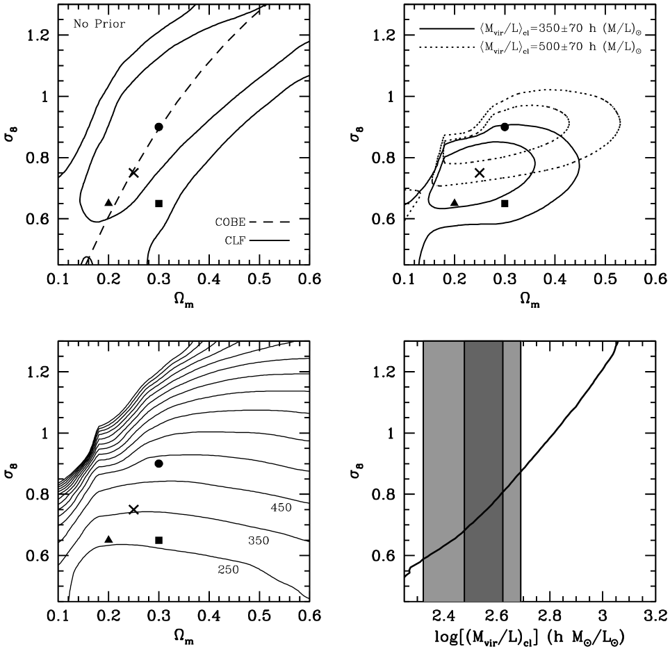
Figure 1: The upper left panel plots the 68 and 95 percent confidence levels of ${\cal L}_{\rm CLF}(\Omega_{m},\sigma_{8})$ (solid lines). For comparison, the dashed line indicates the value of $\sigma_{8}$ as function of $\Omega_{m}$ obtained from the COBE normalization for a flat $\Lambda$CDM cosmology with $\Omega_{b}h^{2}=0.02$, $h=0.7$, $n_{s}=1.0$ and $\tau=0.0$. The various symbols indicate the four models discussed in the text: ${\Lambda}30/90\,$(solid dot), ${\Lambda}30/65\,$(solid square), ${\Lambda}25/75\,$(cross) and ${\Lambda}20/65\,$(solid triangle). The solid and dotted contours in the upper right panel show the 68 and 95 percent confidence levels of ${\cal L}_{\rm CLF}(\Omega_{m},\sigma_{8})$ when combined with a Gaussian prior on the mass-to-light ratio of clusters (as indicated). The lower left panel plots contours of constant $\langle M_{\rm vir}/L\rangle_{\rm cl}$ at values of $250,350,450,...,1550h\>({\rm M}/{\rm L})_{\odot}$. For clarity, the first three contours are labelled. Finally, the lower right panel plots the value of $\sigma_{8}$ that maximizes ${\cal L}_{\rm CLF}(\Omega_{m},\sigma_{8})$ for given $\Omega_{m}$ as function of the $\langle M_{\rm vir}/L\rangle_{\rm cl}$ of the corresponding model. Clearly, higher values of $\langle M_{\rm vir}/L\rangle_{\rm cl}$ imply higher normalizations $\sigma_{8}$, as parameterized by equation (17). The light (dark) gray regions indicate the 95 (68) percent confidence levels on the observed $\langle M_{\rm vir}/L\rangle_{\rm cl}$ (see Section 2.3).

2.2 Cosmological Constraints

Both $n(M)$ and $b(M)$ are cosmology dependent. Whether or not a CLF can be found that results in good fits to the observed $\Phi(L)$ and $\xi_{\rm gg}(r,L)$ therefore depends on the cosmological model adopted, and this method may therefore be used to place constraints on cosmological parameters. In YMB03 we used data from the 2dFGRS to constrain the matter density $\Omega_{m}$ in a flat $\Lambda$CDM cosmology. We only considered cosmological models consistent with the recent weak lensing constraints of Hoekstra, Yee & Gladders (2002), i.e., $\sigma_{8}\Omega_{m}^{0.52}=0.46$, and adopted an average cluster mass-to-light ratio of $\langle M/L\rangle_{\rm cl}=500h\>({\rm M}/{\rm L})_{\odot}$. It was shown that under these conditions the best-fit model has $\Omega_{0}=0.3$ (and thus $\sigma_{8}=0.9$), in excellent agreement with the standard concordance cosmology.

Here we present a more detailed investigation. Unlike in YMB03 we consider $\sigma_{8}$ and $\Omega_{m}$ as independent model parameters and let $\langle M/L\rangle_{\rm cl}$ be a free parameter (see Appendix A). We start by considering only flat cosmologies ($\Omega_{K}=0.0$) with $\Omega_{b}h^{2}=0.02$, $h=0.7$ and $n_{s}=1.0$, and investigate how the observed $\Phi(L)$ and $\xi_{\rm gg}(r,L)$ constrain $\Omega_{m}$ and $\sigma_{8}$. In Section 3 below we relax these assumptions and perform a more detailed analysis allowing $\Omega_{b}h^{2}$, $h$, and $n_{s}$ to vary as well. For each ($\Omega_{m}$,$\sigma_{8}$) we determine the CLF that best fits the 2dFGRS luminosity function of Madgwick et al. (2002) and the amplitude of $\xi_{\rm gg}(r,L)$ at the correlation lengths $r_{0}(L)$ obtained from the 2dFGRS by Norberg et al. (2002). Note that throughout this paper all luminosities are in the photometric $b_{J}$-band (uncorrected for intrinsic absorption by dust), unless specifically stated otherwise. We parameterize $\Phi(L|M)$ using a model with 7 free parameters (see Appendix A) and use Powell’s multi-dimensional direction set method (e.g., Press et al. 1992) to find those parameters that minimize

$$\chi^{2}=\chi^{2}(\Phi)+\chi^{2}(\xi)$$ (13)

and thus maximize the likelihood ${\cal L}_{\rm CLF}\equiv{\rm e}^{-\chi^{2}/2}$. Here the first term

$$\chi^{2}(\Phi)=\sum_{i=1}^{N_{\Phi}}\left[{\Phi(L_{i})-\hat{\Phi}(L_{i})\over\Delta\hat{\Phi}(L_{i})}\right]^{2},$$ (14)

measures the goodness-of-fit to the observed LF $\hat{\Phi}(L_{i})$ with errors $\Delta\hat{\Phi}(L_{i})$. The second term is defined by

$$\chi^{2}(\xi)=\sum_{i=1}^{N_{\xi}}\left[{\xi_{\rm gg}(\hat{r}_{0}(L_{i}),L_{i})-\hat{\xi}_{\rm gg}(\hat{r}_{0}(L_{i}),L_{i})\over\Delta\hat{\xi}_{\rm gg}(\hat{r}_{0}(L_{i}),L_{i})}\right]^{2},$$ (15)

and measures the goodness-of-fit to the amplitudes of the galaxy-galaxy correlation functions. Note that we compute $\xi_{\rm gg}(r,L)$ at the observed correlation lengths $\hat{r}_{0}(L)$. These are compared to the observed values $\hat{\xi}_{\rm gg}(\hat{r}_{0}(L_{i}),L_{i})$, which by definition are equal to unity. The errors $\Delta\hat{\xi}_{\rm gg}(\hat{r}_{0}(L_{i}),L_{i})$ are computed from the errors on $\hat{r}_{0}(L_{i})$ and the power-law slope of $\hat{\xi}_{\rm gg}(r,L_{i})$ quoted by Norberg et al. (2002).

The upper left panel of Figure 1 plots the 68 and 95 percent confidence levels, obtained by integrating under the likelihood surface using the flat priors $0.1\leq\Omega_{m}\leq 0.6$ and $0.45\leq\sigma_{8}\leq 1.30$. As is apparent, the observed abundance and clustering properties constrain $\Omega_{m}$ and $\sigma_{8}$ to a fairly broad valley in $(\Omega_{m},\sigma_{8})$ parameter space, and all four cosmologies listed in Table 1 are consistent with the observations at better than 95 percent confidence. Cosmologies with small $\Omega_{m}$ and large $\sigma_{8}$ and those with large $\Omega_{m}$ and small $\sigma_{8}$ are ruled out at more than 95 percent confidence. For comparison, the dashed line indicates the relation between $\sigma_{8}$ and $\Omega_{m}$ that best-fits the COBE data (Bennett et al. 1996). This COBE constraint nicely coincides with the valley floor of ${\cal L}_{\rm CLF}(\Omega_{m},\sigma_{8})$, therewith indicating that both the CMB anisotropies and the galaxy clustering indicate the same shape of the power spectrum $P(k)$.

Understanding how $\Phi(L)$ and $\xi_{\rm gg}(r,L)$ constrain $\sigma_{8}$ and $\Omega_{m}$ is somewhat complicated. To guide the discussion, Figure 2 plots the bias, $b(M)$, and the evolved, non-linear correlation function of the dark matter $\xi_{\rm DM}(r)$ (equation [12]) for the four extreme cosmologies considered. First of all, the fact that we demand a fit to the observed LF hardly imposes any constraints at all; $\Phi(L)$ only depends on the halo mass function, and one can always choose an appropriate $\Phi(L|M)$ so that one fits $\Phi(L)$ perfectly no matter what the shape or normalization of $n(M)$. We only include the observed LF as a constraint since it sets the normalization of the CLF, which allows us to compute mass-to-light ratios. As we show below, this proves to be an important asset. The constraints on $\Omega_{m}$ and $\sigma_{8}$ are almost solely due to the constraints on $\xi_{\rm gg}(r,L)$. Typically, increasing $\sigma_{8}$ increases the amount of clustering. This is immediately apparent from Figure 2 which shows that $\xi_{\rm DM}(r)$ increases drastically from $\sigma_{8}=0.45$ to $\sigma_{8}=1.3$. Therefore, in order to keep $\xi_{\rm gg}(r,L)$ fixed at the observed values the bias $\bar{b}(L)$ needs to be lowered. This in turn requires a lower halo bias $b(M)$. However, as is apparent from equation (10), $b(M)$ can not become arbitrary small, thus imposing an upper limit on $\sigma_{8}$ for given $\Omega_{m}$. To emphasize the robustness of this result, consider the $\Omega_{m}=0.1$ and $\sigma_{8}=1.3$ cosmology. At $r=5h^{-1}\>{\rm Mpc}$, roughly the observed correlation length of galaxies with $-18\lower 3.01385pt\hbox{$\;\buildrel>\over{\sim}\;$}M_{b_{J}}-5{\rm log}h\lower 3.01385pt\hbox{$\;\buildrel>\over{\sim}\;$}-20$ (Norberg et al. 2002), the dark matter correlation function is equal to $4.4$. Using that $\xi_{g}g(r=5h^{-1}\>{\rm Mpc})\simeq 1$ implies that these galaxies require an average bias of $\bar{b}(L)\simeq 0.48$ (cf. equation [5]). This, however, is smaller than the minimum of $b(M)$ (see Figure 2). Therefore, no matter in what haloes these galaxies reside, their correlation function will always be larger than observed. This cosmology is therefore ruled out, a result that is robust against whatever we assume regarding the CLF.

To understand why cosmologies with both high $\Omega_{m}$ and low $\sigma_{8}$ are ruled inconsistent is less trivial. Consider, for example, the cosmology with $\Omega_{m}=0.6$ and $\sigma_{8}=0.45$. To explain the galaxy-galaxy correlation lengths obtained by Norberg et al. (2002), which range from $4.4h^{-1}\>{\rm Mpc}$ to $8.5h^{-1}\>{\rm Mpc}$, requires values for $\bar{b}(L)$ in the range $1.7$ to $3.2$. As is apparent from equation 5 and the left panel of Figure 2, this can be accomplished by, for example, distributing all galaxies over haloes within the relatively narrow range $10^{13}h^{-1}\>{\rm M_{\odot}}\lower 3.01385pt\hbox{$\;\buildrel<\over{\sim}\;$}M\lower 3.01385pt\hbox{$\;\buildrel<\over{\sim}\;$}10^{14}h^{-1}\>{\rm M_{\odot}}$. Therefore, in principle, one should be able to find a halo occupation model for this cosmology that is perfectly consistent with the data. The fact that our model can not accurately match the data must therefore reflect a restriction due to the parameterization of the CLF. Although our parameterization has partial observational support, results in halo occupation statistics in good agreement with semi-analytical models, and is robust against small changes (see Appendix B for a detailed discussion), we emphasize that at least part of the constraints shown in the upper left panel of Figure 1 are due to the particular parameterization of the conditional luminosity function used. Fortunately, as we shall see below, the lower-left corner of the $(\Omega_{m},\sigma_{8})$-parameter space is anyway ruled out by CMB data, and this restriction therefore does not impact on our results.

Figure 2: The halo bias $b(M)$ (left panel) and dark matter correlation function $\xi_{\rm DM}(r)$ (right panel) for four extreme cosmologies as indicated. Note how more massive haloes are more strongly clustered, and that $b(M)$ decreases with increasing $\sigma_{8}$. This largely counter-balances the increase in the clustering strength with increasing $\sigma_{8}$, thus explaining to a large extent why the observed clustering of galaxies only puts very mild constraints on $\sigma_{8}$ (see text for a more detailed discussion).

2.3 The mass-to-light ratios of clusters

One of the 7 free parameters of our $\Phi(L|M)$ parameterization is $\langle M/L\rangle_{\rm cl}$, the average mass-to-light ratio of clusters of galaxies with $M\geq 10^{14}h^{-1}\>{\rm M_{\odot}}$ (see Appendix A). Note that the halo mass $M$ is defined as the mass within the radius inside of which the average overdensity is $180$. In order to facilitate a more direct comparison with mass-to-light ratios available in the literature we convert $M/L$ to $M_{\rm vir}/L$, where $M_{\rm vir}$ is defined as the mass within the virial radius, inside of which the average density is $\Delta_{\rm vir}$ times the critical density. We adopt

$$\Delta_{\rm vir}=18\pi^{2}+82(\Omega_{m}-1)-39(\Omega_{m}-1)^{2}$$ (16)

(Bryan & Norman 1998). To convert $M$ to $M_{\rm vir}$ we also need a model for the halo concentration as function of halo mass and cosmology, for which we use the model of Eke, Navarro & Steinmetz (2001). In what follows, whenever masses correspond to the virial mass we explicitely write $M_{\rm vir}$.

The lower left panel of Figure 1 plots contours of the best-fit value of $\langle M_{\rm vir}/L\rangle_{\rm cl}$. Typically, models with higher $\sigma_{8}$ require higher values of $\langle M_{\rm vir}/L\rangle_{\rm cl}$ in order to fit the observed abundances and clustering properties of galaxies. This is easy to understand; consider once again the $\Omega_{m}=0.1$ and $\sigma_{8}=1.3$ cosmology. As discussed in the previous section, this cosmology is ruled out because the dark matter is too strongly correlated; there are simply no haloes with sufficiently small bias, $b(M)$, such that the galaxy-galaxy correlation function can be made consistent with observations. The discrepancy with the data is minimized when all galaxies reside in haloes with $M\simeq 10^{10}h^{-1}\>{\rm M_{\odot}}$, for which $b(M)$ is mimimal. Clearly, galaxies need to avoid more massive haloes since otherwise they would overpredict the galaxy-galaxy correlation strength even more. This ‘avoidance’ of massive haloes explains the extremely large mass-to-light ratio of clusters for this cosmology (see lower left panel of Figure 1). If $\sigma_{8}$ is lowered, the dark matter becomes less strongly clustered. Slowly, galaxies are required to populate more and more massive haloes in order to match the observed correlation lengths. This implies that $\langle M_{\rm vir}/L\rangle_{\rm cl}$ has to decrease. In addition, lowering $\sigma_{8}$ strongly decreases the abundance of massive haloes. Since the abundance of galaxies is fixed by the observed LF, one expects, on average, more galaxies per halo. This again will cause $M/L$ to decrease with decreasing $\sigma_{8}$. This example shows how constraints on the abundance and clustering properties of galaxies yields a cluster mass-to-light ratio that depends strongly on both $\Omega_{m}$ and $\sigma_{8}$.

It is apparent from Figure 1 that $\langle M_{\rm vir}/L\rangle_{\rm cl}$ varies strongly with position along contours of constant ${\cal L}_{\rm CLF}$. This indicates that we can significantly tighten the constraints on $\Omega_{m}$ and $\sigma_{8}$ by using additional constraints on $\langle M_{\rm vir}/L\rangle_{\rm cl}$. Using a variety of techniques to measure cluster masses, Bahcall et al. (2000) obtain $\langle M_{\rm vir}/L_{B}\rangle_{\rm cl}=(330\pm 77)h\>({\rm M}/{\rm L})_{\odot}$ (where $L_{B}$ is the total $B$-band luminosity, uncorrected for internal extinction). Carlberg et al. (1996), using the CNOC Cluster Survey, obtain $\langle M_{\rm vir}/L_{B}\rangle_{\rm cl}=(363\pm 65)h\>({\rm M}/{\rm L})_{\odot}$ (where we have converted the Gunn $r$-band luminosity to $L_{B}$ using $L_{r}=1.23L_{B}$, see Bahcall & Comerford 2002). Taking the average from these two measurements we obtain $\langle M_{\rm vir}/L_{B}\rangle_{\rm cl}=(350\pm 70)h\>({\rm M}/{\rm L})_{\odot}$. Adding this as a (Gaussian) prior to the likelihood ${\cal L}_{\rm CLF}(\Omega_{m},\sigma_{8})$ yields the 68 and 95 percent confidence levels shown in the upper right panel of Figure 1 (solid lines). As expected, the prior on $\langle M_{\rm vir}/L\rangle_{\rm cl}$ drastically tightens the constraints on $\Omega_{m}$ and $\sigma_{8}$. Marginalizing over $\sigma_{8}$ and $\Omega_{m}$ we obtain $\Omega_{m}=0.23^{+0.17}_{-0.09}$ and $\sigma_{8}=0.75^{+0.14}_{-0.18}$ (both 95% CL), respectively. Whereas the ${\Lambda}30/65\,$, ${\Lambda}25/75\,$and ${\Lambda}20/65\,$cosmologies are all consistent with these constraints at better than 68 percent confidence, the standard ${\Lambda}30/90\,$cosmology is ruled out at the 99.99 percent confidence level! In fact, the latter requires a cluster mass-to-light ratio of $\sim 512h\>({\rm M}/{\rm L})_{\odot}$ (see Table 1), more than $2\sigma$ away from the observed value.

In order to quantify the dependence of $\sigma_{8}$ on $\langle M_{\rm vir}/L\rangle_{\rm cl}$ we proceed as follows. From ${\cal L}_{\rm CLF}(\Omega_{m},\sigma_{8})$ shown in the upper left panel of Figure 1, we determine the value of $\Omega_{m}$ that maximizes the likelihood for given $\sigma_{8}$. The lower right panel of Figure 1 plots $\langle M_{\rm vir}/L\rangle_{\rm cl}$ of this best-fit model as function of $\sigma_{8}$ (i.e., the relation between $\sigma_{8}$ and $\langle M_{\rm vir}/L\rangle_{\rm cl}$ along the valley floor), which is well approximated by

$$\sigma_{8}=0.73\left({\langle M_{\rm vir}/L\rangle_{\rm cl}\over 350\,h\,\>({\rm M}/{\rm L})_{\odot}}\right)^{0.5}$$ (17)

The light (dark) gray areas correspond to the 95 (68) percent confidence levels on $\langle M_{\rm vir}/L\rangle_{\rm cl}$. Note that, because contours of constant $\langle M_{\rm vir}/L\rangle_{\rm cl}$ are almost independent of $\Omega_{m}$ (except at $\Omega_{m}\lower 3.01385pt\hbox{$\;\buildrel<\over{\sim}\;$}0.20$), equation (17) is also very similar to the maximum $\sigma_{8}$ that is consistent with a given $\langle M_{\rm vir}/L\rangle_{\rm cl}$. Requiring that $\langle M_{\rm vir}/L\rangle_{\rm cl}<500h\>({\rm M}/{\rm L})_{\odot}$, for example, translates into an upper limit of $\sigma_{8}<0.87$.

Our modeling of the conditional luminosity function combined with constraints on the mass-to-light ratio of clusters has resulted in fairly stringent constraints on $\Omega_{m}$. It is interesting to compare this with an alternative method to constrain $\Omega_{m}$ from $\langle M_{\rm vir}/L\rangle_{\rm cl}$ directly. One can write

$$\Omega_{m}={\langle M_{\rm vir}/L\rangle_{\rm cl}\over\rho_{\rm crit}/\bar{\rho}_{L}}\,\bar{\cal B}_{\rm cl}$$ (18)

with $\bar{\rho}_{L}$ the average luminosity density in the Universe, $\rho_{\rm crit}=3H_{0}^{2}/8\pi G=2.78\times 10^{11}h^{2}\>{\rm M_{\odot}}\>{\rm Mpc}^{-3}$ the critical density, and $\bar{\cal B}_{\rm cl}$ the mass-to-light ratio bias of clusters of galaxies. Note that this ‘bias’ is not the same as $b$ defined in equation (2). Using $\langle M_{\rm vir}/L\rangle_{\rm cl}=(350\pm 70)h\>({\rm M}/{\rm L})_{\odot}$ and adopting $\rho_{L}=(1.82\pm 0.17)\times 10^{8}h\>{\rm L_{\odot}}\>{\rm Mpc}^{-3}$ (Norberg et al. 2002), we obtain

$$\Omega_{m}=(0.23\pm 0.09)\,\bar{\cal B}_{\rm cl}$$ (19)

which is equal to the estimate of $\Omega_{m}$ derived above if $\bar{\cal B}_{\rm cl}=1.0$. Remarkably enough this is also the value for $\bar{\cal B}_{\rm cl}$ suggested by observations, which indicate that $M/L$ increases as a function of scale up to $\sim 1h^{-1}\>{\rm Mpc}$, but then flattens out and remains approximately constant (Bahcall, Lubin & Dorman 1995; Bahcall et al. 2000).

2.4 Peculiar velocities

The galaxy-galaxy correlation function $\xi_{\rm gg}(r)$ used above is derived from the two-dimensional two-point correlation function $\xi(\sigma,\pi)$, which measures the excess probability over random of finding a pair of galaxies with a separation in the plane of the sky $\sigma$ and a line-of-sight separation $\pi$. Two peculiar velocity effects distort this redshift space correlation function with respect to the real space correlation function $\xi(r)$ and cause $\xi(\sigma,\pi)$ to be anisotropic. On small scales the virialized motion of galaxies within dark matter haloes cause the correlation function to be extended in the $\pi$ direction (the so called “finger-of-God” effect), while on larger scales $\xi(\sigma,\pi)$ is flattened in the $\pi$ direction due to coherent infall of galaxies onto mass concentrations (Kaiser 1987). The amplitude of this Kaiser effect depends on the matter density $\Omega_{m}$ and on the biasing of the galaxy distribution. Although the galaxy bias is a complicated function of radial scale, galaxy luminosity, and even galaxy type (Kauffmann et al. 1997; Jing et al. 1998; YMB03; BYM03), on sufficiently large scales the radial dependence should vanish (i.e., the bias $b$ is linear) and the flattening of $\xi(\sigma,\pi)$ depends on the parameter

$$\beta=\Omega_{m}^{0.6}/b.$$ (20)

Using data from the 2dFGRS, Hawkins et al. (2002) recently used a multi-parameter fit to $\xi(\sigma,\pi)$ to obtain $\beta=0.49\pm 0.09$ (68% CL), the most accurate measurement to date (cf., Hamilton, Tegmark & Padmanabhan 2000; Taylor et al. 2001; Outram, Hoyle & Shanks 2001). As outlined in Hawkins et al. (2002), the mean redshift and luminosity of the galaxies on which this measure is based are $\bar{z}=0.15$ and $1.4$ times the characteristic luminosity $L^{*}$, respectively.

Figure 3: The left panel plots contours of constant $\beta$ computed from the CLF that maximizes ${\cal L}_{\rm CLF}$ for the given $\Omega_{m}$ and $\sigma_{8}$. The contours shown correspond to (from top to bottom) $\beta=0.67,0.58,0.40,0.31$ which are the 68 and 95 percent confidence levels of $\beta$ as obtained by Hawkins et al. (2002) from the 2dFGRS. The right panel plots the 68 and 95 percent confidence levels of ${\cal L}_{\rm CLF}(\Omega_{m},\sigma_{8})$ obtained using the priors as indicated. Here $G(\beta)$ refers to the Gaussian prior $\beta=0.49\pm 0.09$, while $G(\beta,\Upsilon)$ refers to the combined prior of $G(\beta)$ plus $\langle M_{\rm vir}/L\rangle_{\rm cl}=(350\pm 70)h\>({\rm M}/{\rm L})_{\odot}$.

The problem with interpreting constraints on $\beta$ in terms of constraints on the matter density $\Omega_{m}$ is that the bias parameter $b$ is notoriously hard to measure. However, it can be computed straightforwardly from the CLF, and as a function of galaxy luminosity. For each of the ($\Omega_{m},\sigma_{8}$)-models we compute $\bar{b}(1.4L^{*})$ from the best-fit CLF using equation (6). We convert this bias and $\Omega_{m}$ to their corresponding values at $\bar{z}=0.15$ using the method outlined in BYM03 and compute the likelihood ${\cal L}_{\beta}$ that the value of $\beta$ found by Hawkins et al. (2002) originates from the given cosmology. The contours in the left panel of Figure 3 indicate the corresponding 68 and 95 percent confidence levels. As is apparent, constraints on $\beta$ only yield highly degenerate constraints on $\Omega_{m}$ and $\sigma_{8}$. Note, however, that contours of constant ${\cal L}_{\beta}$ run almost perpendicular to those of constant ${\cal L}_{\rm CLF}$ (cf., upper left panel of Figure 1). This indicates that $\beta$ and $\xi_{\rm gg}(r,L)$, although both obtained from $\xi(\sigma,\pi)$, constrain $\Omega_{m}$ and $\sigma_{8}$ in different ways. Using $\beta=0.49\pm 0.09$ as a Gaussian prior on ${\cal L}_{\rm CLF}(\Omega_{m},\sigma_{8})$, results in the 68 and 95 percent confidence levels shown in the right panel of Figure 3 (solid contours). Both $\Omega_{m}$ and $\sigma_{8}$ are now well constraint; marginalizing over $\sigma_{8}$ and $\Omega_{m}$ we obtain $\Omega_{m}=0.27^{+0.16}_{-0.12}$ and $\sigma_{8}=0.87^{+0.22}_{-0.26}$ (both 95% CL), respectively. Note that these constraints on $\Omega_{m}$ and $\sigma_{8}$ are obtained from the 2dFGRS alone, independent of any other data set.

Hawkins et al. (2002) combined their constraint on $\beta$ with a determination of the bias obtained by Verde et al. (2002) from an analysis of the 2dFGRS bispectrum. This yielded $\Omega_{m}=0.23\pm 0.09$, consistent with the results presented here at the $1\sigma$ level. It is extremely reassuring that two wildly different methods (CLF modeling versus bispectrum analysis) yield values for the bias in such good agreement.

Finally, upon combining the priors on $\beta$ and $\langle M_{\rm vir}/L\rangle_{\rm cl}$ we obtain the 68 and 95 percent contour levels indicated by dotted contours. Marginalizing over $\sigma_{8}$ and $\Omega_{m}$ we obtain $\Omega_{m}=0.27^{+0.14}_{-0.10}$ and $\sigma_{8}=0.77^{+0.10}_{-0.14}$ (both 95% CL), respectively. Whereas the constraint on $\Omega_{m}$ is perfectly consistent with the concordance value, the constraint on the cluster mass-to-light ratios strongly favors low-$\sigma_{8}$ models over the standard $\sigma_{8}=0.9$. Keep in mind, however, that this analysis is restricted to flat $\Lambda$CDM cosmologies with $\Omega_{b}h^{2}=0.02$, $h=0.7$, and $n_{s}=1.0$. In what follows we relax these constraints and perform a more detailed analysis including additional data on CMB anisotropies.

3 A joint CMB plus LSS analysis

3.1 Cosmic Microwave Background

Undoubtedly the most stringent constraints on cosmological parameters come from measurements of the angular CMB temperature power spectrum. Results from COBE (Bennett et al. 1996), BOOMERANG (Netterfield et al. 2002), MAXIMA (Hanany et al. 2000), DASI (Halverson et al. 2002), VSA (Scott et al. 2002), CBI (Pearson et al. 2002) and WMAP (Bennett et al. 2003) have combined to produce a power spectrum of CMB temperature anisotropies with the first three acoustic peaks resolved. This has resulted in stringent constraints on cosmological parameters (e.g., Wang, Tegmark & Zaldarriaga 2002; de Bernardis et al. 2002; Pryke et al. 2002; Sievers et al. 2002; Efstathiou et al. 2002; Spergel et al. 2003). Unfortunately, because of the unknown amount of Thompson scattering experienced by CMB photons, these data only put constraints on the combination $\sigma_{8}{\rm e}^{-\tau}$. Here $\tau$ is the optical depth for Thompson scattering, which depends, amongst others, on the reionization redshift $z_{\rm re}$. The absence of a clear Gunn-Peterson trough in the spectra of high-redshift quasars puts a lower limit on the reionization epoch of $z_{\rm re}\lower 3.01385pt\hbox{$\;\buildrel>\over{\sim}\;$}5.5$ (e.g., Becker et al. 2001; Fan et al. 2001), and therewith on $\tau$. In addition, the observed height of the first acoustic peak requires $\tau\lower 3.01385pt\hbox{$\;\buildrel<\over{\sim}\;$}0.4$ (e.g., Griffiths, Barbosa & Liddle 1999; Ruhl et al. 2002). Because of these limits on $\tau$ the uncertainty on $\sigma_{8}$ is limited to about 30 percent.

To illustrate the constraints that pre-WMAP CMB data put on ($\Omega_{m}$,$\sigma_{8}$)-parameter space we use the Monte-Carlo Markov (MCM) chains of Lewis & Bridle (2002; hereafter LB02). These consist of large numbers of cosmological models, each of which is characterized by $N$ model parameters. The chains are constructed using the Metropolis-Hastings algorithm, which ensures that the number density distribution of these models in the $N$-dimensional parameter space traces out the posterior probability distribution that the observed data originates from the given cosmology (see LB02 and references therein). The clear advantage of this MCM chain technique is that it samples the entire $N$-dimensional posterior giving far more information than just the marginalized distributions of each of the $N$ individual parameters (which is what is commonly presented). In addition, it is straightforward to extract the marginalized distribution in any sub-dimensional parameter space by simple projection.

Here we use the publicly available $N=6$ Markov Chain of LB02 consisting of $\sim 11500$ weakly correlated cosmological models. The six parameters that label each model are: $\Omega_{b}h^{2}$, $\Omega_{c}h^{2}$, $h$, $n_{s}$, the redshift $z_{\rm re}$ at which the reionization fraction is a half, and $A_{s}$, a measure for the amplitude of the initial power spectrum. Most of these parameters have weak, flat priors (see LB02 for details), except for the Hubble parameter which has a Gaussian prior of $h=0.72\pm 0.08$ (taken from the HST key project, Freedman et al. 2001). All models are computed assuming purely adiabatic, scalar-only, Gaussian primordial perturbations, $\Omega_{K}=0$, non-interacting CDM, and an effective equation of state for the dark energy $w=-1$ (corresponding to a pure cosmological constant). The data used to construct the chains consists of a combination of the results of COBE, BOOMERANG, MAXIMA, DASI, VSA, and CBI in the form of band power estimates for the temperature CMB power spectrum. The CBI data with $l>2000$, which is most likely due to non-linear effects, is ignored.

Figure 4 plots the distribution of models of the MCM chain in the ($\Omega_{m}$, $\sigma_{8}$) parameter space, gray-scale coded according to their value of $h$ (left panel) or $\tau$ (right panel). As mentioned above, the number density distribution of models is directly proportional to the marginalized likelihood ${\cal L}_{\rm CMB}(\Omega_{m},\sigma_{8})$. The two contours indicate the 68 and 95 percent confidence levels, obtained by integrating under the likelihood surface. Marginalizing over $\sigma_{8}$ and $\Omega_{m}$ we obtain $\Omega_{m}=0.26^{+0.22}_{-0.12}$ and $\sigma_{8}=0.80^{+0.19}_{-0.18}$ (95% CL), respectively. The 95 percent confidence interval for $\sigma_{8}$ therefore covers the entire range of values for $\sigma_{8}$ quoted in the literature. As apparent from the gray-scale coding in the panel on the right, this uncertainty on $\sigma_{8}$ is due to the $\sigma_{8}$–${\rm e}^{-\tau}$ degeneracy mentioned above. Higher values of $\sigma_{8}$ (for given $\Omega_{m}$) correspond to higher optical depth, and therefore to a higher redshift of reionization. The constraints on $\Omega_{m}$ are almost entirely due to the Gaussian prior on $h$, as is immediately evident from the gray-scale coding in the left panel. Whereas the CMB data alone mainly constrains $\Omega_{K}$ (through the location of the first acoustic peak), the combination of CMB data plus a prior on the Hubble constant already puts useful constraints on $\Omega_{m}$ (e.g., Rubiño-Martin et al. 2002; LB02).

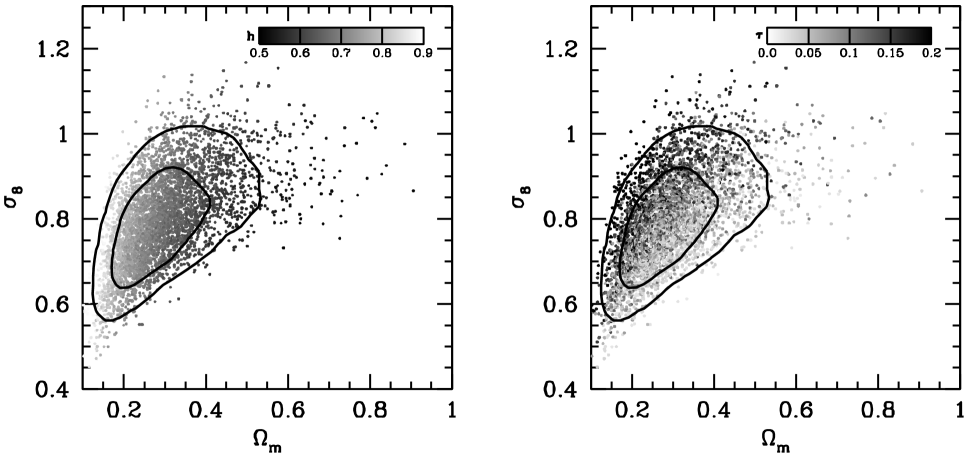
Figure 4: The points correspond to cosmological models from the Monte-Carlo Markov chain of LB02, and are gray-scale coded according to their values for $h$ (left panel) and $\tau$ (right panel). The chain is constructed such that the number density of points is proportional to the marginalized likelihood ${\cal L}_{\rm CMB}(\Omega_{m},\sigma_{8})$ with the 68 and 95 percent confidence levels indicates with contours. See text for details.

3.2 Combining CMB plus 2dFGRS

An extremely attractive feature of the MCM chains is that it is straightforward to compute likelihoods including additional data. The weight of each model is simply adjusted proportional to the likelihood under the new constraint, a technique known as importance sampling (see LB02 for details). The new, marginalized likelihood is subsequently obtained from the weighted number density of points as a function of $\Omega_{m}$ and $\sigma_{8}$. Using importance sampling we compute the combined likelihood ${\cal L}_{\rm tot}$ that both the CMB data plus the $\Phi(L)$ and $\xi_{\rm gg}(r,L)$ originate from the given cosmology.

The 68 and 95 percent confidence levels of ${\cal L}_{\rm tot}(\Omega_{m},\sigma_{8})$ are shown in the upper left panel of Figure 5 (solid lines). As is apparent from a comparison with the likelihood from the CMB data alone (dotted contours), the LSS data adds virtually no new constraints. In other words, any model (in the 6-dimensional parameter space studied here) that fits the CMB data also fits the galaxy correlation lengths as function of luminosity. Although the lack of improvement on the constraints is perhaps somewhat disappointing, it is a beautiful demonstration of the level of concordance among two completely independent sets of data.

As in Section 2 above we can tighten the constraints on $\Omega_{m}$ and $\sigma_{8}$ by using priors on the cluster mass-to-light ratio and/or $\beta$. Including the Gaussian prior $\langle M_{\rm vir}/L\rangle_{\rm cl}=(350\pm 70)h\>({\rm M}/{\rm L})_{\odot}$ results in the 68 and 95 percent confidence levels shown in the upper right panel. Clearly, the constraints on $\langle M_{\rm vir}/L\rangle_{\rm cl}$ restrict both $\Omega_{m}$ and $\sigma_{m}$ to relatively low values (compared to the parameter space allowed by the CMB data). Marginalizing over $\sigma_{8}$ and $\Omega_{m}$ we obtain $\Omega_{m}=0.25^{+0.09}_{-0.08}$ and $\sigma_{8}=0.76^{+0.14}_{-0.12}$ (both 95% CL), respectively. This is inconsistent with the standard $\sigma_{8}=0.9$ at $\sim 2\sigma$. Fairly similar results are obtained if instead of the prior on $\langle M_{\rm vir}/L\rangle_{\rm cl}$ we include the Gaussian prior $\beta=0.49\pm 0.09$ ($\Omega_{m}=0.26^{+0.15}_{-0.09}$, $\sigma_{8}=0.80^{+0.15}_{-0.14}$, see lower left panel of Figure 5). Finally, upon including both priors we obtain the confidence levels shown in the lower right panel with marginalized probability distributions $\Omega_{m}=0.25^{+0.10}_{-0.07}$ and $\sigma_{8}=0.78\pm 0.12$ (both 95% CL).

Figure 5: The dotted contours in each of the four panels indicate the 68 and 95 percent confidence levels on $\Omega_{m}$ and $\sigma_{8}$ as determined from the CMB data plus the Gaussian prior $G(h)$ on the Hubble parameter: $h=0.72\pm 0.08$. The solid contours indicate the same confidence levels of the combined likelihood ${\cal L}_{\rm tot}$ with the priors as indicated, using the same nomenclature as in Figure 3.

In summary, the observed clustering properties of galaxies are in perfect agreement with matter power spectra that fit the current CMB data. The conditional luminosity function models presented here allow us to compute mass-to-light ratios and galaxy bias in a completely self-consistent way, which in turn allows us to significantly tighten the constraints on $\Omega_{m}$ and $\sigma_{8}$. The strongest constraints come from the observed mass-to-light ratio of clusters, which strongly argues for cosmologies with both $\Omega_{m}$ and $\sigma_{8}$ reduced by $\sim 15$ percent with respect to the standard values of $0.3$ and $0.9$, respectively.

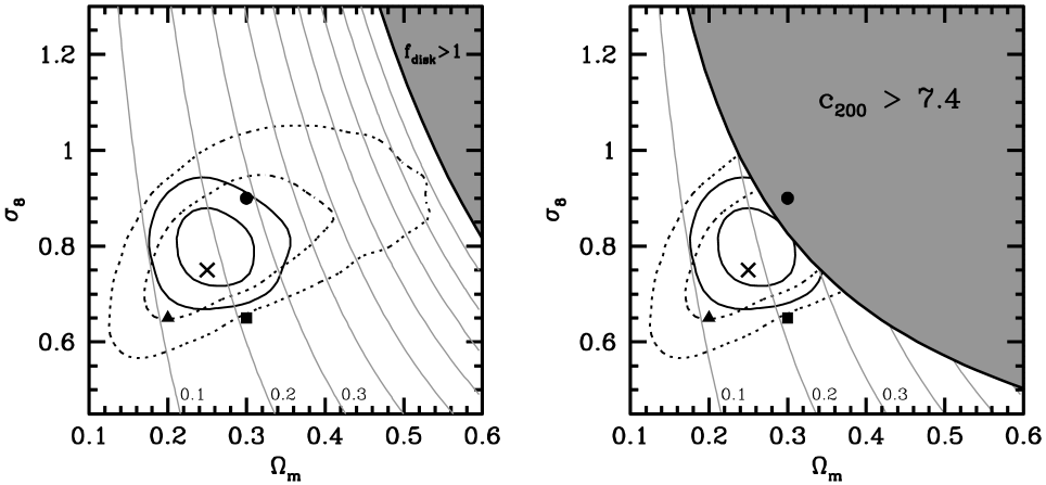
Figure 6: Thin gray lines in both panels indicate contours of constant $f_{\rm disk}$ (equation [25]). The contours corresponding to $f_{\rm disk}=0.1$, $0.2$, and $0.3$ are labelled for clarity. The gray areas correspond to $f_{\rm disk}>1$ (left panel) and $c_{200}>7.4$ (right panel), and indicate the regions of parameter space that are excluded according to the observed baryonic Tully-Fisher relation and the observed rotation curves of LSB galaxies, respectively (see text for details). The dotted contours in both panels correspond to the 68 and 95 percent confidence levels of ${\cal L}_{\rm CMB}(\Omega_{m},\sigma_{8})$ (cf. Figures 4 and 5), while the solid contours indicate the same levels of confidence but for ${\cal L}_{\rm tot}(\Omega_{m},\sigma_{8})$ with the Gaussian priors $\langle M_{\rm vir}/L\rangle_{\rm cl}=(350\pm 70)h\>({\rm M}/{\rm L})_{\odot}$ and $\beta=0.49\pm 0.09$ (cf. lower right panel of Figure 5). The symbols are as in Figure 1 and correspond to the four models in Table 1.

4 Implications

As outlined in Section 1, despite the large uncertainty in $\sigma_{8}$, most numerical simulations of structure formation in a $\Lambda$CDM cosmology have adopted $\Omega_{m}=0.3$ and $\sigma_{8}=0.9$. This has also been the preferred cosmology for studies of galaxy formation. Yet, several studies over the past years, including this one, have suggested values for $\Omega_{m}$ and/or $\sigma_{8}$ that are reduced with respect to these standard values.

In this section we investigate the implications that small modifications of $\sigma_{8}$ and $\Omega_{m}$ have on the structure and formation of galaxies and their associated CDM haloes. In particular, we focus on two problems that have been identified in recent years for the standard $\Lambda$CDM cosmology; the problem of matching the TF zero-point and the inconsistencies between observed and predicted rotation curves for dwarf and low surface brightness galaxies.

4.1 The Baryonic Tully-Fisher Relation

Disk galaxies follow a scaling relation between luminosity and rotation velocity known as the Tully-Fisher (TF) relation. Since the rotation velocity is a dynamical mass measure, the zero-point of the Tully-Fisher relation sets a characteristic mass-to-light ratio and can therefore, in principle, be used to constrain cosmological parameters (see e.g., van den Bosch 2000). Here we focus on the so-called “baryonic” Tully-Fisher relation between disk mass and rotation velocity (McGaugh et al. 2000; Bell & de Jong 2001). Observationally, the disk mass is obtained by multiplying the disk luminosity with the stellar mass-to-light ratio and adding the contribution of the cold gas in the disk. Here we use the results of McGaugh et al. (2000), who found

$$M_{\rm disk}=1.97\times 10^{9}h^{-2}\>{\rm M_{\odot}}\,\left({V_{\rm rot}\over 100\>{\rm km}\,{\rm s}^{-1}}\right)^{4}$$ (21)

Defining dark matter haloes as spheres with an average density inside the virial radius, $r_{\rm vir}$, that is $\Delta_{\rm vir}$ times the critical density $\rho_{\rm crit}$, one obtains the following relation between the virial mass $M_{\rm vir}$ and the circular velocity $V_{\rm vir}$ at the virial radius:

$$M_{\rm vir}=2.33\times 10^{11}h^{-1}\>{\rm M_{\odot}}\left({V_{\rm vir}\over 100\>{\rm km}\,{\rm s}^{-1}}\right)^{3}\,\left({\Delta_{\rm vir}\over 200}\right)^{-1/2}$$ (22)

The cosmology dependence enters through $\Delta_{\rm vir}$ (eq. [16]). The mass of a disk galaxy that forms inside this halo can be expressed as

$$M_{\rm disk}=f_{\rm disk}\,\left({\Omega_{b}\over\Omega_{m}}\right)\,M_{\rm vir}$$ (23)

Here $f_{\rm disk}$ is the fraction of baryonic material in the halo that ends up in the disk. Equating (23) to the observed baryonic TF relation (21) yields

$$f_{\rm disk} = 0.423\,h\,\Omega_{m}\,\left({\Omega_{b}h^{2}\over 0.02}\right)^{-1}\,\left({V_{\rm rot}\over V_{\rm vir}}\right)^{4}\times$$ (24)

$$\left({\Delta_{\rm vir}\over 200}\right)^{1/2}\left({V_{\rm vir}\over 100\>{\rm km}\,{\rm s}^{-1}}\right)$$

This fraction has to obey $f_{\rm disk}\leq 1$, at least under the standard assumption that the baryonic fraction inside dark matter haloes can not exceed the universal value. The strongest constraint on cosmological parameters comes from the high-$V_{\rm vir}$ end. Using (22) and evaluating $f_{\rm disk}$ at $M_{\rm vir}=3\times 10^{12}h^{-1}\>{\rm M_{\odot}}$, which is roughly the maximum halo mass for disk galaxies, one obtains

$$f_{\rm disk}=0.991\,h\Omega_{m}\,\left({\Omega_{b}h^{2}\over 0.02}\right)^{-1}\,\left({V_{\rm rot}\over V_{\rm vir}}\right)^{4}\,\left({\Delta_{\rm vir}\over 200}\right)^{2/3}$$ (25)

This fraction depends strongly on the ratio of the observed rotation velocity to the circular velocity of the halo. In the CDM paradigm dark matter haloes follow the universal NFW density distribution

$$\rho(r)={\bar{\delta}\,\bar{\rho}\over(r/r_{s})(1+r/r_{s})}$$ (26)

(Navarro, Frenk & White 1997). Here $r_{s}$ is a characteristic radius, $\bar{\rho}=\Omega_{m}\rho_{\rm crit}$ is the average density of the Universe, and $\bar{\delta}$ is a dimensionless amplitude which can be expressed in terms of the halo concentration parameter $c\equiv r_{\rm vir}/r_{s}$ as

$$\bar{\delta}={\Delta_{\rm vir}\over 3}\,{c^{3}\over{\rm ln}(1+c)-c/(1+c)}$$ (27)

The circular velocity curve of a NFW density distribution reaches a maximum $V_{\rm max}$ at a radius $r=2.163r_{s}$. The ratio of $V_{\rm max}$ to the virial velocity is given by

$${V_{\rm max}\over V_{\rm vir}}=0.465\,\sqrt{c\over{\rm ln}(1+c)-c/(1+c)}$$ (28)

and is typically larger than unity. We use the model of Eke, Navarro & Steinmetz (2001) to compute $c$ as function of halo mass and cosmology, and we assume that $V_{\rm rot}=V_{\rm max}$, i.e., that the observed, flat part of the rotation curve coincides with $V_{\rm max}$. Detailed models (Mo, Mao & White 1998; van den Bosch 2001; 2002) indicate that in cases were $f_{\rm disk}$ is sufficiently large $V_{\rm rot}>V_{\rm max}$ due to the contribution of the disk to the circular velocity. We ignore this effect for the moment, but caution that the $f_{\rm disk}$ thus derived may be an underestimate.

In Figure 6 we plot contours of constant $f_{\rm disk}$ as function of $\Omega_{m}$ and $\sigma_{8}$. The gray region in the left panel indicates the cosmologies for which $f_{\rm disk}>1$ and which are thus excluded. In addition, we plot the 68 and 95 percent confidence levels of ${\cal L}_{\rm CMB}$ (dotted contours) and of ${\cal L}_{\rm tot}$ plus priors on $\langle M_{\rm vir}/L\rangle_{\rm cl}$ and $\beta$ (solid contours). The constraint from the TF zero-point ($f_{\rm disk}\leq 1$) only rules out models which are already inconsistent with the CMB data at more than 95 percent confidence. Typically $f_{\rm disk}$ decreases with decreasing $\Omega_{m}$ and decreasing $\sigma_{8}$. Note that for the standard $\Lambda$CDM cosmology, with $\Omega_{m}=0.3$ and $\sigma_{8}=0.9$, only about 30 percent of the available baryons in a $3\times 10^{12}h^{-1}\>{\rm M_{\odot}}$ halo should be present in the disk. In the case of cosmologies favored by the CMB plus LSS data presented here, this fraction is even lower, between 10 and 20 percent. Thus, in order to explain the zero-point of the baryonic TF relation, only a minor fraction of the baryonic mass within $r_{\rm vir}$ can become part of the disk; the remaining baryonic material either remains in the halo as hot gas, or is expelled from the halo. Note that $f_{\rm disk}$ scales with $V_{\rm vir}$ such that this fraction is even lower in lower mass haloes. This requirement for a physical mechanism that can prevent baryons from ending up in cold gas or stars is also obvious from a direct comparison of the halo mass function with the galaxy luminosity function (e.g., White & Rees 1978; White & Frenk 1991; YMB03) and remains one of the most challenging puzzles in the framework of galaxy formation.

Figure 7: Left panel: The average mass-to-light ratio as function of halo mass for the four cosmological models listed in Table 1, as obtained from the best-fit CLF. The solid dot indicates the average mass-to-light ratio of clusters $\langle M_{\rm vir}/L\rangle_{\rm cl}=350\pm 70h\>({\rm M}/{\rm L})_{\odot}$, where the errorbars indicate the $1\sigma$ interval. Right panel: Tully-Fisher relations for the four cosmologies listed in Table 1, obtained from the $\langle M_{\rm vir}/L\rangle(M)$ shown in the left panel as described in the text. For comparison, the solid dots indicate the Tully-Fisher relation for the ‘local calibrator sample’ of Tully & Pierce (2000).

4.2 The Tully-Fisher Zero-Point

Detailed semi-analytical models for the formation of galaxies have so far been unsuccessful in simultaneously fitting the galaxy LF and the TF zero-point. Initially, when these studies focussed on Einstein-de Sitter cosmologies, the discrepancies where found to be extremely large, with models tuned to fit the LF predicting much too faint luminosities for a given rotation velocity (e.g., Kauffmann, White & Guiderdoni 1993; Cole et al. 1994). Heyl et al. (1995) showed that this could be significantly improved upon by lowering $\Omega_{m}$, but the overall agreement remained unsatisfactory. Even for the currently popular $\Lambda$CDM cosmology with $\Omega_{m}=0.3$ and $\sigma_{8}=0.9$ no semi-analytical models presented to date has been able to simultaneously fit the LF and TF zero-point (Somerville & Primack 1999; Cole et al. 2000; Benson et al. 2000, 2002; Mathis et al. 2002). Remarkably enough, YMB03 found exactly the same problem when comparing the average mass-to-light ratios inferred from the CLF with those required to fit the TF zero-point. Since the CLF method makes no assumptions about how galaxies form, this indicates that the problem is not related to the (poorly understood) physics of galaxy formation, but rather is a problem of more fundamental, cosmological origin.

As shown in Section 4.1, the TF zero-point depends strongly on the concentration of dark matter haloes: more concentrated haloes have a higher $V_{\rm max}/V_{\rm vir}$, and thus a higher rotation velocity for a given disk luminosity. Since halo concentrations are strongly cosmology dependent, the TF zero-point problem outlined above may simply indicate that the standard cosmological concordance parameters are not correct. In order to access the impact of small changes in $\Omega_{m}$ and $\sigma_{8}$, consider the four cosmologies listed in Table 1. The left panel of Figure 7 plots the average mass-to-light ratios, $\langle M_{\rm vir}/L\rangle(M_{\rm vir})$, as obtained from the best-fit CLFs. The general trend is the same for all models: at $M_{\rm vir}\lower 3.01385pt\hbox{$\;\buildrel<\over{\sim}\;$}10^{11}h^{-1}\>{\rm M_{\odot}}$ the mass-to-light ratios strongly increase with decreasing halo mass. This is required in order to reconcile the faint slope of the galaxy LF with the relatively steep low-mass slope of the halo mass function (cf., YMB03). At $M_{\rm vir}\geq 10^{14}h^{-1}\>{\rm M_{\odot}}$ the mass-to-light ratio $\langle M/L\rangle$ is, by construction (see Appendix A) constant at $\langle M/L\rangle_{\rm cl}$, in good agreement with the observed flattening of mass-to-light ratios with increasing scale (Bahcall et al. 1995, 2000). Typically, lowering $\sigma_{8}$ (while keeping all other cosmological parameters fixed) reduces $\langle M/L\rangle_{\rm cl}$ and increases the mass-to-light ratios on the scales of galaxies (cf. models ${\Lambda}30/90\,$and ${\Lambda}30/65\,$). Simultaneously reducing $\sigma_{8}$ and $\Omega_{m}$ along the valley floor of ${\cal L}_{\rm CLF}$, however, leads to a reduction of $\langle M_{\rm vir}/L\rangle$ on all mass scales (cf. models ${\Lambda}30/90\,$, ${\Lambda}25/75\,$, and ${\Lambda}20/65\,$).

We can use the CLFs to compute predictions for the TF relation as follows. We assume that TF disk galaxies are the brightest galaxies in their haloes. From the CLF, it is straightforward to compute the average luminosity of the brightest galaxy, $\langle L_{c}\rangle$, as function of halo mass (see Appendix A), which we convert to magnitudes in the photometric $b_{J}$-band using $M_{\odot,b_{J}}=5.3$. Finally, the maximum rotation velocity $V_{\rm max}$ is obtained from equation (28). Assuming that these $V_{\rm max}$ are equal to the TF rotation velocities, we obtain the TF relations shown in the right panel of Figure 7. For comparison, we also plot (solid circles) the $b_{J}$ band TF relation of the ‘local calibrator sample’ of Tully & Pierce (2000). Here we have converted $B$-band magnitudes to the $b_{J}$ band using $b_{j}=B-0.28\,(B-V)$ (Blair & Gilmore 1982) and adopting $B-V=0.7$, which corresponds roughly to the average color of disk galaxies (de Jong 1996).

Compared to the data, the TF relation for the standard $\Lambda$CDM cosmology ${\Lambda}30/90\,$is somewhat too shallow, clearly underpredicting the luminosity of the more massive disk galaxies. Since the CLFs are tuned to fit the observed LF, this illustrates the TF zero-point problem outlined above. Model ${\Lambda}30/65\,$, however, predicts a somewhat steeper TF relation, in better agreement with the data, while models ${\Lambda}25/75\,$and ${\Lambda}20/65\,$predict TF zero-points that are brighter than that of model ${\Lambda}30/90\,$by as much as almost an entire magnitude. Clearly, relatively small changes in $\Omega_{m}$ and/or $\sigma_{8}$ with respect to the standard concordance values of $0.3$ and $0.9$, respectively, strongly alleviate the problem (see also Seljak 2002b,c). Although a definite answer requires a more thorough investigation, it is extremely encouraging that the same cosmological model that is preferred by the observed abundance and clustering of galaxies, predicts mass-to-light ratios on galactic scales that better match the observed TF zero-point. Remarkably enough, as shown in Section 4.1 above, this cosmology also requires lower values of $f_{\rm disk}$, and thus a stronger efficiency of preventing baryons from ending up in the disk. It remains to be seen whether detailed models for galaxy formation, can simultaneously match the LF and the TF zero-point when considering cosmologies such as ${\Lambda}25/75\,$.

4.3 Rotation Curves

In the past years numerous authors have pointed out that the rotation curves of dwarf and low-surface brightness (LSB) galaxies indicate dark matter haloes that are less centrally concentrated than predicted by the standard $\Lambda$CDM cosmology with $\sigma_{8}=0.9$ (e.g., Moore 1994; Burkert 1995; van den Bosch et al. 2000; Borriello & Salucci 2001; Blais-Ouelette, Amram & Carignan 2001; de Blok, McGaugh & Rubin 2001; de Blok & Bosma 2002; Swaters et al. 2003).

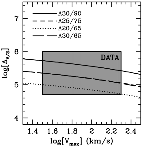
Figure 8: The concentration of dark matter haloes, expressed through the dimensionless quantity $\Delta_{V/2}$ (equation [31]) as function of the maximum circular velocity of the halo. Predictions are shown for the four cosmological models listed in Table 1 as indicated, and are computed using the Eke et al. (2001) model for halo concentrations. The gray area labelled ‘DATA’ indicates the region occupied by observed galaxies (see Alam et al. 2002). Reducing $\Omega_{m}$ and/or $\sigma_{8}$ reduces halo concentrations and thus $\Delta_{V/2}(V_{\rm max})$. Note that the $\Delta_{V/2}(V_{\rm max})$ of cosmologies ${\Lambda}30/65\,$and ${\Lambda}25/75\,$almost exactly overlap.

Since the average concentration of a halo of given mass is cosmology dependent, a constraint on halo concentrations translates into one on cosmological parameters. This principle was recently used by McGaugh, Barker & de Blok (2003). Using the high resolution hybrid H$\alpha$-HI rotation curves of LSB galaxies presented by de Blok, McGaugh & Rubin (2001) and de Blok & Bosma (2002) they derived an upper limit for the mean observed halo concentration of $c_{200}<7.4$. Here $c_{200}=r_{200}/r_{s}$ with $r_{200}$ the radius inside of which the average density of the halo is $200$ times the critical density. Using the model outlined in Navarro et al. (1997) to compute $c_{200}$ for given cosmology and halo mass McGaugh et al. (2003) obtain that

$$\sigma_{8}\Gamma_{0.6}<0.23$$ (29)

with

$$\Gamma_{0.6}=\Omega_{m}^{0.6}\,h\,{\rm exp}(-\Omega_{b}-\sqrt{2h}\Omega_{b}/\Omega_{m})-0.32\,(n_{s}^{-1}-1)$$ (30)

This is based on the assumption that all LSB galaxies reside in dark matter haloes with $M_{200}=10^{12}h^{-1}\>{\rm M_{\odot}}$. Since in general one expects that $M_{200}$ is smaller than this, and since $c$ decreases with increasing halo mass, this is a conservative upper limit.

The gray region in the upper right panel of Figure 6 indicates the part of ($\Omega_{m}$, $\sigma_{8}$) parameter space for which haloes with $M_{200}=10^{12}h^{-1}\>{\rm M_{\odot}}$ have concentrations $c_{200}>7.4$. Here we have adopted $\Omega_{b}h^{2}=0.02$, $h=0.7$, and $n_{s}=1.0$. As is apparent, the constraint (29) puts stringent constraints on $\Omega_{m}$ and $\sigma_{8}$. In fact, if taken at face value, a large fraction of the cosmologies that are consistent with the CMB data at the 95 percent confidence level or better is ruled out, including the standard $\Lambda$CDM cosmology ${\Lambda}30/90\,$. However, virtually the entire 68 percent confidence region obtained from the joined CMB plus LSS analysis presented in Section 3 above is consistent with (29). Thus, as with the TF zero-point, the problem with the observed rotation curves of dwarf and LSB galaxies may simply be alleviated by adopting a cosmology with somewhat lower $\sigma_{8}$ and/or $\Omega_{m}$ (see also Zentner & Bullock 2002).

Unfortunately, the robustness of this result is questionable for several reasons. First of all, we have adopted a halo mass of $M_{200}=10^{12}h^{-1}\>{\rm M_{\odot}}$, whereas in reality LSB galaxies will reside in haloes with a variety of halo masses. Secondly, in order to obtain a measure of $c$ from an observed rotation curve one generally fits a mass model to the data. In some cases, however, no good fit can be obtained for any value of $c$. This is often interpreted as indicating that dark matter haloes do not follow an NFW profile (i.e., the dark matter is not cold and collisionless), but may also indicate non-circular motions or other distortions (see e.g., Salucci 2001; Swaters et al. 2003).

A more robust comparison of models with data was suggested by Alam, Bullock & Weinberg (2002). Rather than using the halo concentration parameter $c$, which is difficult to extract from an observed rotation curve, Alam et al. (2002) introduced the dimensionless quantity

$$\Delta_{V/2}={\bar{\rho}(R_{V/2})\over\rho_{\rm crit}}={1\over 2}\left({V_{\rm max}\over H_{0}R_{V/2}}\right)^{2}$$ (31)

as a more robust measure of the concentration of dark matter haloes. Here $R_{V/2}$ is defined as the radius at which the rotation curve falls to half of its maximum value $V_{\rm max}$, and $\Delta_{V/2}$ thus measures the mean dark matter density inside $R_{V/2}$ in units of the critical density $\rho_{\rm crit}$. Unlike $c$ and $V_{\rm vir}$, the parameters $\Delta_{V/2}$ and $V_{\rm max}$ are easy to obtain from an observed rotation curve, without having to resort to mass model fitting. Under the assumption that the observed rotation curve is dominated by the contribution of the dark matter, a valid assumption in the case of LSB galaxies, $V_{\rm max}$ and $R_{V/2}$ can be converted directly to $c$ and $V_{\rm vir}$ and thus be compared to cosmology dependent predictions.

For the four cosmologies listed in Table 1 we compute $\Delta_{V/2}$ as function of $V_{\rm max}$ as follows. We assume that CDM haloes have a NFW density distribution and that halo concentrations depend on halo mass and cosmology according to the model of Eke et al. (2001). $V_{\rm max}$ then follows from equation (28), while $\Delta_{V/2}$ is related to the concentration parameter $c$ as

$$\Delta_{V/2}=3.36\,\Delta_{\rm vir}\,{c^{3}\over{\rm ln}(1+c)-c/(1+c)}$$ (32)

Results are shown in Figure 8. The gray area labelled ‘DATA’ indicates the region occupied by observed galaxies (see Alam et al. 2002). Models ${\Lambda}30/65\,$, ${\Lambda}25/75\,$, and ${\Lambda}20/65\,$predict halo densities inside $R_{V/2}$ that are a factor 2, 2, and 4 smaller, respectively, than for the standard concordance model ${\Lambda}30/90\,$. A reduction in $\Omega_{m}$ and/or $\sigma_{8}$ with respect to the standard concordance values thus strongly alleviates the rotation curve problem. Note that the spread in the data is larger than the difference between the four cosmologies. However, keep in mind that the model calculations reflect the average $\Delta_{V/2}$ as function of $V_{\rm max}$. Furthermore, any contribution of the baryons to $V_{\rm max}$ (ignored here) may boost $\Delta_{V/2}(V_{\rm max})$ of the data with respect to the pure dark halo models, and the curves shown here should thus be interpreted roughly as lower limits. In addition, we point out that the $\Delta_{V/2}(V_{\rm max})$ shown here is lower than the $\Delta_{V/2}(V_{\rm max})$ presented in Alam et al. (2002) for the same cosmology, especially at small $V_{\rm max}$. This is due to the different models used to compute halo concentrations: whereas we rely on the Eke et al. (2001) model, Alam et al. (2002) use the model suggested by Bullock et al. (2001) which predicts somewhat higher concentrations. These differences indicate the theoretical uncertainty regarding the concentrations of relatively low mass haloes. Although accurate constraints on cosmological parameters are therefore not possible, the general trend is clear: decreasing $\Omega_{m}$ and/or $\sigma_{8}$ reduces the concentrations of dark matter haloes, bringing them in better agreement with the data compared to the standard model with $\Omega_{m}=0.3$ and $\sigma_{8}=0.9$.

5 Summary

One of the main goals in modern cosmology is to determine the initial conditions for structure formation in the early Universe, expressed through the initial mass power spectrum $P(k)$. In this paper we assumed that $P(k)$ is a simple power-law and used data on the abundance and clustering of galaxies to constrain the normalization $\sigma_{8}$.

Because of the unknown bias of galaxies with respect to the mass distribution, previous attempts to constrain cosmological parameters from large scale structure (LSS) data have mainly focussed on the shape of $P(k)$ rather than the normalization. In this paper we analyzed data from the 2dFGRS using a technique based on the conditional luminosity function (introduced by YMB03 and BYM03) that self-consistently models the galaxy bias, and its luminosity dependence. This method, therefore, allows us to simultaneously constrain both the shape and the normalization of the mass power spectrum. In fact, unlike additional methods to constrain $\sigma_{8}$, such as cluster abundances and weak lensing, this method allows us to constrain both $\Omega_{m}$ and $\sigma_{8}$, rather than a combination of both parameters.

We presented two types of analysis. In the first, we focus on flat $\Lambda$CDM cosmologies in which only $\Omega_{m}$ and $\sigma_{8}$ are allowed to vary. The other parameters we keep fixed at their “concordance” values, i.e., $\Omega_{b}h^{2}=0,02$, $h=0.7$ and $n_{s}=1.0$. Using the luminosity function $\Phi(L)$ and the luminosity dependence of the correlation lengths, $r_{0}(L)$, obtained from the 2dFGRS by Madgwick et al. (2002) and Norberg et al. (2002), respectively, we obtain constraints on $\Omega_{m}$ and $\sigma_{8}$ that are in excellent agreement with COBE. Models with low $\Omega_{m}$ and high $\sigma_{8}$ are robustly ruled out because they over-predict the amount of clustering. Models with high $\Omega_{m}$ and low $\sigma_{8}$ are also found to be inconsistent with the data, but as we argued in Section 2.2, this results mainly from our particular parameterization of the CLF. Adding the constraint that the quantity $\beta=\Omega_{m}^{0.6}/b=0.49\pm 0.09$, as obtained by Hawkins et al. (2002) from the redshift space distortions in the 2dFGRS, we obtain that $\Omega_{m}=0.27^{+0.16}_{-0.12}$ and $\sigma_{8}=0.87^{+0.22}_{-0.26}$ (both 95% CL). These constraints, which derive only from the 2dFGRS, without any additional data, are in good agreement with the constraint $\Omega_{m}=0.23\pm 0.09$ (68% CL) obtained by Hawkins et al. using constraints on the galaxy bias from Verde et al. (2002) based on an analysis of the 2dFGRS bispectrum. It is reassuring that such wildly different methods yield comparable constraints on cosmological parameters and on the bias parameter $b$.

One of the advantages of the CLF models presented here is that they allow a straightforward computation of the average mass-to-light ratio, $\langle M_{\rm vir}/L\rangle_{\rm cl}$, of clusters of galaxies (defined here as systems with masses in excess of $10^{14}h^{-1}\>{\rm M_{\odot}}$). We find a very strong dependence of $\langle M_{\rm vir}/L\rangle_{\rm cl}$ on $\sigma_{8}$, which is well parameterized by

$$\langle M_{\rm vir}/L\rangle_{\rm cl}=350\,h\,\>({\rm M}/{\rm L})_{\odot}\,\left({\sigma_{8}\over 0.73}\right)^{2}$$ (33)

Therefore, any additional, independent measurements of the mass-to-light ratio of clusters of galaxies allows the constraints given above to be strengthened even further. Taking the average value quoted in the literature, $\langle M_{\rm vir}/L\rangle_{\rm cl}=(350\pm 70)h\>({\rm M}/{\rm L})_{\odot}$ (Carlberg et al. 1996; Bahcall et al. 2000) we obtain $\Omega_{m}=0.27^{+0.14}_{-0.10}$ and $\sigma_{8}=0.77^{+0.10}_{-0.14}$ (both 95% CL). Thus the observed clustering of galaxies, combined with constraints on the mass-to-light ratio of clusters, argues for a power spectrum normalization that is $\sim 2.5\sigma$ lower than the standard value of $\sigma_{8}=0.9$. This is in agreement with a rapidly growing number of studies based on cluster abundances and cosmic shear measurements. Note that our constraint on $\sigma_{8}$ mainly owes to the constraint on $\langle M_{\rm vir}/L\rangle_{\rm cl}$. Under the assumption that $\langle M_{\rm vir}/L\rangle_{\rm cl}$ is equal to the universal mass-to-light ratio, as suggested by the fact that $M/L$ is independent of scale on scales larger than $\sim 1h^{-1}\>{\rm Mpc}$ (Bahcall et al. 1995, 2000), we obtain that $\Omega_{m}=0.23\pm 0.09$ (68 % CL). This is in excellent agreement with the constraints on $\Omega_{m}$ given above, thus indicating self-consistency.

In addition to this analysis in which only $\Omega_{m}$ and $\sigma_{8}$ were allowed to vary, we also performed a joint analysis of the LSS data with pre-WMAP CMB data, this time using a 6-parameter analysis of flat $\Lambda$CDM cosmologies. The CMB data itself only poorly constrains $\sigma_{8}$ because of the well-known degeneracy with the optical depth due to reionization. Adding the constraints on the galaxy correlation lengths does not significantly reduce this degeneracy. In fact, any model that fits the CMB data, also fits the observed galaxy clustering, strongly suggesting that both data sets are consistent with the same matter power spectrum. However, including $\beta=0.49\pm 0.09$ and $\langle M_{\rm vir}/L\rangle_{\rm cl}=(350\pm 70)h\>({\rm M}/{\rm L})_{\odot}$ as Gaussian priors leads to extremely well constrained parameters; $\Omega_{m}=0.25^{+0.10}_{-0.07}$ and $\sigma_{8}=0.78\pm 0.12$ (both 95% CL). These are consistent at better that the $1\sigma$ confidence level with the constraints obtained without the CMB data using a more restricted set of cosmologies. In addition, these results are in perfect agreement with Lahav et al. (2002), who, using a similar combination of 2dFGRS and CMB data, derived $\sigma_{8}=0.73\pm 0.05$ (69% CL). Clearly, the data argues for a relatively low value of $\sigma_{8}$, and with a small preference for a matter density of $\Omega_{m}\simeq 0.25$ in favor of the concordance value of $\Omega_{m}\simeq 0.3$. This is in excellent agreement with recent work by Melchiorri et al. (2003), who, using a combination of CMB and Sloan Digital Sky Survey (SDSS) data obtain very similar conclusions.

Numerous studies have shown that the $\Lambda$CDM concordance cosmology predicts dark matter haloes that are too centrally concentrated. This is apparent from both the observed rotation curves of dwarf and low surface brightness galaxies and from the zero-point of the Tully-Fisher relation. However, the majority of these studies have focused on cosmologies with $\Omega_{m}=0.3$ and $\sigma_{8}=0.9$. Lowering $\Omega_{m}$ and/or $\sigma_{8}$ results in less concentrated dark matter haloes. We have investigated the effect that small changes in these two cosmological parameters have on the aforementioned problems. For a flat $\Lambda$CDM cosmology with $\Omega_{m}=0.25$ and $\sigma_{8}=0.75$ (close to the values preferred by the analysis presented here), the halo concentrations are reduced by $\sim 20$ percent with respect to the standard concordance model. This implies average densities inside the radius $R_{V/2}$, defined as the radius where the circular velocity is half the maximum velocity, that are a factor 2.5 smaller. Simple tests show that this helps significantly in solving both the rotation curve and the TF zero-point problem.

Appendix A Parameterization of the Conditional Luminosity Function

Following YMB03 and BYM03 we assume that the CLF can be described by a Schechter function:

$$\Phi(L|M){\rm d}L={\tilde{\Phi}^{*}\over\tilde{L}^{*}}\,\left({L\over\tilde{L}^{*}}\right)^{\tilde{\alpha}}\,\,{\rm exp}(-L/\tilde{L}^{*})\,{\rm d}L$$ (34)

Here $\tilde{L}^{*}=\tilde{L}^{*}(M)$, $\tilde{\alpha}=\tilde{\alpha}(M)$ and $\tilde{\Phi}^{*}=\tilde{\Phi}^{*}(M)$; i.e., the three parameters that describe the conditional LF depend on $M$. In what follows we do not explicitly write this mass dependence, but consider it understood that quantities with a tilde are functions of $M$.

We adopt the same parameterizations of these three parameters as in YMB03, which we repeat here for completeness. Readers interested in the motivations behind these particular choices are referred to YMB03. For the total mass-to-light ratio of a halo of mass $M$ we write

$$\left\langle{M\over L}\right\rangle(M)={1\over 2}\,\left({M\over L}\right)_{0}\left[\left({M\over M_{1}}\right)^{-\gamma_{1}}+\left({M\over M_{1}}\right)^{\gamma_{2}}\right],$$ (35)

for $M<10^{14}h^{-1}\>{\rm M_{\odot}}$, while we adopt $\langle M/L\rangle(M)=\langle M/L\rangle_{\rm cl}$ for $M\geq 10^{14}h^{-1}\>{\rm M_{\odot}}$. This parameterization has four free parameters: two normalizations, $(M/L)_{0}$ and $\langle M/L\rangle_{\rm cl}$, a characteristic mass $M_{1}$, for which the mass-to-light ratio is equal to $(M/L)_{0}$, and one slope $\gamma_{1}$, which specifies the behavior of $\langle M/L\rangle$ at the low mass end. Note that $\gamma_{2}$ is fixed by requiring continuity of $\langle M/L\rangle(M)$ across $M=10^{14}h^{-1}\>{\rm M_{\odot}}$.

A similar parameterization is used for the characteristic luminosity $\tilde{L}^{*}$:

$${M\over\tilde{L}^{*}(M)}={1\over 2}\,\left({M\over L}\right)_{0}\,f(\tilde{\alpha})\,\left[\left({M\over M_{1}}\right)^{-\gamma_{1}}+\left({M\over M_{2}}\right)^{\gamma_{3}}\right].$$ (36)

Here

$$f(\tilde{\alpha})={\Gamma(\tilde{\alpha}+2)\over\Gamma(\tilde{\alpha}+1,1)}.$$ (37)

with $\Gamma(x)$ the Gamma function and $\Gamma(a,x)$ the incomplete Gamma function. This parameterization has two additional free parameters: a characteristic mass $M_{2}$ and a power-law slope $\gamma_{3}$. For $\tilde{\alpha}(M)$ we adopt:

$$\tilde{\alpha}(M)=-1.25+\zeta\,\log(M_{15}).$$ (38)

Here $M_{15}$ is the halo mass in units of $10^{15}\>h^{-1}\rm M_{\odot}$, and $\zeta$ describes the change of the faint-end slope $\tilde{\alpha}$ with halo mass.

Once $\tilde{\alpha}$ and $\tilde{L}^{*}$ are given, the normalization $\tilde{\Phi}^{*}$ of the CLF is obtained through equation (35), using the fact that the total (average) luminosity in a halo of mass $M$ is given by

$$\langle L\rangle(M)=\int_{0}^{\infty}\Phi(L|M)\,L\,{\rm d}L=\tilde{\Phi}^{*}\,\tilde{L}^{*}\,\Gamma(\tilde{\alpha}+2).$$ (39)

Finally, we introduce the mass scale $M_{\rm min}$ below which the CLF is zero; i.e., we assume that no stars form inside haloes with $M<M_{\rm min}$. Motivated by reionization considerations (see YMB03 for details) we adopt $M_{\rm min}=10^{9}h^{-1}\>{\rm M_{\odot}}$ throughout.

This model for $\Phi(L|M)$ thus contains a total of 7 free parameters: 2 characteristic masses; $M_{1}$ and $M_{2}$, three parameters that describe the various mass-dependencies $\gamma_{1}$, $\gamma_{3}$ and $\zeta$, and two normalization for the mass-to-light ratio, $(M/L)_{0}$ and $\langle M/L\rangle_{\rm cl}$.

Figure 9: The dependence of results on small changes in the CLF parameterization. Panels on the left and right correspond to changes in the parameters $M_{c}$ and $\alpha_{15}$, respectively (as indicated). Upper, middle and lower panels plot $\chi^{2}$, ${\rm log}[\langle M/L\rangle_{14}]$ and $\beta$, respectively, all as function of the power spectrum normalization $\sigma_{8}$. See Appendix B for discussion.

For the purpose of making predictions for the TF relation (see Section 4.2), for each halo we define a ‘central’ galaxy whose luminosity we denote by $L_{c}$. We assume the central galaxy to be the brightest one in a halo, consistent with the fact that in most (if not all) haloes the brightest members reside near the center. The mean luminosity of this central galaxy is defined as

$$\langle L_{c}\rangle(M)=\int_{L_{1}}^{\infty}\Phi(L|M)\,L\,{\rm d}L=\tilde{\Phi}^{*}\,\tilde{L}^{*}\,\Gamma(\tilde{\alpha}+2,L_{1}/\tilde{L}^{*}),$$ (40)

with $L_{1}$ defined so that a halo of mass $M$ has on average one galaxy with $L>L_{1}$, i.e.,

$$\int_{L_{1}}^{\infty}\Phi(L|M)dL=1\,.$$ (41)

Appendix B Robustness of Results

One of the main concerns regarding our constraints on cosmological parameters is the robustness of the results to changes in the CLF model. We have introduced two levels of parameterization. First of all, it is assumed that $\Phi(L|M)$ is well fitted by a Schechter form, independent of the halo mass $M$. Secondly, we have assumed various functional forms, with a total of 7 free parameters, to describe how the three Schechter parameters ($\tilde{L}^{*}$, $\tilde{\alpha}$ and $\tilde{\Phi}^{*}$) depend on halo mass.

We first address the robustness of our results against changes in $\tilde{L}^{*}$, $\tilde{\alpha}$, and $\tilde{\Phi}^{*}$ by considering modifications in our parameterization of $\langle M/L\rangle$ (equation [35]). As outlined in Appendix A, in the fiducial model we set $\langle M/L\rangle=\langle M/L\rangle_{\rm cl}$ for haloes with $M\geq M_{c}=10^{14}h^{-1}\>{\rm M_{\odot}}$. Thus it is assumed that all haloes with $M\geq M_{c}$ have the same average mass-to-light ratio. This is motivated by the fact that various studies have suggested that on cluster mass scales the $M/L$ varies only weakly with mass (e.g., Bahcall, Lubin & Norman 1995; Bahcall et al. 2000; Kochanek et al. 2002). In order to investigate the impact of this assumption we compare results for three different values of $M_{c}$: $10^{14}h^{-1}\>{\rm M_{\odot}}$ (the fiducial value), $M_{c}=10^{15}h^{-1}\>{\rm M_{\odot}}$, and $M_{c}=\infty$ (i.e., $\langle M/L\rangle\propto M^{\gamma_{2}}$ for $M\rightarrow\infty$). We consider flat $\Lambda$CDM cosmologies with $\Omega_{m}=0.3$, $\Omega_{b}h^{2}=0.02$, $h=0.7$ and $n_{s}=1.0$, and compute the best-fit CLFs for a variety of different $\sigma_{8}$. The results are shown in the left panels of Fig. 9. The upper panel plots $\chi^{2}$ (equation [13]) as function of $\sigma_{8}$ for all three models (as indicated). The middle and lower panels plot $\langle M/L\rangle_{14}$, the average mass-to-light ratio of haloes with $M=10^{14}h^{-1}\>{\rm M_{\odot}}$, and $\beta$, both as function of $\sigma_{8}$. Note how $\chi^{2}(\sigma_{8})$ and $\beta(\sigma_{8})$ are virtually independent of $M_{c}$. The only quantity that reveals a modest dependency on our assumption for $M_{c}$ is $\langle M/L\rangle_{14}$.

The panels on the right-hand side show the dependence of our models to our parameterization of $\tilde{\alpha}(M)$. As is apparent from equation (38), in our fiducial model we set $\alpha_{15}\equiv\tilde{\alpha}(10^{15}h^{-1}\>{\rm M_{\odot}})=-1.25$. This again is motivated by observations of the faint-end slope of the LF of clusters of galaxies (i.e., Beijersbergen et al. 2002; Trentham & Hodgkin 2002). The dashed and dotted curves in the right-hand panels of Fig. 9 correspond to the best-fit CLF models with $\alpha_{15}=-1.0$ and $\alpha_{15}=-1.50$, respectively. Clearly, our choise of $\alpha_{15}$ does not have any significant impact on either $\langle M/L\rangle_{14}$ or $\beta$. It does result in small changes of $\chi^{2}(\sigma_{8})$ but the overal trend remains the same: cosmologies with intermediate values for $\sigma_{8}$ are preferred, and cosmologies with $\sigma_{8}\lower 3.01385pt\hbox{$\;\buildrel>\over{\sim}\;$}1.2$ are clearly ruled out. Note also that the absolute minimum of $\chi^{2}$ occurs for $\alpha_{15}=-1.25$, which is our fiducial, observationally motivated, value.

Together with a number of similar tests described in YMB03 and BYM03, Fig. 9 indicates that our results are robust against (modest) changes in our parameterization of $\tilde{L}^{*}$, $\tilde{\alpha}$, and $\tilde{\Phi}^{*}$. This leaves, however, the question to what extent the assumption of a Schecter function for $\Phi(L|M)$ shapes these results. Our motivation for the Schechter form is fivefold: first of all, the (conditional) luminosity function of groups and clusters (i.e. systems with $M\lower 3.01385pt\hbox{$\;\buildrel>\over{\sim}\;$}10^{13}h^{-1}\>{\rm M_{\odot}}$) is observed to be well fit by a Schechter function (i.e., Trentham & Hodgkin 2002, Muriel, Valotto & Lambas 1998). Second, both the halo mass function, and the (field) galaxy luminosity function have the Schecter form, making it the natural functional form to choose. Third, since the CLF is a reflection of the various physical processes that play a role during galaxy formation, the efficiencies of which are expected to vary smoothly with halo mass, it seems reasonable to assume that the CLF, or its functional form, does not change abrubtly with halo mass. Fourth, in YMB03 we presented an alternative form for the CLF and showed that this resulted in virtually identical results. Finally, in BYM03 we have shown that the halo occupation statistics obtained from detailed semi-analytical models of galaxy formation compare extremely well with those obtained using our Schechter-parameterization of the CLF. Nevertheless, neither of these arguments conclusively demonstrates that our particular parameterization is appropriate over all mass scales. Unfortunately, current observational data is not sufficient to allow completely unparameterized forms of $\Phi(L|M)$. More work, which we postpone to future papers, is therefore required to investigate to what extent alternative functional forms for the CLF impact on our results.

References

- [] Alam S.M.K., Bullock J.S., Weinberg D.H., 2002, ApJ, 572, 34
- [] Bacon D., Massey R., Refregier A., Ellis R., 2002, preprint (astro-ph/0203134)
- [] Bahcall N.A., Cen R., 1992, ApJ, 398, L81
- [] Bahcall N.A., Cen R., 1993, ApJ, 407, L49
- [] Bahcall N.A., Lubin L.M., Dorman V., 1995, ApJ, 447, L81
- [] Bahcall N.A., Cen R., Davé R., Ostriker J.P., Yu Q., 2000, ApJ, 541, 1
- [] Bahcall N.A., Comerford J.M., 2002, ApJ, 565, L5
- [] Balbi A., et al., 2002, ApJ, 545, L1
- [] Becker R.H., et al., 2001, AJ, 122, 2850
- [] Bell E.F., de Jong R.S., 2001, ApJ, 550, 212
- [] Bennett C.L., et al., 1996, ApJ, 464, L1
- [] Bennett C.L., et al., 2003, preprint (astro-ph/0302207)
- [] Benson A.J., Cole S., Frenk C.S., Baugh C.M., Lacey C.G., 2000, MNRAS, 311, 793
- [] Benson A.J., Lacey C.G., Baugh C.M., Cole S., Frenk C.S., 2002, MNRAS, 333, 156
- [] Blair M., Gilmore G., 1982, PASP, 94, 741
- [] Blais-Ouellette S., Amram P., Carignan C., 2001, AJ, 121, 1952
- [] Borgani S., et al., 2001, ApJ, 561, 13
- [] Borriello A., Salucci P., 2001, MNRAS, 323, 285
- [] Bryan G., Norman M., 1998, ApJ, 495, 80
- [] Bullock J.S., Kolatt T.S., Sigad Y., Somerville R.S., Kravtsov A.V., Klypin A.A., Primack J.R., Dekel A., 2001, MNRAS, 321, 559
- [] Bunn E.F., White M., 1997, ApJ, 480, 6
- [] Burkert A., 1995, ApJ, 447, L25
- [] Burles S., Nollett K.M., Turner M.S., 2001, ApJ, 552, L1
- [] Carlberg R.G., Yee H.K.C., Ellingson E., Abraham R., Gravel P., Morris S., Pritchet C.J., 1996, ApJ, 462, 32
- [] Cole S., Aragon-Salamanca A., Frenk C.S., Navarro J.F., Zepf S.E., 1994, MNRAS, 271, 781
- [] Cole S., Kaiser N., 1989, MNRAS, 237, 1127
- [] Cole S., Lacey C.G., Baugh C.M., Frenk C.S., 2000, MNRAS, 319, 168
- [] de Bernardis P. et al., 2000, Nature, 404, 955
- [] de Bernardis P. et al., 2002, ApJ, 564, 559
- [] de Blok W.J.G., McGaugh S.S., Rubin V.C., 2001, AJ, 122, 2396
- [] de Blok W.J.G., Bosma A., 2002, A&A, 385, 816
- [] Edge A.C., Stewart G.C., Fabian A.C., Arnaud K.A., 1990, MNRAS, 245, 559
- [] Efstathiou G., Bond J.R., White S.D.M., 1992, MNRAS, 285, 1
- [] Efstathiou G., et al., 2002, MNRAS, 330, L29
- [] Eisenstein D.J., Hu W., 1998, ApJ, 496, 605
- [] Eke V.R., Cole S., Frenk C.S., 1996, MNRAS, 282, 263
- [] Eke V.R., Navarro J.F., Steinmetz M., 2001, ApJ, 554, 114
- [] Fan X., Bahcall N.A., 1998, ApJ, 504, 1
- [] Fan X., et al., 2001, AJ, 122, 2833
- [] Freedman W.L., et al., 2001, ApJ, 553, 47
- [] Griffiths L.M., Barbosa D., Liddle A.R., 1999, MNRAS, 308, 854
- [] Griffiths L.M., Liddle A.R., 2001, MNRAS, 324, 769
- [] Guzik J., Seljak U., 2002, MNRAS, 335, 311
- [] Halverson N.W., et al., 2002, ApJ, 568, 38
- [] Hamilton A.J.S., Tegmark M., Padmanabhan N., 2000, MNRAS, 317, L23
- [] Hanany S., et al., 2000, ApJ, 545, L5
- [] Henry J.P., 2000, ApJ, 534, 565
- [] Henry J.P., Arnaud K.A., 1991, ApJ, 372 410
- [] Heyl J.S., Cole S., Frenk C.S., Navarro J.F., 1995, MNRAS, 274, 755
- [] Hoekstra, H., Yee H.K.C., Gladders M.D., 2002, ApJ, 577, 595
- [] Jarvis M., Bernstein G.M., Fischer P., Smith D., Jain B., Tyson J.A., Wittman D., 2003, AJ, 125, 1014
- [] Jenkins A., Frenk C.S., White S.D.M., Colberg J.M. Cole S., Evrard A.E., Couchman H.M.P., Yoshida N., 2001, MNRAS, 321, 372
- [] Jing Y.P., 1998, ApJ, 503L, 9
- [] Jing Y.P., Mo H.J., Börner G., 1998, ApJ, 494, 1
- [] Kaiser N., 1987, MNRAS, 227, 1
- [] Kauffmann G., White S.D.M., Guiderdoni B., 1993, MNRAS, 264, 201
- [] Kauffmann G., Nusser A., Steinmetz M., 1997, MNRAS, 286, 795
- [] Kauffmann G., Colberg J.M., Diaferio A., White S.D.M., 1999, MNRAS, 303, 188
- [] Kitayama T., Suto Y., 1996, ApJ, 469, 480
- [] Lahav O., et al., 2002, MNRAS, 333, 961
- [] Lange A.E., et al., 2001, Phys. Rev. D., 63, 042001
- [] Lewis A., Bridle S., 2002, Phys. Rev. D, 66, 3511
- [] Liddle A.R., Lyth D.H., Viana P.T.P., White M., 1996, MNRAS, 282, 281
- [] Madgwick D.S., et al., 2002, MNRAS, 333, 133
- [] Markevitch M., 1998, ApJ, 504, 27
- [] Mathis H., Lemson G., Springel V., Kauffmann G., White S.D.M., Eldar A., Dekel A., 2002, MNRAS, 333, 739
- [] McGaugh S.S., Schombert J.M., Bothun, G.D., de Blok W.J.G. 2000, ApJ, 533, L99
- [] McGaugh S.S., Barker M.K., de Blok W.J.G., 2003, ApJ, 584, 566
- [] Melchiorri A., Bode P., Bahcall N.A., Silk J., 2003, ApJ, 586, L1
- [] Mo H.J., White S.D.M., 1996, MNRAS, 282, 347
- [] Mo H.J., Mao S., White S.D.M., 1998, MNRAS, 295, 319
- [] Mo H.J., White S.D.M., 2002, MNRAS, 336, 112
- [] Moore B., 1994, Nature, 370, 629
- [] Navarro J.F., Frenk C.S., White S.D.M., 1997, ApJ, 490, 493
- [] Netterfield C.B., et al., 2002, ApJ, 571, 604
- [] Norberg P., et al., 2002, MNRAS, 332, 827
- [] Outram P.J., Hoyle F., Shanks T., 2001, MNRAS, 321, 497
- [] Peacock J.A., et al., 2001, Nature, 410, 169
- [] Peacock J.A., 2002, in A New Era in Cosmology, ASP Conference Series, eds T. Shanks, N. Metcalfe, preprint (astro-ph/0204239)
- [] Pearson T.J., et al., 2002, preprint (astro-ph/0205388)
- [] Pen U.-L. 1998, ApJ, 498, 60
- [] Perlmutter S. et al., 1999, ApJ, 517, 565
- [] Percival W.J., et al., 2001, MNRAS, 327, 1297
- [] Percival W.J., et al., 2002, MNRAS, 337, 1068
- [] Pierpaoli E., Scott D., White M., 2001, MNRAS, 325, 77
- [] Pierpaoli E., Borgani S., Scott D., & White M., 2002, preprint (astro-ph/0210567)
- [] Press W.H., Teukolsky S.A., Vetterling W.T., Flannery B.P., 1992, Numerical Recipes (Cambridge: Cambridge University Press)
- [] Pryke C., Halverson N.W., Leitch E.M., Kovac J., Carlstrom J.E., Holzapfel W.L., Dragovan M., 2002, ApJ, 568, 46
- [] Reiprich T.H., Boehringer H., 2002, ApJ, 567, 716
- [] Riess A.G. et al., 1998, AJ, 116, 1009
- [] Rubiño-Martin R.A., et al., 2002, preprint (astro-ph/0205367)
- [] Ruhl J.E., et al., 2002, preprint (astro-ph/0212229)
- [] Salucci P., 2001, MNRAS, 320, L1
- [] Scott P.F., et al., 2002, preprint (astro-ph/0205380)
- [] Seljak U., 2002a, MNRAS, 337, 769
- [] Seljak U., 2002b, MNRAS, 334, 797
- [] Seljak U., 2002c, MNRAS, 337, 774
- [] Sheth R.K., Tormen, G., 1999, MNRAS, 308, 119
- [] Sheth R.K., Mo H.J., Tormen G., 2001, MNRAS, 323, 1
- [] Sievers J.L., et al., 2002, preprint (astro-ph/0205387)
- [] Smith G.P., Edge A.C., Eke V.R., Nichol R.C., Smail I., Kneib J.-P., 2002a, preprint (astro-ph/0211186)
- [] Smith R.E., et al., 2002b, preprint (astro-ph/0207664)
- [] Somerville R.S., Primack J.R., 1999, MNRAS, 310, 1087
- [] Spergel D.N., et al., 2003, preprint (astro-ph/0302209)
- [] Sugiyama N., 1995, ApJS, 100, 281
- [] Swaters R.A., Madore B.F., van den Bosch F.C., Balcells M., 2003, ApJ, 583, 732
- [] Taylor A.N. Ballinger W.E., Heavens A.F., Tadros H., 2001, MNRAS, 327, 689
- [] Tully R.B., Pierce M.J., 2000, ApJ, 533, 744
- [] van den Bosch F.C., 2000, ApJ, 530, 177
- [] van den Bosch F.C., 2001, MNRAS, 327, 1334
- [] van den Bosch F.C., 2002, MNRAS, 332, 456
- [] van den Bosch F.C., Robertson B.E., Dalcanton J.J., de Blok, W.J.G., 2000, AJ, 119, 1579
- [] van den Bosch F.C., Yang X., Mo H.J., 2003, MNRAS, 340, 771 (BYM03)
- [] van Waerbeke L., Mellier Y., Pelló R., Pen U.-L., McCracken H.J., Jain B., 2002, A&A, 358, 30
- [] Verde L., et al., 2002, MNRAS, 335, 432
- [] Viana P.P., Liddle A.R., 1996, MNRAS, 281, 323
- [] Viana P.P., Nichol R., Liddle A.R., 2002, ApJ, 569, L75
- [] Wang X., Tegmark M., Zaldarriaga M., 2002, Phys. Rev. D., 65, 123001
- [] White M., 2002, ApJS, 143, 241
- [] White S.D.M., Rees M.J., 1978, MNRAS, 183, 341
- [] White S.D.M., Frenk C.S., 1991, ApJ, 379, 52
- [] White S.D.M., Efstathiou G., Frenk C.S., 1993, MNRAS, 262, 1023
- [] Yang X., Mo H.J., van den Bosch F.C., 2003, MNRAS, 339, 1057 (YBM03)
- [] York D., et al., 2000, AJ, 120, 1579
- [] Zentner A.R., Bullock J.S., 2002, Phys. Rev. D., 66, 043003