The Birmingham-CfA cluster scaling project - I: gas fraction and the  relation

Abstract

We have assembled a large sample of virialized systems, comprising 66 galaxy clusters, groups and elliptical galaxies with high quality X-ray data. To each system we have fitted analytical profiles describing the gas density and temperature variation with radius, corrected for the effects of central gas cooling. We present an analysis of the scaling properties of these systems and focus in this paper on the gas distribution and  relation. In addition to clusters and groups, our sample includes two early-type galaxies, carefully selected to avoid contamination from group or cluster X-ray emission. We compare the properties of these objects with those of more massive systems and find evidence for a systematic difference between galaxy-sized haloes and groups of a similar temperature.

We derive a mean logarithmic slope of the  relation within $R_{\mathrm{200}}$ of $1.84\pm 0.06$, although there is some evidence of a gradual steepening in the  relation, with decreasing mass. We recover a similar slope using two additional methods of calculating the mean temperature. Repeating the analysis with the assumption of isothermality, we find the slope changes only slightly, to $1.89\pm 0.04$, but the normalization is increased by 30 per cent. Correspondingly, the mean gas fraction within $R_{\mathrm{200}}$ changes from $(0.13\pm 0.01)h_{\mathrm{70}}^{-\frac{3}{2}}$ to $(0.11\pm 0.01)h_{\mathrm{70}}^{-\frac{3}{2}}$, for the isothermal case, with the smaller fractional change reflecting different behaviour between hot and cool systems. There is a strong correlation between the gas fraction within 0.3$R_{\mathrm{200}}$ and temperature. This reflects the strong ($5.8\sigma$) trend between the gas density slope parameter, $\beta$, and temperature, which has been found in previous work.

These findings are interpreted as evidence for self-similarity breaking from galaxy feedback processes, AGN heating or possibly gas cooling. We discuss the implications of our results in the context of a hierarchical structure formation scenario.

1 Introduction

The formation of structure in the Universe is sensitive to physical processes which can influence the distribution of baryonic material, as well as cosmological factors which ultimately govern the behaviour of the underlying gravitational potential. By studying the properties of groups and clusters of galaxies, it is possible to probe the physical processes which shape the evolution and growth of virialized systems.

X-ray observations of the gaseous intergalactic medium (IGM) within a virialized system provide an ideal probe of the structure of the halo, since the gas smoothly traces the underlying gravitational potential. However, this material is also sensitive to the influence of physical processes arising from the interactions between and within haloes, which are commonplace in a hierarchically evolving universe (e.g. Blumenthal et al., 1984). Even in relatively undisturbed systems, feedback from the galaxy members can bias the gas distribution with respect to the dark matter in a way which varies systematically with halo mass. N-body simulations (e.g. Navarro et al., 1995) indicate that, in the absence of such feedback mechanisms, the properties of the gas and dark matter in virialized haloes should scale self-similarly, except for a modest variation in dark matter concentration with mass (Navarro et al., 1997). Consequently, observations of a departure from this simple expectation provide a key tool for investigating the effects of non-gravitational heating mechanisms, arising from feedback processes.

There is now clear evidence that the properties of clusters and groups of galaxies do not scale self-similarly: for example, the $L-T_{\mathrm{X}}$ relation in clusters shows a logarithmic slope which is steeper than expected (e.g. Edge & Stewart, 1991; Arnaud & Evrard, 1999; Fairley et al., 2000). A further steepening of this slope is observed in the group regime (e.g. Helsdon & Ponman, 2000), consistent with a flattening in the gas density profiles, which is evident in systems cooler than 3–4 keV (Ponman et al., 1999). Such behaviour is attributed to the effects of non-gravitational heating, which exert a disproportionately large influence on the smallest haloes. An obvious candidate for the source of this heating is galaxy winds, since these are known to be responsible for the enrichment of the IGM with heavy elements (e.g. Finoguenov et al., 2001). However, active galactic nuclei (AGN) may also play a significant role, particularly as there is some debate over the amount of energy available from supernova-driven outflows (Wu et al., 2000). Recently, theoretical work has also examined the role of gas cooling (c.f. Knight & Ponman, 1997), which is also able to reproduce the observed scaling properties of groups and clusters, by eliminating the lowest entropy gas through star formation, thus allowing hotter material to replace it (Muanwong et al., 2001; Voit & Bryan, 2001).

Previous observational studies of the distribution of matter within clusters have typically been limited by either a small sample size (e.g. David et al., 1995), or have assumed an isothermal IGM (e.g. White & Fabian, 1995); it appears that significant temperature gradients are present in many (e.g. Markevitch et al., 1998), although perhaps not all (e.g. White, 2000; De Grandi & Molendi, 2002; Irwin & Bregman, 2000) clusters of galaxies. Another issue is the restriction imposed by the arbitrary limits of the X-ray data; halo properties must be evaluated at constant fractions of the virial radius ($R_{\mathrm{v}}$), rather than at fixed metric radii imposed by the data limits, in order to make a fair comparison between varying mass scales. In this work, we derive analytical expressions for the gas density and temperature variation, which allow us to extrapolate these quantities beyond the limits of the data. However, we are careful to consider the potential systematic bias associated with this process. Our study combines the benefits of a large sample with the advantages of a 3-dimensional, deprojection analysis, in order to investigate the scaling properties of virialized haloes, spanning a wide range of masses. In this work we have brought together data from three large samples, comprising the majority of the suitable, radially-resolved 3D temperature analyses of clusters. We include a large number of cool groups in our analysis, as the departure from self-similarity is most pronounced in haloes of this size: the non-gravitationally heated IGM is only weakly captured in the shallower potentials wells of these objects.

To further extend the mass range of our analysis, we include two galaxy-sized haloes in our sample, in the form of an elliptical and an S0 galaxy. Galaxy-sized haloes are of great interest as they represent the smallest mass scale for virialized systems and constitute the building blocks in a hierarchically evolving universe. Great emphasis was placed on identifying galaxies free of contamination from X-ray emission associated with a group or cluster potential, in which they may reside, since this is known to complicate analysis of their haloes (e.g. Mulchaey & Zabludoff, 1998; Helsdon & Ponman, 2000). The most well-studied galaxies are generally the first-ranked members in groups or clusters, and it is known that such objects are atypical, as a consequence of the dense gaseous environment surrounding them: the work of Helsdon et al. (2001) has shown that brightest-group galaxies exhibit properties which correlate with those of the group as a whole, possibly because many of them lie at the focus of a group cooling flow. The study of Sato et al. (2000) incorporated three ellipticals, but any X-ray emission associated with these objects is clearly contaminated by emission from the group or cluster halo in which they are embedded.

Throughout this paper we adopt the following cosmological parameters; $H_{0}=70$$\mbox{~{}km}\mbox{~{}s}^{-1}\mbox{~{}Mpc}^{-1}\,$and $q_{0}=0$. Unless otherwise stated, all quoted errors are $1\sigma$ on one parameter.

2 The Sample

In order to investigate the scaling properties of virialized systems, we have chosen a sample which includes rich clusters, poorer clusters, groups and also two early-type galaxies, comprising 66 objects in total. Sample selection was based on two criteria: firstly, that a 3-dimensional gas temperature profile was available. In conjunction with the corresponding gas density profile, this allows the gravitating mass distribution to be inferred. Secondly, we reject those systems with obvious evidence of substructure, where the assumption of hydrostatic equilibrium is not reasonable; it is known that the properties of such systems differ systematically from those of relaxed clusters (e.g. Ritchie & Thomas, 2002). This also favours the assumption of a spherically symmetric gas distribution, which is implicit in our deprojection analysis.

Table 1: Some key properties of the 66 objects in the sample, listed in order of increasing redshift. Redshifts are taken from Ebeling et al. (1996, 1998); Ponman et al. (1996) and NED. Columns 3–9 are data as determined in this work. All errors are 68% confidence. $\dagger$ indicates the two galaxies. ^⋆ denotes no errors available, as parameter poorly constrained. ¹ also known as NGC 383. ² also known as Abell 4038.
^a The cooling-flow corrected, emission-weighted temperature of the system within 0.3$R_{\mathrm{200}}$, as determined in this work.
^b Temperature gradient; positive values mean $T$ decreases with radius.
^c Cooling flow excision radius (M sample) or radius within which a cooling flow component was fitted (F,L,S samples)
^d F = Finoguenov et al. , L = Lloyd-Davies et al. , M = Markevitch et al. , S = Sanderson et al.  (this work)
^e P = ROSAT PSPC, H = ROSAT HRI, G = ASCA GIS, S = ASCA SIS, I = Einstein IPC; + denotes simultaneous fit

Name	$z$	Ta	$R_{\mathrm{200}}$	$\rho(0)$	$r_{\mathrm{c}}$	$\beta$	$\alpha^{b}$	$\gamma$	CF radiusc	Sampled	Datae
		(keV)	kpc	($\times 10^{-3}$cm-3)	(arcmin)		keV/arcmin		(arcmin)
NGC 1553$\dagger$	0.0036	$0.50^{+0.21}_{-0.13}$	$203^{+90}_{-54}$	$12.4^{+0.21}_{-2.25}$	$1.04^{+0.30}_{-0.26}$	$0.63^{+0.09}_{-0.07}$	–	$1.44^{+0.15}_{-0.14}$	–	S	P
Virgo	0.0036	$2.55^{+0.07}_{-0.06}$	$1086^{+29}_{-30}$	$60.26^{+0.24}_{-0.24}$	$2.20^{+0.09}_{-0.09}$	$0.45^{+0.02}_{-0.02}$	$-0.01^{+0.00}_{-0.00}$	–	8.00	F	P,S
NGC 1395	0.0057	$0.84^{+0.24}_{-0.18}$	$556^{+120}_{-95}$	$14.1^{+12.6}_{-5.42}$	$0.35^{+0.21}_{-0.19}$	$0.43^{+0.03}_{-0.02}$	–	$1.05^{+0.07}_{-0.06}$	0.24	S	P
NGC 5846	0.0058	$1.18^{+0.07}_{-0.07}$	$683^{+37}_{-33}$	$57.18^{+0.67}_{-0.67}$	$0.42^{+0.02}_{-0.02}$	$0.55^{+0.02}_{-0.02}$	–	$1.06^{+0.01}_{-0.01}$	3.00	F	P,S
HCG 68	0.0080	$0.67^{+0.19}_{-0.15}$	$497^{+104}_{-83}$	$14.6^{+6.31}_{-4.22}$	$0.37^{+0.12}_{-0.11}$	$0.46^{+0.02}_{-0.02}$	–	$1.07^{+0.07}_{-0.06}$	–	L	P
NGC 5044	0.0090	$1.25^{+0.06}_{-0.06}$	$798^{+36}_{-33}$	$10.66^{+3.45}_{-2.32}$	$1.66^{+0.51}_{-0.28}$	$0.49^{+0.01}_{-0.01}$	–	$0.97^{+0.02}_{-0.02}$	3.97	L	P
NGC 3258	0.0095	$2.57^{+0.12}_{-0.12}$	$750^{+25}_{-25}$	$2.32^{+0.02}_{-0.02}$	$10.80^{+0.43}_{-0.43}$	$0.32^{+0.01}_{-0.01}$	–	$1.60^{+0.07}_{-0.07}$	3.33	F	P,S
IC 4296	0.0123	$1.04^{+0.18}_{-0.15}$	$529^{+57}_{-49}$	$0.96^{+0.06}_{-0.06}$	$2.64^{+0.11}_{-0.11}$	$0.31^{+0.01}_{-0.01}$	–	$1.18^{+0.14}_{-0.14}$	2.27	F	P,S
Abell 1060	0.0124	$3.31^{+0.11}_{-0.1}$	$1587^{+69}_{-40}$	$3.74^{+0.02}_{-0.03}$	$7.49^{+0.06}_{-0.01}$	$0.72^{+0.01}_{-0.00}$	–	$0.97^{+0.01}_{-0.02}$	5.51	L	P+G
NGC 6482$\dagger$	0.0131	$0.56^{+0.37}_{-0.22}$	$361^{+181}_{-105}$	$25.0^{+13.5}_{-5.41}$	$0.22^{\star}$	$0.48^{+0.03}_{-0.04}$	–	$1.23^{+0.15}_{-0.15}$	1.20	S	P
HCG 62	0.0137	$1.48^{+0.18}_{-0.16}$	$559^{+35}_{-31}$	$1.25^{+0.02}_{-0.02}$	$2.26^{+0.09}_{-0.09}$	$0.30^{+0.01}_{-0.01}$	–	$1.46^{+0.08}_{-0.08}$	2.17	F	P,S
Abell 262	0.0163	$2.03^{+0.36}_{-0.27}$	$998^{+146}_{-113}$	$8.41^{+0.80}_{-0.73}$	$1.49^{+0.17}_{-0.16}$	$0.40^{+0.01}_{-0.01}$	–	$0.80^{+0.07}_{-0.08}$	0.41	L	P
NGC 2563	0.0163	$1.61^{+0.02}_{-0.03}$	$627^{+6}_{-8}$	$1.41^{+0.02}_{-0.01}$	$2.07^{\star}$	$0.42^{+0.003}_{-0.003}$	–	$1.36^{+0.01}_{-0.01}$	1.02	S	P
NGC 507	0.0164	$1.40^{+0.11}_{-0.08}$	$738^{+28}_{-23}$	$142.39^{+12.4}_{-9.91}$	$0.10^{\star}$	$0.43^{+0.01}_{-0.01}$	$0.02^{+0.01}_{-0.01}$	–	0.90	L	P
IV Zw 0381	0.0170	$2.07^{+0.56}_{-0.42}$	$892^{+104}_{-86}$	$1.36^{+0.13}_{-0.11}$	$2.77^{+0.40}_{-0.38}$	$0.38^{+0.03}_{-0.03}$	$0.04^{+0.03}_{-0.02}$	–	–	L	P
AWM 7	0.0172	$4.02^{+0.75}_{-0.62}$	$2207^{+641}_{-420}$	$5.22^{+0.05}_{-0.06}$	$5.28^{+0.23}_{-0.07}$	$0.59^{+0.00}_{-0.00}$	–	$0.67^{+0.09}_{-0.09}$	4.77	L	P
Abell 194	0.0180	$2.07^{+0.43}_{-0.43}$	$1126^{+246}_{-199}$	$0.66^{+0.02}_{-0.02}$	$8.64^{+0.35}_{-0.35}$	$0.60^{+0.02}_{-0.02}$	$-0.01^{+0.04}_{-0.04}$	–	1.67	F	P,S
MKW 4	0.0200	$2.08^{+0.05}_{-0.06}$	$842^{+18}_{-17}$	$1.50^{+0.04}_{-0.04}$	$5.45^{+0.22}_{-0.22}$	$0.64^{+0.03}_{-0.03}$	–	$1.29^{+0.02}_{-0.02}$	1.51	F	P,S
HCG 97	0.0218	$1.00^{+0.13}_{-0.12}$	$620^{+45}_{-37}$	$140^{+205}_{-61}$	$0.04^{+0.03}_{-0.01}$	$0.41^{+0.01}_{-0.01}$	$0.02^{+0.03}_{-0.03}$	–	–	L	P
Abell 779	0.0229	$3.57^{+0.94}_{-0.76}$	$1075^{+203}_{-148}$	$1.48^{+0.05}_{-0.05}$	$1.42^{+0.06}_{-0.06}$	$0.34^{+0.01}_{-0.01}$	–	$1.02^{+0.13}_{-0.14}$	5.26	F	P,S
NGC 5129	0.0233	$1.54^{+0.41}_{-0.35}$	$567^{+71}_{-54}$	$1.56^{+0.04}_{-0.04}$	$2.46^{+0.10}_{-0.10}$	$0.60^{+0.02}_{-0.02}$	–	$1.48^{+0.09}_{-0.10}$	3.85	F	P,S
NGC 4325	0.0252	$0.90^{+0.07}_{-0.07}$	$678^{+81}_{-68}$	$44.7^{+11.0}_{-15.0}$	$0.21^{+0.07}_{-0.07}$	$0.54^{+0.02}_{-0.01}$	$0.00^{+0.02}_{-0.02}$	–	0.78	S	P
HCG 51	0.0258	$1.38^{+0.04}_{-0.04}$	$610^{+15}_{-15}$	$0.96^{+0.02}_{-0.02}$	$1.81^{+0.07}_{-0.07}$	$0.30^{+0.01}_{-0.01}$	$-0.01^{+0.01}_{-0.01}$	–	1.16	F	H,S
NGC 6329	0.0276	$1.60^{+0.52}_{-0.43}$	$859^{+232}_{-153}$	$1.17^{+0.07}_{-0.07}$	$2.61^{+0.10}_{-0.10}$	$0.53^{+0.02}_{-0.02}$	–	$1.06^{+0.16}_{-0.17}$	2.17	F	P,S
NGC 6338	0.0282	$2.64^{+1.92}_{-1.55}$	$893^{+121}_{-278}$	$4.44^{+0.68}_{-0.50}$	$1.93^{+0.30}_{-0.26}$	$0.53^{+0.04}_{-0.03}$	–	$1.25^{+0.09}_{-0.25}$	1.02	S	P
MKW 4S	0.0283	$2.46^{+0.23}_{-0.21}$	$978^{+74}_{-65}$	$1.42^{+0.03}_{-0.03}$	$2.64^{+0.11}_{-0.11}$	$0.51^{+0.02}_{-0.02}$	–	$1.14^{+0.06}_{-0.06}$	2.12	F	P,S
Abell 539	0.0288	$2.87^{+0.22}_{-0.21}$	$1305^{+124}_{-104}$	$2.42^{+0.06}_{-0.06}$	$5.21^{+0.21}_{-0.21}$	$0.69^{+0.03}_{-0.03}$	–	$1.04^{+0.06}_{-0.06}$	–	F	P,S
Klemola 442	0.0290	$3.40^{+0.28}_{-0.26}$	$1513^{+180}_{-148}$	$4.74^{+0.05}_{-0.05}$	$3.40^{+0.14}_{-0.14}$	$0.61^{+0.02}_{-0.02}$	–	$0.94^{+0.06}_{-0.05}$	–	F	P,S
Abell 2199	0.0299	$3.93^{+0.06}_{-0.06}$	$1223^{+18}_{-15}$	$12.09^{+0.01}_{-0.01}$	$2.14^{0.001}_{0.001}$	$0.60^{+0.0005}_{-0.0005}$	–	$1.15^{+0.01}_{-0.01}$	2.20	L	P
Abell 2634	0.0309	$3.45^{+0.28}_{-0.27}$	$1189^{+104}_{-85}$	$0.99^{+0.02}_{-0.02}$	$8.62^{+0.34}_{-0.34}$	$0.69^{+0.03}_{-0.03}$	–	$1.29^{+0.09}_{-0.09}$	–	F	P,S
AWM 4	0.0318	$2.96^{+0.39}_{-0.39}$	$1540^{+343}_{-290}$	$3.52^{+0.08}_{-0.08}$	$1.93^{+0.08}_{-0.08}$	$0.62^{+0.02}_{-0.02}$	$-0.07^{+0.07}_{-0.07}$	–	3.51	F	P,S
Abell 496	0.0331	$6.11^{+0.35}_{-0.43}$	$1540^{+94}_{-69}$	$7.24^{+0.31}_{-0.34}$	$2.85^{+0.14}_{-0.12}$	$0.62^{+0.01}_{-0.01}$	–	$1.16^{+0.03}_{-0.03}$	3.44	L	P+G
2A0335+096	0.0349	$3.34^{+0.3}_{-0.27}$	$1596^{+158}_{-139}$	$17.46^{+0.42}_{-0.42}$	$1.40^{+0.06}_{-0.06}$	$0.65^{+0.03}_{-0.03}$	–	$0.95^{+0.03}_{-0.03}$	2.63	F	P,S
Abell 2052	0.0353	$3.45^{+0.39}_{-0.4}$	$1507^{+281}_{-237}$	$10.03^{+0.17}_{-0.17}$	$1.75^{+0.07}_{-0.07}$	$0.64^{+0.03}_{-0.03}$	$-0.02^{+0.07}_{-0.07}$	–	3.51	F	P,S
Abell 2063	0.0355	$4.00^{+0.12}_{-0.12}$	$1493^{+57}_{-56}$	$3.75^{+0.01}_{-0.01}$	$3.79^{+0.15}_{-0.15}$	$0.69^{+0.03}_{-0.03}$	$0.05^{+0.02}_{-0.02}$	–	–	F	P,S
Abell 3571	0.0397	$7.31^{+0.28}_{-0.38}$	$1870^{+101}_{-120}$	$5.91^{+0.35}_{-.34}$	$4.14^{+0.31}_{-0.31}$	$0.69^{+0.01}_{-0.01}$	–	$1.12^{+0.04}_{-0.03}$	2.15	M	P,G,S
MKW 9	0.0397	$2.88^{+0.68}_{-0.55}$	$1246^{+284}_{-212}$	$4.86^{+0.11}_{-0.11}$	$0.83^{+0.03}_{-0.03}$	$0.52^{+0.02}_{-0.02}$	–	$0.97^{+0.09}_{-0.09}$	1.54	F	I,S
Abell 2657	0.0400	$4.53^{+0.61}_{-0.45}$	$1251^{+188}_{-108}$	$1.97^{+0.08}_{-0.08}$	$5.68^{+0.31}_{-0.31}$	$0.76^{+0.02}_{-0.02}$	–	$1.34^{+0.09}_{-0.12}$	2.15	M	P,G,S
HCG 94	0.0417	$4.02^{+0.46}_{-0.43}$	$1151^{+94}_{-83}$	$5.32^{+0.10}_{-0.10}$	$1.10^{+0.04}_{-0.04}$	$0.48^{+0.02}_{-0.02}$	–	$1.17^{+0.05}_{-0.05}$	–	F	P,S
Abell 119	0.0444	$6.08^{+0.49}_{-0.47}$	$1720^{+185}_{-135}$	$1.68^{+0.02}_{-0.02}$	$6.74^{+0.39}_{-0.39}$	$0.66^{+0.02}_{-0.02}$	–	$1.14^{+0.08}_{-0.09}$	1.97	M	P,G,S
MKW 3S	0.0453	$4.42^{+0.57}_{-0.67}$	$1218^{+176}_{-123}$	$2.51^{+0.21}_{-0.20}$	$4.13^{+1.38}_{-1.38}$	$0.71^{+0.07}_{-0.07}$	–	$1.32^{+0.10}_{-0.11}$	2.05	M	P,G,S
Abell 3558	0.0477	$6.28^{+0.37}_{-0.3}$	$1598^{+124}_{-87}$	$5.94^{+0.08}_{-0.07}$	$2.46^{+0.36}_{-0.36}$	$0.55^{+0.03}_{-0.03}$	–	$1.13^{+0.04}_{-0.05}$	1.82	M	P,G,S
Abell 4059	0.0480	$5.50^{+0.5}_{-0.46}$	$1313^{+161}_{-116}$	$4.23^{+0.35}_{-0.33}$	$2.85^{+0.65}_{-0.65}$	$0.67^{+0.02}_{-0.02}$	–	$1.29^{+0.07}_{-0.08}$	1.82	M	P,G,S
Tri. Aus.	0.0510	$11.06^{+1.04}_{-0.96}$	$1963^{+266}_{-188}$	$4.85^{+0.15}_{-0.15}$	$4.41^{+0.25}_{-0.24}$	$0.67^{+0.01}_{-0.01}$	–	$1.26^{+0.08}_{-0.09}$	1.71	M	P,G,S
Abell 85	0.0521	$8.64^{+0.64}_{-0.29}$	$1684^{+160}_{-61}$	$3.56^{+0.11}_{-0.11}$	$4.82^{+0.24}_{-0.24}$	$0.76^{+0.02}_{-0.02}$	–	$1.32^{+0.03}_{-0.07}$	1.69	M	P,G,S
Abell 3391	0.0536	$5.39^{+0.72}_{-0.57}$	$1671^{+306}_{-211}$	$3.05^{+0.19}_{-0.18}$	$2.44^{+0.12}_{-0.12}$	$0.53^{+0.01}_{-0.01}$	–	$0.99^{+0.10}_{-0.11}$	1.63	M	P,G,S
Abell 3266	0.0545	$9.53^{+0.97}_{-0.55}$	$1880^{+165}_{-103}$	$2.85^{+0.03}_{-0.03}$	$5.72^{+0.46}_{-0.46}$	$0.74^{+0.04}_{-0.04}$	–	$1.29^{+0.05}_{-0.07}$	1.60	M	P,G,S
Abell 2319	0.0555	$10.99^{+0.81}_{-1.14}$	$1882^{+140}_{-113}$	$7.45^{+0.11}_{-0.16}$	$2.37^{+0.79}_{-0.79}$	$0.54^{+0.06}_{-0.06}$	–	$1.23^{+0.04}_{-0.05}$	1.58	M	P,G,S
Abell 780	0.0565	$4.63^{+0.25}_{-0.24}$	$2032^{+152}_{-133}$	$10.09^{+0.25}_{-0.25}$	$1.68^{+0.04}_{-0.04}$	$0.67^{+0.01}_{-0.01}$	–	$0.90^{+0.03}_{-0.03}$	0.45	L	P+G
Abell 2256	0.0581	$8.62^{+0.55}_{-0.51}$	$1814^{+124}_{-145}$	$3.18^{+0.03}_{-0.03}$	$5.02^{+0.11}_{-0.11}$	$0.78^{+0.01}_{-0.01}$	–	$1.27^{+0.07}_{-0.05}$	1.53	M	P,G,S
Abell 1795	0.0622	$8.54^{+1.66}_{-1.05}$	$2000^{+628}_{-290}$	$4.30^{+0.05}_{-0.05}$	$4.01^{+0.20}_{-0.21}$	$0.83^{+0.02}_{-0.02}$	–	$1.17^{+0.10}_{-0.14}$	1.44	M	P,G,S
Abell 3112	0.0703	$7.76^{+1.65}_{-3.08}$	$1311^{+237}_{-295}$	$14.82^{+0.87}_{-0.86}$	$1.03^{+0.69}_{-0.69}$	$0.63^{+0.02}_{-0.02}$	–	$1.32^{+0.14}_{-0.09}$	1.29	M	P,G,S
Abell 644	0.0711	$11.68^{+1.52}_{-1.29}$	$1660^{+299}_{-242}$	$7.76^{+0.45}_{-0.43}$	$2.18^{+0.18}_{-0.18}$	$0.73^{+0.02}_{-0.02}$	–	$1.35^{+0.11}_{-0.10}$	1.27	M	P,G,S
Abell 399	0.0722	$7.97^{+0.69}_{-0.73}$	$1734^{+149}_{-190}$	$4.14^{+0.41}_{-0.41}$	$1.89^{+0.36}_{-0.36}$	$0.53^{+0.05}_{-0.05}$	–	$1.16^{+0.09}_{-0.06}$	1.26	M	P,G,S
Abell 401	0.0739	$9.55^{+0.45}_{-0.5}$	$1851^{+113}_{-123}$	$6.11^{+0.20}_{-0.20}$	$2.37^{+0.09}_{-0.09}$	$0.63^{+0.01}_{-0.01}$	–	$1.22^{+0.05}_{-0.04}$	1.23	M	P,G,S
Abell 2670	0.0759	$5.64^{+0.4}_{-0.39}$	$1647^{+122}_{-111}$	$6.20^{+0.16}_{-0.16}$	$0.97^{+0.04}_{-0.04}$	$0.55^{+0.02}_{-0.02}$	–	$1.04^{+0.04}_{-0.04}$	–	F	P,S
Abell 2029	0.0766	$9.80^{+0.4}_{-0.42}$	$2266^{+111}_{-103}$	$6.34^{+0.10}_{-0.10}$	$2.37^{+0.09}_{-0.09}$	$0.68^{+0.03}_{-0.03}$	$0.20^{+0.06}_{-0.06}$	–	1.69	F	P,S
Abell 1650	0.0845	$8.04^{+1.75}_{-1.14}$	$1816^{+756}_{-376}$	$5.51^{+0.55}_{-0.55}$	$2.25^{+0.78}_{-0.78}$	$0.78^{+0.12}_{-0.12}$	–	$1.19^{+0.15}_{-0.17}$	1.09	M	I,G,S
Abell 1651	0.0846	$6.18^{+0.55}_{-0.36}$	$1777^{+170}_{-116}$	$6.25^{+0.41}_{-0.40}$	$2.02^{+0.23}_{-0.23}$	$0.70^{+0.02}_{-0.02}$	–	$1.10^{+0.04}_{-0.05}$	1.09	M	P,G,S
Abell 2597	0.0852	$6.02^{+0.47}_{-0.45}$	$1841^{+161}_{-144}$	$6.47^{+0.29}_{-0.29}$	$1.40^{+0.06}_{-0.06}$	$0.68^{+0.03}_{-0.03}$	–	$1.05^{+0.04}_{-0.04}$	1.55	F	P,S
Abell 478	0.0882	$10.95^{+2.15}_{-1.82}$	$1723^{+587}_{-332}$	$6.98^{+0.21}_{-0.21}$	$2.34^{+0.23}_{-0.23}$	$0.75^{+0.01}_{-0.01}$	–	$1.34^{+0.17}_{-0.18}$	1.06	M	P,G,S
Abell 2142	0.0894	$11.16^{+1.54}_{-1.15}$	$2216^{+544}_{-292}$	$5.21^{+0.13}_{-0.13}$	$3.14^{+0.22}_{-0.22}$	$0.74^{+0.01}_{-0.01}$	–	$1.18^{+0.10}_{-0.13}$	1.05	M	P,G,S
Abell 2218	0.1710	$8.28^{+1.82}_{-1.33}$	$1904^{+180}_{-149}$	$6.17^{+0.15}_{-0.16}$	$0.90^{\star}$	$0.59^{+0.01}_{-0.01}$	–	$1.11^{+0.02}_{-0.02}$	–	L	P+G
Abell 665	0.1818	$8.60^{+1.27}_{-0.94}$	$2273^{+268}_{-279}$	$6.32^{+0.17}_{-0.16}$	$1.21^{+0.04}_{-0.04}$	$0.65^{+0.01}_{-0.01}$	–	$1.02^{+0.08}_{-0.06}$	–	L	P+G
Abell 1689	0.1840	$12.31^{+1.19}_{-0.93}$	$2955^{+135}_{-112}$	$33.61^{+0.64}_{-1.92}$	$0.60^{+0.02}_{-0.00}$	$0.73^{+0.06}_{-0.00}$	$0.00^{\star}$	–	2.40	L	P+G
Abell 2163	0.2080	$16.64^{+3.36}_{-1.55}$	$2104^{+794}_{-253}$	$7.77^{+0.53}_{-0.52}$	$1.63^{+0.08}_{-0.08}$	$0.73^{+0.02}_{-0.02}$	–	$1.38^{+0.11}_{-0.22}$	0.54	M	P,G,S

By combining three samples from the work of Markevitch, Finoguenov and Lloyd-Davies (described in detail in sections 3.3, 3.4 & 3.5, respectively) together with new analysis of an additional six targets (also described in section 3.5), we have assembled a large number of virialized objects with high-quality X-ray data. From these data, we have derived deprojected gas density and temperature profiles for each object, thus freeing our analysis from the simplistic assumption of isothermality which is often used in studies of this nature. The large size of our sample ensures a good coverage of the wide range of emission-weighted gas temperatures, spanning 0.5 to 17 keV. Thus, we incorporate the full range of sizes for virialized systems, down to the scale of individual galaxy haloes. The redshift range is $z=0.0036$–0.208 (0.035 median), with only four targets exceeding a redshift of 0.1. Some basic properties of the sample are summarised in Table LABEL:tab:sample.

As a number of systems are common to two or more of the sub-samples, we are able to directly compare data from different analyses, allowing us to investigate any systematic differences between the techniques employed. We present the results of these consistency checks in section 4. The diverse nature of our sample, with respect to the different methods used to determine the gas temperature and density profiles, insulates our study to an extent from the bias caused by relying on a single approach. However, we are still able to treat the data in a homogeneous fashion, given the self-consistent manner in which the cluster models are parametrized (see section 3.1).

3 X-ray Data Analysis

The X-ray data used in this study were taken with the ROSAT PSPC and ASCA GIS & SIS instruments. Although now superseded by the Chandra and XMM-Newton observatories, these telescopes have extensive, publicly available data archives and are generally well-calibrated. In addition, the PSPC and GIS detectors have a wide field of view, which is essential for tracing X-ray emission out to large radii, particularly for nearby systems, whose virial radii can exceed one degree on the sky. The use of three separate detectors, on two different telescopes, enhances the robustness of our analysis, by reducing potential bias associated with instrument-related systematic effects.

Since this work brings together data from separate samples, there is considerable variation in the form in which those data were originally obtained. This necessitated a supplementary processing stage to convert the data into a unified format, in order to treat them in a homogeneous fashion. In the case of the Finoguenov sample, analytical profiles were fitted to deprojected gas density and temperature points (see section 3.4 for details); for the Markevitch sample it was necessary to calculate the gas density normalization for such an analytical function, from the fitted data (section 3.3). However, our chosen model parametrization – described below – was fitted directly to the raw X-ray data for the remaining systems, including the Lloyd-Davies sample (further details of the data analysis are given in section 3.5).

3.1 Cluster models

In order to evaluate the gas temperature and density in a virialized system, as well as derived quantities such as gravitating mass, at arbitrary radii, we require a 3-dimensional analytical description of these data. A core index parametrization of the gas density, $\rho(r)$, is used, such that

$$\rho(r)=\rho(0)\left[1+\left(\frac{r}{r_{c}}\right)^{2}\right]^{-\frac{3}{2}\beta},$$ (1)

where $r_{c}$ and $\beta$ are the density core radius and index parameter, respectively. The motivation for the use of this parametrization is essentially empirical, although simulations of cluster mergers are capable of reproducing a core in the gas density, despite the cuspy nature of the underlying dark matter distribution (e.g. Pearce et al., 1994). However, in the absence of merging, N-body simulations offer no clear explanation for the presence of a significant core in the IGM profile, even when the effects of galaxy feedback mechanisms are incorporated (Metzler & Evrard, 1997).

The density profile is combined with an equivalent expression for the temperature spatial variation, described by one of two models; a linear ramp, which is independent of the density profile, of the form

$$T(r)=T(0)-{\alpha}r,$$ (2)

where $\alpha$ is the temperature gradient. Alternatively, the temperature can be linked to the gas density, via a polytropic equation of state, which leads to

$$T(r)=T(0)\left[1+\left(\frac{r}{r_{c}}\right)^{2}\right]^{-\frac{3}{2}\beta\left(\gamma-1\right)},$$ (3)

where $\gamma$ is the polytropic index and $r_{\mathrm{c}}$ and $\beta$ are as defined previously.

Together, $\rho(r)$ and $T(r)$ can be used to determine the cluster gravitating mass profile as, in hydrostatic equilibrium, the following condition is satisfied

$$M_{grav}\left(r\right)=-\frac{kT\left(r\right)r}{G\mu m_{\mathrm{p}}}\left[\frac{\mathrm{d}\ln{\rho}}{\mathrm{d}\ln{r}}+\frac{\mathrm{d}\ln{T}}{\mathrm{d}\ln{r}}\right],$$ (4)

(Sarazin, 1988), where $\mu$ is the mean molecular weight of the gas and $m_{\mathrm{p}}$ is the proton mass. This assumes a spherically symmetric mass distribution, which has been shown to be a reasonable approximation, even for moderately elliptical systems (Fabricant et al., 1984).

Since the X-ray emissivity depends on the product of the electron and ion number densities, we parametrize the gas density in terms of a central electron number density (i.e. at $r=0$), assuming a ratio of electrons to ions of 1.17. We base our inferred electron densities on the X-ray flux normalized to the ROSAT PSPC instrument, as there is a known effective area offset between this detector and the ASCA SIS and GIS instruments. In those systems where the original density normalization was defined differently, a conversion was necessary and this is described below.

Once the gravitating mass profile is known (from equation 4), the corresponding density profile can be found trivially, given the spherical symmetry of the cluster models. This can then be converted to an overdensity profile, $\delta(r)$, given by

$$\delta(r)\>=\>\frac{\rho_{tot}(r)}{\rho_{crit}},$$ (5)

where $\rho_{tot}(r)$ is the mean total density within a radius, $r$, and $\rho_{crit}$ is the critical density of the Universe, given by $3H_{0}^{2}/8\pi G$.

It is the overdensity profile which determines the virial radius ($R_{\mathrm{v}}$) of the cluster; simulations indicate that a reasonable approximation to $R_{\mathrm{v}}$ is given by the value of $r$ when $\delta(r)=200$ (e.g. Navarro et al., 1995) – albeit for $\rho_{tot}(r)$ calculated at the redshift of formation, $z_{\mathrm{f}}$, rather than the redshift of observation, $z_{\mathrm{obs}}$– and we adopt this definition in this work. Strictly speaking, the approximation $R_{\mathrm{v}}=R_{\mathrm{200}}$ is cosmology-dependent but, in any case, the implicit assumption $z_{\mathrm{f}}=z_{\mathrm{obs}}$ is a greater source of uncertainty. In particular, there is a systematic trend for the discrepancy between these two quantities to vary with system size, in accordance with a hierarchical structure formation scenario, in which the smallest haloes form first. The consequences of this effect are addressed in section 7.4. Given the local nature of our sample, the assumed cosmology has little effect on our results. For example, comparing the values of luminosity distance obtained for $q_{0}=0$ and $q_{0}=0.5$: the difference is less than 5% for our most distant cluster ($z=0.208$), dropping to less than 2% for $z<0.1$ (i.e. for 94% of our sample).

Length scales in the cluster models are defined in a cosmology-independent form, with the core radius of the gas density expressed in arcminutes and the temperature gradient in equation 2 measured in keV per arcminute. The contributions to the cluster X-ray flux, in the form of discrete line emission from highly ionized atomic species in the IGM, are handled differently between the different sub-samples. However, in all cases the gas metallicity was measured directly in the analysis and hence this emission has, in effect, been decoupled from the dominant bremsstrahlung component, which we rely on to measure the gas density and temperature.

The key advantage of quantifying gas density and temperature in an analytical form, is the ability to extrapolate and interpolate these and derived quantities, like gas fraction and overdensity, to arbitrary radius. Consequently, the virial radius and emission-weighted temperature can be evaluated in an entirely self-consistent fashion, and thus we are able to determine the above quantities at fixed fractions of $R_{\mathrm{200}}$, regardless of the data limits.

Clearly, where this extrapolation is quite large (e.g. at $R_{\mathrm{200}}$) there is potential for unphysical behaviour in the gas temperature, which is not constrained to be isothermal. This is particularly true when steep gradients are involved (i.e. large values of $\alpha$ in equation 2 or values of $\gamma$ very different from unity in equation 3). A linear temperature parametrization is most susceptible to unphysical behaviour as it can extrapolate to negative values within the virial radius. To avoid this problem, we have identified those linear $T(r)$ models where the temperature within $R_{\mathrm{200}}$ becomes negative. In each case the alternative, polytropic temperature description was used in preference, where this was not already the best-fitting model.

3.2 Cooling flow correction

The effects of gas cooling are well known to influence the X-ray emission from clusters of galaxies (Fabian, 1994). Cooling flows may be present in as many as 70 per cent of clusters (Peres et al., 1998) particularly amongst older, relaxed systems, where merger-induced mixing of gas is not a significant effect. Consequently we expect cooling flows to be common in a sample of this nature, as we discriminate against objects with strong X-ray substructure, which is most often associated with merger events. It is possible to infer misleading properties for the intergalactic gas, both spatially and spectrally, if the contamination from cooling flows is not properly accounted for. Specifically, gas density core radii – and, consequently, the $\beta$ index in equation 1 (see Neumann & Arnaud, 1999, for example) – can be strongly biased, as can the temperature profile, particularly as central cooling regions have the highest X-ray flux.

In all of the sub-samples the effects of central cooling were accounted for in the original analysis using a variety of methods, which are described in the appropriate sections below. The final cluster models therefore parametrize only the ‘corrected’ gas density and temperature profiles; thus, we have extrapolated the gas properties inward over any cooling region, as if no cooling were taking place at all.

3.3 Markevitch sample

The sub-sample of Markevitch (hereafter ‘M sample’) was compiled from several separate studies and comprises spatial and spectral X-ray data for 27 clusters of galaxies (Markevitch et al., 1998; Markevitch, 1998; Markevitch et al., 1999; Markevitch & Vikhlinin, 1997; Markevitch, 1996). Of these datasets, 22 are included in our final sample, the remaining systems being covered by one of the other sub-samples (the factors affecting this choice are described in section 4).

To measure the spatial distribution of the gas, X-ray images of the clusters were fitted with a modified version of equation 1; under the assumption of isothermality, equation 1 leads to an equivalent expression for the projected X-ray surface brightness, $S$, given by

$$S(r)=S(0)\left[1+\left(\frac{r_{p}}{r_{c}}\right)^{2}\right]^{-3\beta+\frac{1}{2}},$$ (6)

in terms of projected radius, $r_{p}$ as well as the density core radius, $r_{c}$, and index, $\beta$. This is a modified King function or isothermal $\beta$-model (Cavaliere & Fusco-Fermiano, 1976). For all but one of the clusters, data from the ROSAT PSPC were used for the surface brightness fitting, as this instrument provides greatly superior spatial resolution compared to the ASCA telescope (for Abell 1650, no PSPC pointed data were available and an Einstein IPC image was used instead).

Although strictly only appropriate for a uniform gas temperature distribution, this approach is valid since, for the majority of the clusters in this sub-sample, the exponential cutoff in the emission lies significantly beyond the ROSAT bandpass ($\sim$0.2–2.4 keV). Consequently, the X-ray emissivity in this energy range is rather insensitive to the gas temperature, and therefore scales simply as the square of the gas density. These images were also used directly as models of the surface brightness distribution in order to determine the relative normalizations between projected emission measures in the different regions for which spectra were fitted using ASCA data.

Gas density data for this sub-sample were provided in the form of a King profile core radius and $\beta$ index, as derived from PSPC data, using equation 6. However, the density normalization was only available in the form of a central electron number density for a small number of clusters: Abell 1650 & Abell 399 (Jones & Forman, 1999) and Abell 3558, Abell 3266, Abell 2319 & Abell 119 (Mohr et al., 1999). In the original Markevitch analyses, density normalization data for the remaining systems were taken from Vikhlinin et al. (1999), in the form of values of the radius enclosing a known overdensity with respect to the average baryon density of the Universe at the observed cluster redshift. It was therefore necessary, for this work, to convert these values into central electron densities, to provide the necessary normalization component in the cluster models.

Radii of overdensity of 2000, $R\arcmin$, were taken from Vikhlinin et al. (1999) and were combined with the gas density core radii, $r_{c}$, and $\beta$ indices to determine the density normalization, $\rho(0)$, given that

$$\rho(0)\int_{0}^{R\arcmin}\left[1+\left(\frac{r}{r_{c}}\right)^{2}\right]^{-\frac{3}{2}\beta}4\pi r^{2}dr=\frac{4\pi R\arcmin^{3}}{3}2000\rho(z_{\mathrm{obs}}),$$ (7)

where $\rho(z_{\mathrm{obs}})$ is the mean density of the Universe at the observed redshift of the cluster. The integration was performed iteratively using a generalisation of Simpson’s rule to a quartic fit, until successive approximations differed by less than one part in $10^{8}$.

The fitted gas density and temperature data for the M sample were corrected for the effects of central gas cooling in the original analyses: the cluster models based on these data parametrize only the uncontaminated cluster X-ray emission. This was achieved by excising a central region of the surface brightness data in the original analysis and, for the temperature data, by fitting an additional spectral component in the central regions (where required), to characterise the properties of the cooling gas flux. Full details of these methods can be found in Vikhlinin et al. (1999) and Markevitch et al. (1998).

Temperature data for all the clusters in this sub-sample were provided in the form of a polytropic index and a normalization evaluated at $2r_{c}$ (as defined in equation 3). This radius was chosen as it lay within the fitted data region (i.e. outside of any excised cooling flow emission) in all cases. These fits results are based on the projected temperature profile, but have been corrected for the effects of projection. To construct cluster models, it was necessary to calculate $T(0)$ from these normalization values, by re-arranging equation 3 and substituting $r=2r_{c}$ to give

$$T(0)=T(2r_{c})\left[5+\left[\frac{3}{2}\beta\left(\gamma-1\right)\right]\right].$$ (8)

These central normalization values were combined with the corresponding polytropic indices and density parameters to comprise a 3-dimensional description of the gas temperature variation. Errors on all parameters were determined directly from the confidence regions evaluated in the original analyses.

3.4 Finoguenov sample

The sub-sample of Finoguenov (hereafter ‘F sample’) comprises X-ray data compiled from several sources, incorporating a total of 36 poor clusters and groups of galaxies (Finoguenov & Ponman, 1999; Finoguenov & Jones, 2000; Finoguenov et al., 2000, 2001) which were subject to similar analysis. Of the corresponding fitted results, 24 were used in the final sample, with the remainder taken from one of the other sub-samples (the factors affecting this choice are described in section 4). A combination of ROSAT and ASCA SIS instrument data was used to determine the spatial and spectral properties of the X-ray emission respectively.

Values for the King profile core radius and index parameter were taken from surface density profile fits (using equation 6) to PSPC images of the clusters, with the exception of HCG 51 and MKW 9, where no such data were available and a ROSAT HRI and Einstein IPC observation were used respectively. A central region of the surface brightness data was excluded for all systems, to avoid the bias to $r_{\mathrm{c}}$ and $\beta$ caused by emission associated with central gas cooling. The best-fitting parameters were used to determine the 3-dimensional gas density and temperature distribution, via an analysis of ASCA SIS annular spectra, by fitting volume and luminosity-weighted values in a series of spherical shells, allowing for the effects of projection. In this stage of the analysis the central cooling region was included and an additional spectral component was fitted to the innermost bins, allowing this extra emission to be modelled. A regularisation technique was used to stabilise the fit by smoothing out large discontinuities between adjacent bins. Further details of this method can be found in Finoguenov & Ponman (1999).

To generate cluster models for these objects, it was necessary to infer a central gas density normalization, as well as an analytical form for the temperature profile. Density normalization was determined by a core index function (see equation 1) fit to the data points, using the $\beta$ index and core radius values from the PSPC surface brightness fits. This was achieved by numerically integrating equation 1 (as described in section 3.3) between the radial bounds of the spherical shells used to determine the fit points, weighted by $r^{2}$ to allow for the volume of each integration element. The core radii and $\beta$ index were fixed at their previously determined values and $\rho(0)$ was left free to vary. A best fit normalization was then found by adjusting $\rho(0)$ so as to minimize the $\chi^{2}$ statistic. Confidence regions for $\rho(0)$ were determined from those values which gave an increase in $\chi^{2}$ of one. Fitting was performed using the MIGRAD method in the minuit minimization library from CERN (James, 1998) and errors were found with MINOS, from the same package. For the core radius and $\beta$ index parameters, a fixed error of four per cent was assumed, based on an estimate of the uncertainties in the surface brightness fitting (Finoguenov et al., 2001).

Since the original density points were measured in units of proton number density, it was necessary to convert them to electron number density for consistency between the cluster models. It was also necessary to allow for a known effective area offset between the ASCA SIS and ROSAT PSPC instruments. This adjustment amounts to a factor of 1.2 multiplication to convert from proton number densities inferred using the former, to equivalent values measured with the latter.

An analytical form for the gas temperature profile was obtained from a mass-weighted (i.e. density multiplied by the integration element volume, using equation 1) fit to the 3-dimensional data points, excluding the cooling component. For 5 of the coolest groups (IC 4296, NGC 3258, NGC 4325, NGC 5129 & NGC 6329), the cold component was not sufficiently separated from the bulk halo contribution and so those central bins that were affected were excluded from the analytical fit. The best fit temperature values were subsequently found for both a linear and polytropic description, again based on the $\chi^{2}$ criterion.

The parametrization which gave the optimum (i.e. lowest) $\chi^{2}$ fit to the data points was used, except where this gave rise to unphysical behaviour in the model; for three systems (Abell 1060, HCG 94 & MKW 4) the linear T(r) model led to a negative temperature within $R_{\mathrm{200}}$, when extrapolated beyond the data region; in these cases a polytropic description was used in preference.

3.5 Lloyd-Davies & Sanderson samples

The sub-sample of Lloyd-Davies (hereafter ‘L sample’) comprises 19 of the 20 clusters and groups of galaxies analysed in the study of Lloyd-Davies et al. (2000) (Abell 400 was omitted as it is thought to be a line-of-sight superposition of two clusters). Of the corresponding fitted results, 14 were used in the final sample, with the remainder taken from either the M or F samples (see section 4). ROSAT PSPC data were analysed for all the objects, with data from the wider passband ASCA GIS instrument included to permit the analysis of certain hotter clusters.

To extend the sample to include individual galaxies and also to improve the coverage at low temperatures, an additional six objects were analysed – four groups and two early-type galaxies (this sub-sample is hereafter referred to as the ‘S sample’). The galaxy groups were drawn from the sample of Helsdon & Ponman (2000) and were chosen as being fairly relaxed and having high-quality ROSAT PSPC data available. Cooler systems, in particular, were favoured, in order to increase the number of low mass objects in the sample. The extra objects include two early type galaxies; an elliptical, NGC 6482 and an S0, NGC 1553.

Genuinely isolated early-type galaxies are rare objects, given the propensity for mass clustering in the Universe. In addition, finding a nearby example of such a system, which possesses an extended X-ray halo that has been studied in sufficient detail to measure $T_{X}(r)$, severely limits the number of potential candidates. Although NGC 1553 lies close to an elliptical galaxy of similar size (NGC 1549) there is no evidence from the PSPC data of any extended emission not associated with either of these objects, which might otherwise point to the presence of a significant group X-ray halo (see section 3.5.1). NGC 6482, by contrast, is a large elliptical ($L_{\mathrm{B}}\sim 6\times 10^{10}L_{\mathrm{B\odot}}$) which clearly dominates the local luminosity function and which is embedded in an extensive X-ray halo ($\sim$100 kpc). Its properties indicate that this is probably a ‘fossil’ group (see section 3.5.2) and as such, its properties are expected to differ from those of an individual galaxy halo.

The data reduction and analysis for the S sample was performed in a similar way to the study of Lloyd-Davies et al. (2000) and a detailed description can be found there. The method used involves the use of a spectral ‘cube’ of data – a series of identical images extracted in contiguous energy bands – which constitutes a projected view of the cluster emission. A three dimensional model of the type described in section 3.1 can be fitted directly to these data in a forward fitting approach (Eyles et al., 1991), in order to ‘deproject’ the emission. The gas density and temperature are evaluated in a series of discrete, spherical shells and the X-ray emission in each shell is calculated with a mekal hot plasma code (Mewe et al., 1986). The emission is then redshifted and convolved with the detector spectral response, before being projected into a cube and blurred with the instrument point spread function (PSF). The result can be compared directly with the observed data and the goodness-of-fit is quantified with a maximum likelihood fit statistic (Cash, 1979). The model parameters are then iteratively modified, so as to obtain a best fit to the data.

The contributions to the plasma emissivity from highly ionized species, in the form of discrete line emission, is handled by parametrizing the metallicity of the gas with a linear ramp (assuming fixed, Solar-like element abundance ratios), normalized to the Solar value. However, the poorer spectral resolution of the PSPC requires that the metallicity be constrained to be uniform where only ROSAT data were fitted (as for all six extra systems in the S sample). For those clusters where ASCA GIS data were additionally analysed in the L sample (denoted by a ‘+’ in the right-most column of Table LABEL:tab:sample), the gradient of the metallicity ramp was left free to vary.

The use of maximum likelihood fitting avoids the need to bin up the data to achieve a reasonable approximation to Gaussian statistics: a process which would severely degrade spatial resolution in the outer regions of the emission, where the data are most sparse. The only constraint on spatial bin size relates to blurring the cluster model with the PSF; a process which is computationally expensive and a strongly varying function of the total number of pixels in the data cube. Although the Cash statistic provides no absolute measure of goodness-of-fit, differences between values obtained from the same data set are $\chi^{2}$-distributed. This enables confidence regions to be evaluated, for determining parameter errors (c.f. Lloyd-Davies et al., 2000).

For the S sample, two different minimization algorithms were employed to optimise the fit to the data. A modified Levenberg-Marquardt method (Bevington, 1969) was generally used to locate the minimum in the parameter space. Although very efficient, this method is only effective in the vicinity of a minimum and is not guaranteed to locate the global minimum. In several cases this approach was unable to optimise the cluster model parameters reliably and a simulated annealing minimization algorithm was used (Goffe et al., 1994). However, the disadvantage of this technique is the computational cost associated with the very large number of fit statistic evaluations required: once the global minimum was identified, the Levenberg-Marquardt method was used to determine parameter errors, in an identical fashion to Lloyd-Davies et al. (2000).

In order to determine errors on derived quantities, such as gravitating mass and gas fraction, we adopt the rather conservative approach of evaluating the quantity using the extreme values permitted within the confidence ranges specified by the original fitted parameters. However, although this method tends to slightly overestimate the errors, as can be seen from the intrinsic scatter in our derived masses in section 7.2, it is not liable to introduce a systematic bias into any weighted fitting of these data.

For those systems in the L and S samples where a cooling flow component was fitted, a power law parametrization was used to describe the gas temperature and density variations within the cooling radius (also a fitted parameter). To avoid unphysical behaviour at $R=0$, these power laws were truncated at 10 kpc, well within the spatial resolution of the instrument (for NGC 1395 a cut-off of 0.5 kpc was used to reflect the much smaller size of its X-ray halo).

3.5.1 NGC 1553

The X-ray spectra of elliptical galaxies comprise an emission component originating from a population of discrete sources within the body of the galaxy, as well as a possible component associated with a diffuse halo of gas trapped in the potential well. The contributions of these different spectral components vary according to the ratio of the X-ray to optical luminosity of the galaxy ($L_{\mathrm{X}}$/$L_{\mathrm{B}}$) (Kim et al., 1992). Since we are interested only in the X-ray halo of the systems in this work, we favour those galaxies with a high $L_{\mathrm{X}}$/$L_{\mathrm{B}}$, where the emission can be traced beyond the optical extent of the stellar population.

A 14.5ks PSPC observation was analysed, in which the S0 galaxy NGC 1553 appears quite far off axis, although within the ‘ring’ support structure. Some 2000 counts were accumulated in the exposure and the emission is detectable out to a radius of 4.8 arcmin (21 kpc). Although its $L_{\mathrm{X}}$/$L_{\mathrm{B}}$, of $1.53\times 10^{-3}$, does not mark it out as a particularly bright galaxy, its X-ray halo is clearly visible and uncontaminated by group or cluster emission. In fact, this ratio is typical of non-group-dominant galaxies (c.f. Helsdon et al., 2001). However, for this reason we expect a reasonable contribution to the X-ray flux from discrete sources; Blanton et al. (2001) have recently found that diffuse emission only accounted for $\sim$84 per cent of the total X-ray luminosity in the range 0.3–1 keV, based on a 34ks observation with the ACIS-S detector on board the Chandra telescope.

The PSPC data show evidence of central excess emission, which is adequately described by a power law spectrum, blurred by the instrument PSF, with a photon index consistent with unity. This was modelled as a separate component, so as to decouple its emission from that of the halo. Blanton et al. (2001) find evidence of a central, point-like source which they fit with an intrinsically absorbed disk blackbody model. The spatial properties of the X-ray halo are not addressed in their analysis, but in any case the emission is only partly visible, due to the small detector area of the ACIS-S3 CCD chip.

3.5.2 NGC 6482

The elliptical galaxy NGC 6482 is a relatively isolated object, which has no companion galaxies more than two magnitudes fainter within $1\;h_{\mathrm{50}}^{-1}\mbox{~{}Mpc}$. However, its X-ray luminosity is in excess of $10^{42}h_{\mathrm{50}}^{-2}\mbox{~{}erg}\mbox{~{}s}^{-1}$, which is very large for a single galaxy. These properties classify this object as a ‘fossil’ group – the product of the merger of a number of smaller galaxies, bound in a common potential well (Ponman et al., 1994; Mulchaey & Zabludoff, 1999; Vikhlinin et al., 1999; Jones et al., 2000). Correspondingly, this system is more closely related to a group-sized halo – albeit a very old one (c.f. Jones et al., 2000) – than to that of an individual galaxy. The X-ray over-luminous nature of this galaxy ($\mbox{$L_{\mathrm{X}}$/$L_{\mathrm{B}}$}=0.048$) implies that the vast majority of the emission originates from its large ($\ga$100 kpc) halo, with a negligible contribution from discrete sources.

Approximately 1500 counts were accumulated in an 8.5ks pointing with the PSPC. During the fitting process it was found that there was a significant residual feature in the centre of the halo, which may indicate the presence of an AGN. It was not possible to adequately model this feature with either a point-like or extended component and it was necessary to excise a central region (radius 1.2 arcmin) of the data to obtain a reasonable fit. As a result, the core radius was rather poorly constrained and hence was frozen at its best-fitting value of 0.2 arcmin for the error calculation stage. In addition, the hydrogen column could not be constrained and had to be frozen at the galactic value ($7.89\times 10^{20}$$\mbox{~{}cm}^{-2}$), as determined from the radio data of Stark et al. (1992).

4 Consistency between sub-samples

As a consequence of converting the data from the different sub-samples into a uniform, analytical format, we are able to adopt a coherent approach in our analysis. By extrapolating the gas density and temperature profiles, it is possible to determine the virial radius and mean temperature (see below) self-consistently, and thus independently of the arbitrary data limits. Of course, this process of extrapolation can potentially introduce other biases, and this is discussed in section 7.5 below. In some systems, emissivity profiles are affected by significant central cooling and we emphasize that in our analysis we have eliminated this contaminating component in all of our targets, in order to maintain consistency between the different sub-samples. In this section we present the results of an investigation into the consistency of our sample and the agreement between the different analysis involved.

Mean temperatures were calculated for each system, by averaging their gas temperature profiles within 0.3$R_{\mathrm{200}}$, weighted by emissivity and excluding any cooling flow component (hereafter referred to as $T_{\mathrm{ew}}$; see column 5 in table LABEL:tab:sample). Fig. 1 shows the temperatures determined in this way, from the F & M samples, compared to the corresponding values taken from the original analyses. The F sample (left panel) shows good agreement, although some discrepancy is expected, due to differences in the prescription for obtaining $T_{\mathrm{ew}}$. However, two clusters are clearly anomalous – Abell 2670 and Abell 2597. The case of A2670 is a known discrepancy, arising from an unusually high background in the SIS observation. A2597 is an example of the complications of a large cooling flow, which is more readily resolved in the SIS observation than the GIS data. The values of $T_{\mathrm{ew}}$ quoted in Finoguenov et al. (2000) for these clusters are actually based on PSPC and GIS data respectively (Hobbs & Willmore 1997 and Markevitch et al. 1998) and not on the SIS data analysed in that paper. However, to maintain consistency we have used just the SIS data to construct our model for these clusters.

The agreement between $T_{\mathrm{ew}}$ values for the M sample (right panel) is less good, but here differences are to be expected: the method used in this work weights the temperature profile, between 0.3$R_{\mathrm{200}}$ and zero radius, by the emissivity of the gas as determined by extrapolating $\rho(r)$ and $T(r)$ inwards from beyond the cooling flow region. In contrast, Markevitch et al. (1998) determine a flux weighting for their mean temperatures based on their estimate of the emission measure from the non-cooling gas within the core region. For strong cooling flows, this gives a low weighting to the central values of $T(r)$ compared to those values just outside the cooling zone. Since almost all the systems in this sample have polytropic indices in excess of one, their gas temperatures increase towards the centre, so the differences in the spatial weighting give rise to a systematic difference between values of $T_{\mathrm{ew}}$ determined with the two methods. The overall effect of our analysis is actually to correct for the consequences of gas cooling, rather than simply to exclude the contribution from the cold component to the X-ray flux. This amounts to a simple normalization offset – the mean of the values of $T_{\mathrm{ew}}$ from the M sample is 18 per cent lower than that of the values determined in this work.

Figure 1: Comparison of the emission-weighted temperatures from this work, with those from the original Finoguenov (left panel) and Markevitch (right panel) analyses. The dashed line indicates the locus of equality.

Figure 2: A comparison of the gas density and temperature profiles in four clusters common to the M (dotted lines), F (solid lines) and L (dashed lines) samples. The vertical lines mark the position of $R_{\mathrm{200}}$ for each of the different models.

To assess the consistency between the different initial analyses in our sample, we studied the models derived for four clusters which were common to the M, F and L samples (Abell 2199, Abell 496, Abell 780 & AWM 7), providing a direct comparison of methods. Fig. 2 shows the temperature and density profiles for each of these systems – in each plot the different lines correspond to a different analysis result. It can be seen that the density profiles show excellent agreement in all but the very central regions. At the redshift of the most distant cluster ($z=0.057$, for A780), 1 arcmin corresponds to roughly 60 kpc and hence these differences are confined to the innermost parts of the data. Since these are all cooling flow clusters, any discrepancies in the core can be attributed to differences in the way the cooling emission is handled. In any case, the effects of these discrepancies on the global cluster properties are small. The temperature profiles show considerably more divergence, and for the clusters A780 and AWM 7, the L sample temperature rises with radius, in contrast to the M and F sample models. In the case of A780, data from a recent Chandra analysis (David et al., 2001; McNamara et al., 2000) indicate that $T(r)$ does indeed show evidence of a rise with radius within the inner $\sim$200 kpc in the ACIS-S detector data, although the ACIS-I temperature profile exhibits a drop in the outer bin, in the range 200–300 kpc.

The discrepancy between the temperature profiles of A780 and AWM 7 is exacerbated by the rise with radius seen in the L sample models, which has the compounding effects of increasing the size of $R_{\mathrm{200}}$, as well as steepening the gravitating mass profile. However, these clusters have two of the most extreme rises in $T(r)$ of any system in our sample, and only 5 other systems show any significant increase in temperature with radius. While it is clear that some clusters show evidence of a radially increasing temperature profile in their central regions, it is unlikely that this will continue out to the virial radius. This presents a fundamental problem for a monotonic analytical profile, which must inevitably find a compromise: in general the fit is driven by the central regions, which have a greater flux weighting. In the case of A780, the difference in $T(r)$ leads to a factor of 3 difference in the total mass within $R_{\mathrm{200}}$, between the models, although this discrepancy is reduced to 60 per cent for the mass within 0.3$R_{\mathrm{200}}$. The corresponding effect on the gas fraction is also less severe, since the total gas mass increases with $R_{\mathrm{200}}$. However, for A496 – whose temperature profile is more typical of the systems in our sample – the agreement between the gravitating mass within $R_{\mathrm{200}}$ for the different models is much better, varying by only 40 per cent.

5 Final model selection

In order to arrive at a single model for each system, we determined an order of preference for the sub-samples, to choose between analyses, where overlaps occurred. An initial selection was made on the basis of unphysical behaviour in the models; the linear temperature parametrization is prone to extrapolate to negative values within $R_{\mathrm{200}}$, and so a number of models were rejected on these grounds. Of the remaining overlaps, we preferentially select those cluster models from the L sample, as this represents the direct application of the model to the raw X-ray data and hence should be the most reliable method. Application of this criterion leaves just four remaining systems, where an overlap occurs between the F and M samples. These were resolved on an individual basis; in each case the analysis of the data which covered the largest angular area was chosen. Since the ability to trace halo emission out to large radii is critical in this study, this amounts to selecting the more reliable analysis. The parameters for each of the final models are listed in table LABEL:tab:sample.

6 Comparison with Chandra and XMM-Newton

To provide a further cross-check on our results, we present here a comparison of our temperature profiles with those measured using the recently launched Chandra and XMM-Newton satellites. A2199 has been observed with Chandra and an analysis of these data has recently been presented by Johnstone et al. (2002). The projected temperature profile shows a increasing $T(r)$ from the core out to $\sim$2.2 arcmin (78 kpc), where it turns over and flattens somewhat– albeit with only 2 data points. This turnover radius is identical to our own “cooling radius” as determined in the L sample analysis (see column 11 of Table LABEL:tab:sample). Johnstone et al.’s deprojected $T(r)$ rises continually with radius, but is limited to the central $\sim$4 arcmin of the cluster.

An XMM-Newton observation of A496 was recently analysed by Tamura et al. (2001). The projected temperature profile rises from the core and turns over at roughly 3.5 (137 kpc) arcmin, in good agreement with our “cooling radius” of 3.44 arcmin. Although Tamura et al.’s deprojected $T(r)$ peaks at a slightly larger radius (of $\sim$5 arcmin), it clearly indicates that the temperature drops significantly beyond this point, in qualitative agreement with our profile in Fig. 2. However, closer comparison with our results in the outer regions of the halo is hampered by the fact that the data from both the A2199 and A496 observations are restricted to the innermost $\sim$8 arcmin.

In both these cases, the observed emission is dominated by flux from the central portion of the halo, where the temperature drops towards the core. Previously this phenomenon was thought to be a cooling flow, although recent higher quality data have revealed a lack of cool gas in this region (see Böhringer et al., 2002, and references therein). This component has been either modelled out or excluded from our analysis, to allow us to infer the properties of the ambient IGM within this region, which accounts for the discrepancy between the Chandra and XMM-Newton $T(r)$ and our profiles in Fig. 2. However, the potential for bias caused by any cooling region is limited, since it is confined to a small central part of the halo (the median ratio of the cooling radius to $R_{\mathrm{200}}$ in our sample is 5 per cent). We note that the most distant cluster in our sample (Abell 2163) has a sufficiently small angular size ($R_{\mathrm{200}}\sim$11 arcmin) to allow Chandra to be able to observe most of its halo; Markevitch & Vikhlinin (2001) have shown that its temperature profile agrees reasonably well with the ASCA $T(r)$, which was the basis for the model we have used for this cluster.

7 Results

7.1 Gas distribution

Fig. 3 shows the variation in the slope of the gas density profile with emission-weighted temperature for the sample. It can be seen that, for the hottest systems ($>$ 3–4 keV), $\beta$ is consistent with the canonical value of 2/3 (e.g. Jones & Forman, 1984). However, below this temperature the gas profiles become increasing flattened compared to self-similar expectation, in agreement with the work of Helsdon & Ponman (2000). There is a strong correlation between $\beta$ and temperature as measured by Kendall’s K statistic, which gives a significance of 5.8$\sigma$.

Figure 3: The gas density slope parameter ($\beta$) as a function of system emission-weighted temperature. The diamonds represent the two galaxies in the sample. The dashed line indicates the canonical value of $\beta=2/3$ and the dotted line is the best fit to the points, excluding the galaxies.

Figure 4: Gas fraction within 0.3R₂₀₀ as a function of system temperature. The diamonds represent the two galaxies in the sample.

Intriguingly, the galaxy (NGC 1553) and fossil group (NGC 6482) – the diamonds in Fig. 3 – seem to deviate from this general trend. Although there are only two points, these are the coolest objects in the sample and NGC 1553 in particular appears to have a value of $\beta$ more consistent with clusters than with groups of a similar temperature. We will revisit this issue in the broader context of galaxy scaling properties in section 8.1.

We fitted a straight line, in log space, to the points (both including and excluding the two galaxies) using the odrpack software package (Boggs et al., 1989, 1992), to take account of parameter errors in both the X and Y directions. The dotted line in Fig. 3 shows the best fit relation $\beta=(0.439\pm 0.06)T^{0.20\pm 0.03}$, excluding the galaxies. The index is marginally consistent with the logarithmic slope of $0.26\pm 0.03$ found by Horner et al. (1999) for their literature-based sample, spanning the range $\sim$1–10 keV. The flatter slope of our data reflects the greater number of hotter clusters in our sample, where the relation tends to flatten to approximately $\beta=2/3$, indicated by the dashed line in Fig. 4. The fit also matches the data points from the simulations of Metzler & Evrard (1997), which include the effects of galaxy winds on the IGM, albeit with their points having a $\sim$25 per cent higher normalization. A fit to the entire sample yields a flatter relation, given by $\beta=(0.482\pm 0.06)T^{0.15\pm 0.03}$. Although the points seem to be reasonably well described by a simple power law, there is a considerable amount of intrinsic scatter in the data – 80 per cent more than would be expected from the statistical errors alone.

The variation in $\beta$ is also reflected in the gas fraction ($f_{\mathrm{gas}}$), evaluated within a characteristic radius of 0.3$R_{\mathrm{200}}$ (Fig. 4). There is a clear trend (significant at the 6$\sigma$ level, excluding the two galaxies) for cooler systems to have a smaller mass fraction of X-ray emitting gas. However, the galaxy NGC 1553 lies well below the general cluster relation, consistent with the coolest groups, apparently at odds with its $\beta$ of approximately 2/3. This behaviour is also evident in $f_{\mathrm{gas}}$ within $R_{\mathrm{200}}$, shown in Fig. 5. By contrast, the fossil group NGC 6482 exhibits gas fraction properties which are consistent with its $\beta$ – i.e. slightly above groups of a similar temperature in both cases. For the whole sample, the behaviour of the gas fraction within $R_{\mathrm{200}}$ is only slightly different from that within 0.3$R_{\mathrm{200}}$; there still remains a strong (5.4$\sigma$) trend, although there is some evidence of a levelling off above $\sim$5 keV, above which the significance of a correlation drops to 3.2$\sigma$.

This can also be seen in the mean gas fraction within $R_{\mathrm{200}}$ for those systems hotter than 4 keV, which gives $(0.163\pm 0.01)h_{\mathrm{70}}^{-\frac{3}{2}}$, as compared to $f_{\mathrm{gas}}=(0.134\pm 0.01)h_{\mathrm{70}}^{-\frac{3}{2}}$ for the whole sample. Since the errors in the evaluation of this quantity are dominated by systematic uncertainties, we use an unweighted mean $f_{\mathrm{gas}}$, which is sensitive only to the intrinsic scatter in the data. This behaviour suggests that virialized objects may not be ‘closed systems’, in that some of their gas might have escaped beyond $R_{\mathrm{200}}$, particularly for the coolest groups. However, it must be remembered that any effects of systematic extrapolation errors could contribute to the observed trend.

To understand the behaviour of the gas fraction across the sample, Fig. 6 shows how $f_{\mathrm{gas}}$ varies with radius, grouped into five temperature bins for clarity. Beyond $\sim$0.2$R_{\mathrm{200}}$, the profiles lie in order of temperature such that, at a fixed radius, gas fraction decreases as temperature decreases, mirroring the trend seen in Fig. 4. This is essentially a simple normalization offset and demonstrates that the effects of energy injection are more pronounced in less massive (i.e. cooler) systems, particularly below $\sim$3–4 keV, as seen in Fig. 5. The general trend is for gas fraction to rise monotonically (beyond $\sim$0.03 $R_{\mathrm{200}}$) with radius from $\sim$0.02 in the core to around 18 per cent at $R_{\mathrm{200}}$, for the richest clusters ($kT>8\mbox{~{}keV}$). This behaviour demonstrates that the distribution of the IGM is not similar to that of the dark matter, even in the largest haloes, but is significantly more extended, as previously reported (e.g. David et al., 1995).

Figure 5: Gas fraction within R₂₀₀ as a function of system temperature. The diamonds represent the two galaxies in the sample and the dotted line shows the unweighted mean of the whole sample.

Figure 6: Spatial variation of gas fraction within a given radius (normalized to R₂₀₀), grouped by system temperature. The solid line represents the coolest systems (including the two galaxies) (0.3–1.3 keV), increasing in temperature through dashed (1.3–2.9 keV), dotted (2.9–4.6 keV), dot-dashed (4.6–8 keV) and finally dot-dot-dot-dashed (8–17 keV).

7.2 The  relation

Since the emission-weighted temperature reflects the depth of the underlying potential well which retains the X-ray gas, a tight relation between system mass and temperature is expected. It can be shown that, for the case of simple self-similar scaling, $M\propto T^{3/2}$ (see Mohr & Evrard, 1997, for example). Observations generally reveal a steeper relation, however, consistent with a breaking of self-similarity, as found in other scaling relations (e.g. $L-T_{\mathrm{X}}$).

ASCA temperature profiles, on which we rely in this work, have a relatively large systematic uncertainty because of the wide mirror PSF. A comparison of the ASCA profiles from one of the subsamples used here (that of Markevitch et al., 1998) with recent Chandra and BeppoSAX results appears to confirm the temperature decline at large radii (e.g. David et al., 2001; Markevitch & Vikhlinin, 2001; Nevalainen et al., 2001; De Grandi & Molendi, 2002). At the same time, ASCA temperatures in the regions immediately adjacent to the central bins in the cooling flow clusters appear to be systematically too high, although within their uncertainties (e.g. David et al., 2001; Arnaud et al., 2001; De Grandi & Molendi, 2002). Direct comparison is limited to a few clusters at present.

It is important to correct for the effects of any central cooling flow when calculating the characteristic temperature of a cluster, but is is not obvious how best to achieve this. In our analysis below, we employ three different methods extrapolating over, or excluding the central region, and also weighting with the gas density rather than emissivity. The justification for using these three different prescriptions for $\overline{T}$ is as follows:

1. emission-weighted, extrapolating over CF: this attempts to fully correct for the presence of a CF and provide an estimate of $\overline{T}$ in the absence of cooling.

2. emission-weighted, excising cooling region (radii of excision are listed in column 11 of Table LABEL:tab:sample): this method of calculating $\overline{T}$ more closely matches the CF-corrected, spectroscopic measurements which have been used frequently in previous work.

3. mass-weighted, extrapolating over CF: this method gives values of $\overline{T}$ which are more naturally obtained from numerical simulations, and is less sensitive than emission weighting to the properties in the dense central core.

We have applied these methods to derive $\overline{T}$ within two different radii:

1. 0.3$R_{\mathrm{200}}$: the majority of our systems have X-ray emission detectable to at least this radius, which is typical of group detection radii.

2. $R_{\mathrm{200}}$: this represents our nominal virial radius, and more closely matches the detection radii of rich clusters.

We thus have six different methods of calculating $\overline{T}$, including our default method of emission-weighting $T(r)$ within 0.3$R_{\mathrm{200}}$ (i.e. $T_{\mathrm{ew}}$, described above and listed in Table LABEL:tab:sample).

We have combined these temperature data with our gravitating mass measurements (within both 0.3$R_{\mathrm{200}}$ and $R_{\mathrm{200}}$, as appropriate) to give a total of six  relations. Strictly speaking, the masses we derive should be scaled by a factor of $(1+z_{\mathrm{f}})^{-3/2}$, to allow for the change in mean density of the Universe with redshift. We have chosen to omit this adjustment, since $z_{\mathrm{f}}$ is unknown, and the assumption $z_{\mathrm{f}}=z_{\mathrm{obs}}$ is prone to systematically bias the results, as mentioned previously. We note, however, that incorporating this correction actually makes very little difference to the best-fitting parameters (Finoguenov et al., 2001).

The set of  relations is plotted in Fig. 7, together with the best-fitting power law in each case. The fitting was performed in log space, using the odrpack software package, using symmetrical errors in both axes derived from the half-widths of the asymmetric errors on the original values. The upper section of table 2 lists the parameters of the fit lines, together with the corresponding scatter about the relation, normalized to that expected from the statistical errors alone. A series of 1000 random realisations of the data was generated by scattering each point away from the best-fitting line, using the $1\sigma$ errors in both X and Y directions. The intrinsic scatter was measured for the real data and for each simulated dataset, by summing in quadrature the orthogonal distance of each point from the best-fitting line. The real scatter was then normalized to the mean scatter from all the realisations, to give the numbers quoted in column 5 of table 2. In each case, the level of scatter is fully consistent with the errors, thus justifying the use of a weighted, orthogonal distance regression to determine the best fit.

For the emission-weighted temperature and mass within 0.3$R_{\mathrm{200}}$ (method A in table 2), we find a best-fitting relation of $\log{(M/M_{\mathrm{\odot}})}=(12.80\pm 0.03)+(1.92\pm 0.06)\times\log{T}$ for the whole sample. Exclusion of the two galaxies has a negligible effect on this result. Excision of the cooling region (method B) leaves the normalization of the  relation unchanged and increases the index only marginally, to $1.94\pm 0.06$. The use of mass-weighting to evaluate $\overline{T}$ (method C) yields a best-fit which is consistent with those of methods A and B. It is therefore clear that, within 0.3$R_{\mathrm{200}}$, the  relation shows a significantly steeper logarithmic slope than the self-similar prediction of 3/2. The agreement between the different methods for obtaining $\overline{T}$ demonstrates the robustness of this result. The behaviour of the  relation within $R_{\mathrm{200}}$ is similar but with a somewhat less steep slope: all three measurements of $\overline{T}$ (methods D,E & F) are consistent in producing a best-fitting power law index of $\sim$1.84. The two emission-weighted methods (D & E) have identical normalizations, but the effect of using a mass-weighting is to increase this value by $\sim$60 per cent. Although yielding a flatter slope compared to the  relation within 0.3$R_{\mathrm{200}}$, this is still significantly steeper than the self-similar prediction. Since $T(r)$ generally drops with radius, and more of the emission arises at large radius in cooler systems, we expect $\overline{T}$ for the latter to drop more as we move from 0.3$R_{\mathrm{200}}$ to $R_{\mathrm{200}}$, hence flattening .

The study by Sato et al. (2000) of 83 clusters, groups and galaxies observed with ASCA found a logarithmic slope of $2.04\pm 0.42$, using total mass within $R_{\mathrm{200}}$ together with temperatures determined by spectral fitting. This value is more consistent with the slope for our data within 0.3$R_{\mathrm{200}}$ than $R_{\mathrm{200}}$, which may indicate that averaging $\overline{T}$ within 0.3$R_{\mathrm{200}}$ provides a closer match with spectroscopically measured temperatures, since real X-ray data are rarely detectable out to $R_{\mathrm{200}}$. Nevalainen et al. (2000) measure a logarithmic slope of $1.79\pm 0.14$, calculating total mass within an overdensity of 1000 ($M_{\mathrm{1000}}$), also using spectroscopically-derived temperatures. Their normalization, of $\log{M}=13.15$, is intermediate between our values for 0.3$R_{\mathrm{200}}$ and $R_{\mathrm{200}}$, as expected for an overdensity of 1000. The slope of $1.78\pm 0.09$ found by Finoguenov et al. (2001) for a sample of 39 clusters (using $M_{\mathrm{500}}$) is consistent with our relation within $R_{\mathrm{200}}$, and their normalization of $13.28\pm 0.05$, lies slightly below our own values within this radius.

While many X-ray studies appear to suggest that the slope of the  relation is steeper than the self-similar prediction of 1.5, it has been suggested that this may an artefact of the analysis. Horner et al. (1999) measure a slope of $1.78\pm 0.05$ for a sample of 38 clusters, using the $\beta$ model to estimate masses. In contrast, they find a slope of $1.48\pm 0.12$ for a smaller sample of 11 clusters, for which they have spatially resolved temperature profiles. They attribute the discrepancy to the simplistic assumption of isothermality (see section 7.3) and confirm the apparently self-similar slope of the  relation with another sample of 27 clusters with virial mass estimates. However, the virial mass estimator is known to be susceptible to bias from interloper galaxies and the presence of substructure. In addition, the X-ray data for their 11 cluster sample are taken from the literature, and are therefore expected to be correspondingly heterogeneous.

The differences between the temperatures obtained with the different methods can be gauged by studying the right-most two columns of table 2. These show the mean and standard deviation of the ratios obtained by dividing the values of $\overline{T}$ found with each of methods B to F with the corresponding ones determined using method A. It can be seen that the effect of excising the cooling region, as opposed to extrapolating over it, results in an average 2 per cent decrease in $\overline{T}$, consistent with the general trend for $T(r)$ to increase towards the centre. An even larger drop in $\overline{T}$– of 8 per cent – is observed when comparing the mass-weighted values (method C) with the baseline set (A), although the spread of ratios is increased ($\sigma=0.14$). By averaging over the whole of $R_{\mathrm{200}}$ (D to F), the mean temperature decreases compared to method A, by 8 and 9 per cent for methods D and E (emission-weighted), respectively. The similarity between these mean ratios reflects the proportionately smaller influence of the cooling region-excision when integrating over the entire cluster volume. The mass-weighted $\overline{T}$ within $R_{\mathrm{200}}$ shows an even greater drop, of 22 per cent (albeit with $\sigma=0.41$), compared to method A. This is due to gas mass dropping off less sharply than luminosity, lending greater weight to the outer regions, where the gas temperature is generally lower.

The level of scatter in our  data is consistent with, or smaller than the scatter expected just from statistical errors (depending upon the way in which the temperature is weighted) – i.e. values of $\sim$0.5–1.0 in column 5 of Table 2 – suggesting that our error bounds are somewhat conservative, as previously described (see section 3.5). This conservative approach helps to allow for extra sources of error – for example, simulations have shown that deviations from hydrostatic equilibrium introduce a 15–30 per cent rms uncertainty into hydrostatic mass estimates (Evrard et al., 1996). In any case, it can be seen that a power law is not an ideal description of the data in several of the plots in Fig. 7. This may reflect the dominance of systematic effects when extrapolating out to large radii, or could indicate that the data follow a different functional form. Careful inspection of Fig. 7 reveals some evidence for a convex shape in a few cases, suggesting that the logarithmic slope steepens gradually from the cluster to the group regime. A convex  relation was predicted by the simulations of Metzler & Evrard (1997), but only where the input energy provided by galaxy winds is assumed to be fully retained as thermal energy in the IGM: their simulations do not show this behaviour in practice, as the extra energy is predominantly expended in doing work redistributing the gas within the potential.

Figure 7: Total mass as a function of temperature for three different temperature prescriptions (rows) and measured within 0.3$R_{\mathrm{200}}$ (left column) and $R_{\mathrm{200}}$ (right column). In each case the solid line indicated the best fit power law. See upper half of Table 2 for further details.

kT weighting	Integration radius	Index	Normalization	Scattera	Meanb	$\sigma^{c}$
	($R_{\mathrm{200}}$)		(log($M_{\mathrm{\odot}}$))
Non-isothermal
A….Emission	0.3	$1.92\pm 0.06$	$12.80\pm 0.03$	$1.02$	–	–
B….Emission (CF excised)	0.3	$1.94\pm 0.06$	$12.80\pm 0.03$	$0.98$	0.98	0.04
C….Mass	0.3	$1.97\pm 0.06$	$12.85\pm 0.03$	$0.78$	0.93	0.14
D….Emission	1.0	$\mathbf{1.84\pm 0.06}$	$\mathbf{13.37\pm 0.03}$	0.96	0.92	0.12
E….Emission (CF excised)	1.0	$1.86\pm 0.06$	$13.37\pm 0.03$	$0.90$	0.91	0.15
F….Mass	1.0	$1.83\pm 0.06$	$13.58\pm 0.03$	$0.52$	0.78	0.41
Isothermal
A′…Emission	0.3	$1.97\pm 0.05$	$12.86\pm 0.03$	$0.89$	–	–
B′…Emission (CF excised)	0.3	$1.98\pm 0.05$	$12.86\pm 0.03$	$0.89$	—	—
C′…Mass	0.3	$2.02\pm 0.06$	$12.85\pm 0.03$	$0.83$	—	—
D′…Emission	1.0	$1.89\pm 0.04$	$13.48\pm 0.02$	$0.65$	—	—
E′…Emission (CF excised)	1.0	$1.90\pm 0.04$	$13.48\pm 0.02$	$0.64$	—	—
F′…Mass	1.0	$1.87\pm 0.05$	$13.52\pm 0.02$	$0.44$	—	—

Table 2: Summary of results for the power law  fitting using different mean temperature prescriptions and integration radii (for measuring both mass and temperature). Primed models in the lower half of the table are isothermal models, which have identical mean temperatures to models A-F, but different total masses. The bold row indicates our default  relation. Notes: ^aMultiples of the statistical scatter expected from the errors alone. ^bdenotes the mean ratio of kT divided by the corresponding values obtained with prescription A and ^c is the standard deviation of these ratios across the sample (these numbers have been omitted from the lower half since the ratios depend only on temperature, which is unchanged).

More recently, Dos Santos & Doré (2002) have developed a purely analytical model, which predicts a convex  relation of the form: $M=M_{0}T^{3}\left[1+\frac{T}{T_{0}}\right]^{-3/2}$, with $T_{0}=2\mbox{~{}keV}$. This leads to a curve with a self-similar slope of 2/3 at the high mass, smoothly increasing to an asymptotic value of 3 for $kT\rightarrow 0$. Their model includes the effects of non-gravitational heating on the pre-virialized IGM, as well as shock heating, and is able to reproduce the observed $L-T_{\mathrm{X}}$ relation with a similar, curved fit to the data points.

Comparisons with mass measurements using data from the latest X-ray missions are rather limited at present. However, a recent Chandra study by Allen et al. (2001) has found  and $L-T_{\mathrm{X}}$ relations in agreement with the predictions of self-similarity, albeit from a small sample of only six rich clusters. This study is based on analysis of both X-ray data and gravitational lensing information and finds good agreement between mass estimates derived from the different methods. Allen et al. (2001) find a  logarithmic slope of $1.51\pm 0.27$ within a radius of overdensity of 2500, which is approximately equivalent to 0.3$R_{\mathrm{200}}$. However, their result is not directly comparable to our  relations A, B & C above, since the overdensity profiles in our sample are not self-similar, so $R_{\mathrm{2500}}$ actually corresponds to a different fraction of $R_{\mathrm{200}}$ for each system.

To permit a proper comparison, we have also derived masses within $R_{\mathrm{2500}}$ and have fitted these data in an identical way to our other  relations. Fig. 8 shows our results, together with the five clusters from Allen et al. (2001) which they use in their  sample. It can be seen that their data points agree well with our values at similar temperatures. Fitting the five Allen et al. (2001) clusters using the same regression technique as we employed above, we find a best-fitting slope of $1.56\pm 0.16$ with an intercept of $\log{M}=13.12\pm 0.15$. If the sixth cluster from their sample (3C295) is included in the fit, the best-fitting slope increases to $1.64\pm 0.15$ and intercept decreases to $13.04\pm 0.14$. This cluster was omitted by Allen et al. as it was the only member of their sample without a confirmed lensing mass estimate. Fitting the clusters from our own sample which are hotter than 5.5 keV  for comparison with the Allen et al. (2001) analysis (their coolest cluster has $T=5.56$ keV), we find a logarithmic slope of $1.84\pm 0.14$, with a normalization of $\log{M}=12.80\pm 0.13$. This is marginally consistent with the Allen et al. result.

If the difference in slope between the two samples of hot clusters is real, it might be related to the dynamical state of the samples. The sample of Allen et al. includes only the most relaxed clusters, where the assumption of hydrostatic equilibrium has been independently verified by lensing mass estimates. Our own sample is less well controlled, although we have excluded objects which are clearly not in equilibrium. On the other hand, it is clear from Fig. 8 that the shallower slope from the Allen et al. data is a poor match to the relation for cooler clusters, whilst the steeper slope of 1.84 fits rather well across the entire temperature range.

Previous studies have suggested that the high and low mass parts of the whole  relation may be characterised by power laws with different slopes. The cross-over temperature between the two regimes is typically $\sim$3 keV (Finoguenov et al., 2001). It is not obvious from our data that there is such a break in the  relation, as has been found for the $L-T_{\mathrm{X}}$ relation (e.g. Fairley et al., 2000, and references therein). Finoguenov et al. (2001) find a steepening of the logarithmic slope, from $1.48\pm 0.11$ above 3 keV to $1.87\pm 0.14$ below. However, this behaviour may simply be a manifestation of a smooth transition with temperature, masked by a dearth of cool systems in their sample, where the steepening slope is most apparent. More high quality data of the type presented by Allen et al. (2001), but covering a wide temperature range, will be required to establish whether the  is really convex. What our results demonstrate clearly, is that either the relation steepens towards lower mass systems, or its slope is substantially steeper than 1.5.

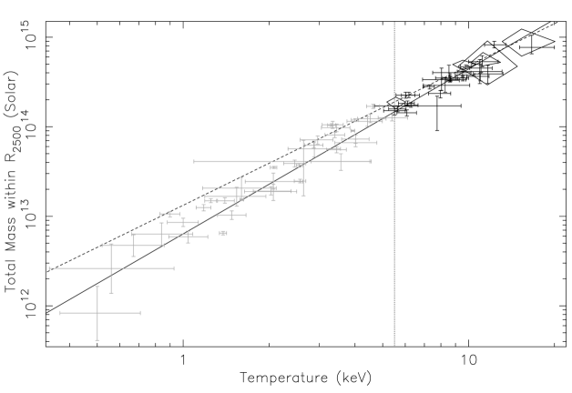
Figure 8: Total mass within $R_{\mathrm{2500}}$ as a function of emission-weighted temperature. The solid line is the best fitting power-law to the points above 5.5 keV (dotted vertical line), i.e. excluding the grey points. The diamonds are the data of Allen et al. (2001) and the dashed line is our best-fitting power-law to these data. See text for details.

7.3 The effects of non-isothermality

To investigate directly the effects of neglecting spatial variations in gas temperature, we have generated an additional set of isothermal models for our sample, i.e. with $\alpha=0$, for a linear $T(r)$, or $\gamma=1$, for a polytropic IGM. We have used the values of $\overline{T}$ already determined for the six different methods described above – with associated errors – to define the constant value. These isothermal models have then been subjected to an identical analysis to the original set, in order to provide a fair comparison of results.

Figure 9: Total mass as a function of emission-weighted temperature, evaluated within 0.3$R_{\mathrm{200}}$, for an isothermal IGM (method A^′). The solid line represents the best-fitting power law. See lower half of Table 2 for further details.

Fig. 9 shows the  relation for the isothermal sample derived using temperatures from method A (referred to as A^′). It can be seen that the convex shape evident in panel A of Fig. 7 is largely absent, and that a tighter relation about the best-fitting line is observed. The parameters of this power law fit are given in the lower half of Table 2, together with equivalent data for the other five isothermal  samples. Within 0.3$R_{\mathrm{200}}$ the logarithmic slope increases marginally for the isothermal models, but within the errors, for each of the three methods of measuring $\overline{T}$. However, for the two emission-weighted methods, the normalization increases by $\sim$15 per cent, although it is unchanged for the mass-weighted $\overline{T}$. Similar behaviour is observed for the  data evaluated within $R_{\mathrm{200}}$: the logarithmic slope is slightly steepened for the isothermal case, and the normalization is increased – for the emission-weighted methods – by $\sim$30 per cent. However, the mass-weighted normalization decreases by 15 per cent, compared to the non-isothermal models.

It is clear from this that the assumption of isothermality leads to an overestimate of the total mass within $R_{\mathrm{200}}$, when an emission-weighted method is used to calculate $\overline{T}$. A similar conclusion was reached by Horner et al. (1999), for a sample of 12 clusters, who found that isothermality overestimated the mass by a factor of 1.7 – a result confirmed by Neumann & Arnaud (1999). The latter authors found that the cumulative mass within a given radius for an isothermal cluster is significantly steeper than that of a cluster with a polytropic index of 1.25 (a value typical of the systems in our sample – see Table LABEL:tab:sample), with the intersection of the two occurring at $\sim$0.35$R_{\mathrm{200}}$. Consequently, the isothermal assumption over-predicts the mass for 96 per cent of the cluster volume.

Neglecting temperature gradients in the IGM appears to have little or no effect on the logarithmic slope of the  relation and, once again, the observed slopes are in good agreement between the three different methods of calculating $\overline{T}$. This is in contrast to the prediction of Horner et al. (1999), who suggested that the assumption of isothermality leads to a steepening in the  slope, which would otherwise be self-similar (i.e. 3/2). However, they base this conclusion on an analysis of a small sample (12 systems), with data drawn from a number of different sources in the literature. We also find that the rms scatter about the best fit  relations is significantly reduced in our isothermal models, and fully consistent with that expected from the statistical errors. We conclude that a power law seems to provide a good description of the  relation for an isothermal IGM.

Figure 10: Upper panel: Gas fraction within $R_{\mathrm{200}}$ as a function of emission-weighted temperature (within $R_{\mathrm{200}}$ – method ‘D’). Lower panel: Gas fraction within $R_{\mathrm{200}}$ for an isothermal IGM. The dotted lines show the unweighted mean of the whole sample.

The overestimation of the total mass for the isothermal case leads to a corresponding underestimation in the total gas fraction within $R_{\mathrm{200}}$, shown in Fig. 10. The unweighted mean gas fraction for the whole sample is $(0.110\pm 0.01)h_{\mathrm{70}}^{-\frac{3}{2}}$, as compared to $(0.134\pm 0.01)h_{\mathrm{70}}^{-\frac{3}{2}}$ for the non-isothermal case. It can also be seen that the scatter about the mean is lower for the isothermal case, although the apparent drop at $\sim$1 keV, seen in Fig. 10, is still noticeable. The most obvious outlier on this graph is the galaxy NGC 1553 (the left-most point). For this system, the isothermal model results in a significantly lower $f_{\mathrm{gas}}$, which greatly increases its distance from the sample mean.

7.4 Virial radius

The precise location of the outer boundary of a virialized halo is difficult to quantify and is very rarely directly observable. The virial radius is dependent on the mean density of the Universe when the halo was formed, as well as the adopted cosmology (Lacey & Cole, 1993). Clearly it is important to be able to define this quantity reliably, since we assume that self-similar haloes will have identical properties when scaled by $R_{\mathrm{v}}$. The radius enclosing a mean overdensity of 200 ($R_{\mathrm{200}}$) is proportional to $R_{\mathrm{v}}$ in any given cosmology – and lies within $R_{\mathrm{v}}$ for all reasonable cosmologies (Bryan & Norman, 1998) – and scales in a identical way (Navarro et al., 1995). However, previous studies have not always been able to determine $R_{\mathrm{200}}$, and so have relied on other means to estimate this quantity. A tight relationship between $T_{\mathrm{ew}}$ and $R_{\mathrm{v}}$ (and hence $R_{\mathrm{200}}$) is expected, as both these quantities reflect the depth of the gravitational potential well in a virialized halo; self-similarity predicts that $R_{\mathrm{v}}\ \propto\sqrt{T_{\mathrm{ew}}}$ (c.f. the size-temperature relation, Mohr & Evrard 1997). This proportionality has been confirmed in ensembles of simulated clusters, which provide a value for the normalization in the relation. One such example is the work of Navarro et al. (1995), who deduce that

$$R_{\mathrm{200}}=0.813\left(\frac{T}{\rm{keV}}\right)^{\frac{1}{2}}(1+z)^{-\frac{3}{2}}h_{\mathrm{70}}^{-1}\mbox{~{}Mpc}.$$ (9)

However, their simulations only included adiabatic compression and shock heating, and did not allow for the effects of energy injection.

The correspondence between our values of $R_{\mathrm{200}}$ as determined from the overdensity profile (listed in Table LABEL:tab:sample) and those calculated with equation 9 is shown in Fig. 11. It can be seen that there is significant deviation from the locus of equality between these quantities, marked by the solid line. The largest discrepancy is observed in the smallest haloes, indicating that the NFW equation significantly over-predicts $R_{\mathrm{200}}$ in these systems (the effect of extrapolation bias is addressed in section 7.5). This is to be expected, given that $T_{\mathrm{ew}}$ for these objects is most likely to be susceptible to bias from non-gravitational heating. To explore the reasons for the disagreement between the two methods for calculating $R_{\mathrm{200}}$, we have examined the role of temperature gradients as the source of the scatter, given their importance in calculating the gravitating mass (see equation 4). We have defined a simple, quantitative measure of the departure from isothermality, which, as has already been seen, can exert a significant influence on scaling properties (section 7.3). We use the ratio $T(0)/T(0.3R_{\mathrm{200}})$, as this is very sensitive to the presence of a temperature gradient, and the two distances involved bracket the region of interest used to calculate $T_{\mathrm{ew}}$.

Figure 11: Predicted $R_{\mathrm{200}}$ from the NFW formula (equation 9) plotted against measured $R_{\mathrm{200}}$. The solid line indicates the line of equality.

Figure 12: The ratio between measured $R_{\mathrm{200}}$ and $R_{\mathrm{200}}$ from the NFW formula, as a function of the ratio between $T(r)$ at $R=0$ and $R=0.3R_{\mathrm{200}}$. Error bars have been omitted for clarity. The lines of equality on both axes are marked; the solid line represents the locus of isothermality.

The relationship between this quantity and the ratio of the measured $R_{\mathrm{200}}$ divided by the NFW predicted value, is shown in Fig. 12. There is clearly a strong anti-correlation between these quantities, significant at the $6.9\sigma$ level. Even with the two most extreme points removed (the left and right-most points on the graph), the significance of the relation drops only slightly, to $6.4\sigma$. It can be seen that the most isothermal systems (clustered around the solid vertical line) scatter around the line of equality between the two measurements of $R_{\mathrm{200}}$. This demonstrates that the NFW formula is valid only for nearly isothermal haloes, and that it otherwise over-predicts $R_{\mathrm{200}}$ for the most common case of a radially decreasing temperature profile.

7.5 Extrapolation bias

Our analysis relies on the validity of extrapolating analytical profiles fitted to an inner region of the data, in order to compensate for the emission which is undetected. However, since the extrapolation is, in general, greater for smaller systems, there is a potential for introducing a systematic bias in our fitting. This is particularly true of the slope of the gas density profile, which is best constrained by the emission from outer regions of the X-ray halo, and which has been found to vary significantly with temperature (see section 7.1). The work of Vikhlinin et al. (1999) has shown that there is evidence of a slight steepening of the gas density logarithmic slope with radius. Such behaviour would naturally lead to lower values of $\beta$ being inferred for cooler systems, since their smaller haloes would be detectable to a smaller fraction of $R_{\mathrm{v}}$, compared to those of more massive clusters. This effect could therefore explain part of the observed correlation between $\beta$ and $T_{\mathrm{ew}}$. To explore the effects of extrapolation on our data, we have performed a series of fits to the surface brightness profiles of two clusters (Abell 1795 & Abell 2029), investigating the role of the outer radius of the fitted data in constraining the fit parameters.

These clusters were selected as they are rich systems (and hence relatively unaffected by energy injection), with high quality data ($\sim$100,000 and 30,000 counts, respectively), that cover a fairly large angular extent. This allows us to trace the emission to a large fraction of $R_{\mathrm{v}}$ and means we can analyse a spatial subset of the data, without approaching the resolution limits of the instrument. In addition, we have chosen systems which have cooling flow emission confined to as small a region as possible, compared to the gas halo core size, so as to minimize the bias this contamination can have on our results.

Since we are aiming in this section only to explore the behaviour of the gas density logarithmic slope as a function of radius, we have adopted a different approach to that described in section 3.5. Rather than applying a full deprojection analysis to the data, we have fitted 1-dimensional, azimuthally-averaged, surface brightness profiles for each cluster. This method permits a much more direct investigation of the gas density index in the outer regions of the halo and allows us use a quantitative measure of goodness-of-fit, based on the $\chi^{2}$ criterion.

We obtained azimuthally-averaged surface brightness profiles for both clusters, from ROSAT PSPC data, in the following way. An image of the cluster was extracted in the 0.2–2.4 keV band, and point sources above 4.5$\sigma$ significance were masked out. Using the master veto rate, the contribution to the background from particles was subtracted, and the image was then ‘flattened’ by dividing by the corresponding exposure map, to correct for the effects of vignetting. An estimate of the astrophysical background was obtained, based on an annulus extracted from beyond the cluster emission, with the PSPC support spokes removed. Point sources were also masked out from the annulus, and the remaining counts were extrapolated across the field and subtracted from the source image. Finally, a radial profile was extracted – centred on the peak in the X-ray emission – in a series of fixed-width annuli, with a minimum of 50 counts per bin (see Fig. 13).

A King profile function (equation 6) was fitted to the data, using the qdp package (Tennant, 1999), and all three parameters were left free to vary. A small central region of the data was excised, to prevent emission from the cooling flow biasing the results. The fitting was repeated for a subset of the data, excluding emission beyond a fixed radius, $R_{\mathrm{outer}}$, so as to investigate any systematic variation in $\beta$ with radius. The results of these fits are summarised in table 3, and the best-fitting model to the whole image is shown, together with the data points, in Fig. 13.

It can be seen from Table 3 that there is only marginal evidence for a systematic trend in $\beta$ with radius for A2029, with a large overlap between the confidence regions. However, A1795 seems to show a significantly lower $\beta$ (0.70) for the innermost 9′, as compared to the profile fitted out to 17′. An explanation of this apparent flattening can be found in the core radius, which is significantly smaller – 2.2′, as compared to 3.7′ for the whole profile. This behaviour is an artefact of the excised central cooling region, which is comparable in size to the gas core in the IGM. Consequently, $r_{\mathrm{c}}$ is biased when a large part of the outer profile is excluded from the fit – and this propagates through to the best-fitting $\beta$ value. This is confirmed by the bottom row in Table 3, which lists the results of re-fitting the innermost 9′ with $r_{\mathrm{c}}$ frozen at the best-fitting value from the full, 17′ profile: the corresponding $\beta$ (0.83) is, in fact, identical to the slope for the whole profile. This problem is particularly pronounced for A1795 due to its fairly large cooling flow: the excised central region amounts to $\sim$15 per cent of $R_{\mathrm{200}}$. The radius of the cooling flow in A2029 is only about 10 per cent of $R_{\mathrm{200}}$, a value which is more typical of groups, and hence the potential for bias in $r_{\mathrm{c}}$ is minimal.

Lewis et al. (2000) find a similar tendency for $r_{\mathrm{c}}$ and $\beta$ to decrease, when fitting truncated radial profiles of simulated clusters. Similarly, their analysis excludes a central portion of the data, corresponding to emission from either the central cluster galaxy or a cooling flow. They also claim to find a steepening in the logarithmic slope of the gas density with radius in the outer regions, as reported by Vikhlinin et al. (1999); however, this discrepancy is only evident in the vicinity of the virial radius – a region rarely probed by observations of even the hottest clusters. In any case, it is clear that, even if such a steepening is a significant effect, it is not able to introduce large systematic relative biases between groups and clusters in our analysis.

Cluster name	Temperature	$R_{\mathrm{outer}}$	$R_{\mathrm{outer}}$/$R_{\mathrm{200}}$	Normalization	$\beta$	$r_{\mathrm{c}}$	red. $\chi^{2}$/dof
	(keV)	(arcmin)		(ct s-1/degree2)		(arcmin)
A2029	9.80	18	0.68	$294^{+9}_{-33}$	$0.73^{+0.02}_{-0.01}$	$2.51^{+0.20}_{-0.20}$	1.25/23
		12	0.45	$356^{+74}_{-53}$	$0.70^{+0.02}_{-0.02}$	$2.17^{+0.24}_{-0.24}$	1.35/13
		9	0.34	$399^{+130}_{-77}$	$0.68^{+0.03}_{-0.03}$	$1.99^{+0.31}_{-0.32}$	1.72/8
A1795	8.54	17	0.60	$173^{+21}_{-17}$	$0.83^{+0.02}_{-0.02}$	$3.72^{+0.25}_{-0.24}$	1.04/50
		12	0.42	$209^{+41}_{-30}$	$0.79^{+0.03}_{-0.03}$	$3.26^{+0.33}_{-0.33}$	1.18/30
$\dagger$		9	0.32	$401^{+364}_{-130}$	$0.70^{+0.04}_{-0.03}$	$2.18^{+0.53}_{-0.59}$	1.09/18
$r_{\mathrm{c}}$ fixed⋆		9	0.32	$169^{+5}_{-5}$	$0.83^{+0.01}_{-0.01}$	$3.72$	1.49/19

Table 3: Summary of results for the 1-dimensional surface brightness fitting within different radii. Errors are 1$\sigma$. A central region of the data was excluded to avoid contamination of by cooling flow emission; the radii of exclusion were 2.7′ & 4′ for A2029 & A1795, respectively. $\dagger$This fit was noticeably biased by the excised central region of the data and was repeated: ^⋆ indicates that the core radius was frozen at its previously-determined best-fit value to the whole profile (see text for details).

Figure 13: Azimuthally averaged surface brightness profiles for A1795 (left panel) and A2029 (right panel). The solid line indicates the best-fitting model (see text for details).

8 Discussion

It is clear from the scaling properties we have examined, that virialized systems do not exhibit self-similar behaviour. The $\beta-T$ relation and the gas fraction data reveal a flattening of the gas density profiles, which is most obvious in the group regime. These observations are consistent with energy injection into the IGM by non-gravitational means. However, three questions remain unanswered. Firstly, what caused this heating; secondly, when did it take place and, thirdly, is self-similarity broken only below a certain critical temperature, or does the transition occur gradually?

There are three main candidates for the origin of the self-similarity breaking. Both galaxy winds (e.g. Lloyd-Davies et al., 2000) and AGN heating (e.g. Wu et al., 2000) are able to inject energy at roughly the levels required to raise the entropy of gas in the central regions of the IGM. However, the role of gas cooling in imposing an entropy floor (e.g. Muanwong et al., 2001) could also be significant. Although our results in this paper provide no means of discriminating between the first two options, our data do allow us to address the viability of cooling. The cooling hypothesis is offered some support by our gas fraction results: the variation in $f_{\mathrm{gas}}$ with $T_{\mathrm{ew}}$ shown in figures 5 & 6, is consistent with the loss of gas required in the cool systems if cooling is to have a significant effect. On the other hand, there is no evidence that groups have an excessive total $L_{\mathrm{B}}$ compared to clusters, which would be expected if the cooling gas ultimately formed stars (Helsdon & Ponman, 2002). This may indicate that the $f_{\mathrm{gas}}$ trend is due to gas being displaced to larger radius by the effects of energy injection, as demonstrated by the simulations of Metzler & Evrard (1997), for example.

However, it should be noted that simulations which model the effects of cluster mergers can generate a similarly extended gas distribution, without energy injection from non-gravitational processes (Navarro & White, 1993; Pearce et al., 1994). Similarly, while the large intrinsic scatter in the $\beta-T$ relation may reflect a difference in the level of energy injection between haloes, it can also be attributed to the effects of hierarchical assembly: Cavaliere et al. (1999) predict a $\beta-T$ relation with a 2$\sigma$ scatter envelope, resulting from merging histories, which is in qualitative agreement with the data in Fig. 3.

The second question raises two possibilities; either the heating took place prior to halo collapse (so called ‘external’ or ‘pre-’heating), or most energy injection occurred after virialization (internal heating). Although a rather simplistic distinction, these two scenarios will manifest themselves in different ways on cluster properties, given the effect of injecting energy into a medium in which a significant density gradient has already been established. For example, preheating will tend to weaken the shock boundary and move it outwards as compared to internal heating (Tozzi et al., 2000). Since this boundary marks the point where the gas fraction fades into the universal value, this amounts to an observable signature. The evidence from $f_{\mathrm{gas}}$ is tentative, given the extrapolation uncertainties, but there is indication of a systematic variation in the total gas fraction within $R_{\mathrm{200}}$ with $T_{\mathrm{ew}}$. Observations of the X-ray background suggest that the heating phase took place over a time-scale of $\sim$10⁷ yr (Pen, 1999), although the epoch of energy injection is not constrained. Conversely, observations of the entropy floor (Ponman et al., 1999; Lloyd-Davies et al., 2000) place a strict upper limit on $z_{\mathrm{preh}}$, the redshift at which the preheating epoch could have taken place, of $z_{\mathrm{preh}}\la 10$.

The question of on what mass scale the effects of self-similarity breaking occur is more readily answered with our large sample. Whereas previous work has pointed to a sharp transition between groups and clusters, our results do not offer much support for this hypothesis. The analytical approach of Dos Santos & Doré (2002) shows that the two mass regimes can be unified with a simple model that incorporates energy injection from non-gravitational processes. Their predicted scaling relations show a gradual steeping of  and $L-T_{\mathrm{X}}$, with decreasing temperature, and indicate that accretion shocks cannot be completely suppressed in groups. Our measured  data offer some support for a convex relation, as opposed to a broken power law, but the scatter is rather large. Whilst higher quality data from XMM-Newton and Chandra will doubtless shed some light on this issue, the greatest uncertainty lies in the systematic bias associated with extrapolation to $R_{\mathrm{200}}$: it is necessary to trace the X-ray haloes of nearby groups out to $R_{\mathrm{v}}$ in order to resolve the issue satisfactorily, and this calls for observations with a wider field-of-view.

8.1 Galaxies vs. groups

In a CDM Universe, the formation of structure proceeds in a bottom-up fashion, with the smallest haloes virializing initially and subsequent merging activity leading to the hierarchical assembly of progressively larger haloes (e.g. Blumenthal et al., 1984). Consequently, the smallest objects tend to be older, having collapsed at an earlier epoch. This then leads to differences in the scaling properties, as a result of the higher density of the Universe at that time (e.g. the  relation normalization). However, in the context of a preheating prescription, invoked to explain the breaking of self-similarity in galaxy groups, the timing of this early formation epoch is critical; it is possible that these objects virialized prior to the preheating phase. This would give rise to behaviour more consistent with massive clusters of galaxies, which are sufficiently large as to be insensitive to the effects of energy injection. One possible candidate for the origin of this preheating is population III stars, whose formation precedes even that of galaxies, which may also have contributed to the enrichment of the IGM (e.g. Loewenstein, 2001).

As has already been seen, the properties of the galaxy-sized haloes in this sample appear to differ from those of groups of a similar temperature. Specifically, the gas density index ($\beta$) is rather steeper than expected from a simple extrapolation of the $\beta-T$ relation for the whole sample. In addition, the S0 galaxy NGC 1553 lies noticeably below the  relation. This can be understood in terms of a large discrepancy between its redshift of formation and observation: there is a bias towards observing nearby objects of small mass, but these are likely to have formed earliest of all sized haloes. For a given halo mass, the virial temperature is proportional to $(1+z_{\mathrm{f}})$ and so, for NGC 1553, a value of $z_{\mathrm{f}}\sim 3$–4 would increase $T_{\mathrm{ew}}$, and push it to the right of the  relation, as observed. Alternatively, the discrepancy can be attributed to the effects of non-gravitational heating on $T_{\mathrm{ew}}$ caused, for example, by outflows from within the galaxy itself: a value of $T_{\mathrm{ew}}\simeq 0.3\mbox{~{}keV}$ (compared to the actual value of 0.5 keV) would bring the point back on the best-fitting  relation for the whole sample. This explanation is further supported by its $L_{\mathrm{X}}$/$L_{\mathrm{B}}$, which is low enough for the stellar population in the galaxy to have significantly influenced its X-ray halo (e.g. Pellegrini & Ciotti, 1998).

In fact, the behaviour of NGC 1553 is sufficiently unusual that it points to an alternative formation mechanism to that which is usually invoked for hot gas in groups and clusters. For example, the halo could have been built from supernova-driven winds, originating in its own stellar population (e.g. Ciotti et al., 1991), rather than from primordial material . This explanation is supported by its $L_{\mathrm{X}}$/$L_{\mathrm{B}}$, and may explain the anomalously steep $\beta$ index, which would otherwise be flattened by the effects of energy injection prior to collapse.

In contrast, the position of the elliptical galaxy NGC 6482 on the  relation is fully consistent with the best fit line to the whole sample. This is not surprising, as it is likely that this object is a fossil group and hence will exhibit group-type behaviour. What is certain is that this must be a very old system, given the long time-scale for orbital decay and merging of the galaxy members. Although not as discrepant as NGC 1553, NGC 6482 shows some suggestion that its $\beta$ index may be high for its temperature. This could indicate that it formed sufficiently early to have been relatively unaffected by a phase of energy injection, that would have occurred prior to the formation of most larger objects. There is no doubt that its halo must be predominantly primordial – its $L_{\mathrm{X}}$/$L_{\mathrm{B}}$ is sufficiently high that the influence of its stellar population is negligible, in terms of contributing to the total gas mass.

Given an early formation epoch, consistent with hierarchical formation, coupled with a correspondingly larger mean density, it is particularly important to consider the cooling time of the X-ray gas. At a radius of 0.1$R_{\mathrm{200}}$, NGC 1553 has a gas cooling time ($t_{\mathrm{cool}}$) of $\sim$6 Gyr and NGC 6482 has $t_{\mathrm{cool}}\simeq 3$ Gyr. For comparison, the cooling times of the next two coolest systems in our sample – HCG 68 and NGC 1395 – are 18 Gyr and $\sim$25 Gyr, respectively. In the case of NGC 1553, this implies that some form of heating mechanism must have prevented significant gas cooling, if its halo was formed before $z=1$ (corresponding to a light travel time of roughly 6 Gyr). This is also supported by the fact that there appears to be no evidence of strong cooling in the core, where the density is even higher. Energy injection from galaxy winds could provide the heating mechanism necessary to explain this result, as suggested above. For NGC 6482, some mechanism is also needed to prevent catastrophic gas cooling, which is not observed even in the core, given that this fossil group must be a very old system. Once again, its high $L_{\mathrm{X}}$/$L_{\mathrm{B}}$ rules out a significant heating contribution from supernova-driven winds. However, there is some evidence of an AGN component in this galaxy (Goudfrooij et al., 1994), which may provide a suitable reheating mechanism to prevent the establishment of a cooling flow.

9 Conclusions

We have studied the scaling properties of the X-ray emitting gas and gravitating mass of a large sample of clusters, groups and galaxy-size haloes. The 3-dimensional variations in gas density and temperature – corrected for contamination from cooling flows – are parametrized analytically, allowing us determine all derived quantities in a self-consistent manner. We have derived virial radii and emission-weighted temperatures from these models and are able to extrapolate the properties of the data to measure them at fixed fractions of $R_{\mathrm{v}}$. We have also analysed an identical set of isothermal models, to investigate the effects of neglecting spatial variations in the temperature of the IGM. We summarise our main findings below.

1. Beta varies strongly with temperature, although there is evidence that galaxy-sized haloes do not follow this trend. We find a best fit power law relation of the form $\beta=(0.44\pm 0.06)T^{0.20\pm 0.03}$.

2. There is a $6\sigma$ correlation between $f_{\mathrm{gas}}$ within 0.3$R_{\mathrm{200}}$ and temperature, consistent with the variation in $\beta$. This trend is weakened only slightly (to $5.4\sigma$) by extrapolating the gas fraction to $R_{\mathrm{200}}$ although, above 4 keV, the significance of this correlation drops to 3.2$\sigma$. The mean $f_{\mathrm{gas}}$ within $R_{\mathrm{200}}$ for the systems hotter than 4 keV is $(0.163\pm 0.01)h_{\mathrm{70}}^{-\frac{3}{2}}$, compared to $(0.134\pm 0.01)h_{\mathrm{70}}^{-\frac{3}{2}}$ for the whole sample. Under the assumption of isothermality, the scatter between $f_{\mathrm{gas}}$ at $R_{\mathrm{200}}$ and $T_{\mathrm{ew}}$ is reduced, as is the normalization, giving a mean for the whole sample of $(0.110\pm 0.01)h_{\mathrm{70}}^{-\frac{3}{2}}$.

3. Observations of the variation in gas fraction as a function of radius in our sample reveal a systematic trend in gas fraction with temperature in all but the central regions (≲0.3$R_{\mathrm{200}}$). This is consistent with the observed trend in $f_{\mathrm{gas}}$ with $T_{\mathrm{ew}}$.

4. In our study of the  relation, we employ two additional methods of calculating the average system temperature, one of which excludes the central region, another weighting the temperature with gas density rather than emissivity. We apply our three different methods within both 0.3$R_{\mathrm{200}}$ and $R_{\mathrm{200}}$, for both mass and $\overline{T}$, to give a total of six  relations. We find that the logarithmic slope of the relation is steeper within 0.3$R_{\mathrm{200}}$ but that, even within $R_{\mathrm{200}}$, it is inconsistent with self-similarity. There is close agreement between the measured slopes found for each of the three different prescriptions for $\overline{T}$. For the emission-weighted $\overline{T}$, within $R_{\mathrm{200}}$, we find $M=2.34\times 10^{13}\times T^{(1.84\pm 0.06)}$ $M_{\mathrm{\odot}}$. We find that the effect of assuming isothermality on the slope is negligible, but the normalization increases by 15 and 30 per cent for 0.3$R_{\mathrm{200}}$ and $R_{\mathrm{200}}$, respectively (c.f. Neumann & Arnaud, 1999; Horner et al., 1999), indicating that the total gravitating mass is significantly overestimated in our data when temperature gradients are neglected. In addition, the scatter in the relation is reduced (and fully consistent with the parameter errors) compared to the non-isothermal case. The corresponding best fit relation is given by $M=3.02\times 10^{13}\times T^{(1.89\pm 0.04)}$ $M_{\mathrm{\odot}}$.

5. The relation between $R_{\mathrm{200}}$ and $T_{\mathrm{ew}}$, as deduced from simulated clusters (Navarro et al., 1995) deviates systematically from the measured values of $R_{\mathrm{200}}$, as inferred from the overdensity profile. We find a strong negative correlation between the ratio of the NFW predicted $R_{\mathrm{200}}$ to our measured values and a quantitative measure of non-isothermality ($T(0)/T(0.3R_{\mathrm{200}})$). We show that only in the absence of a temperature gradient do the methods agree.

6. We address the issue of systematic bias associated with the extrapolation of the X-ray data to $R_{\mathrm{200}}$, by fitting azimuthally averaged surface brightness profiles for two clusters, within different outer radii. We find no evidence for a significant variation in $\beta$ with cluster radius and conclude that the flatter gas density profiles of cooler systems cannot be attributed to the generally smaller angular range over which data are available for these objects.

7. We find that the two galaxies in the sample display unusual properties. We have selected these objects on the basis of a lack of associated group or cluster halo emission, which can contaminate the galaxy halo flux. The S0 galaxy, NGC 1553 has a steep $\beta$ index and falls to the right of the main  relation, indicative of an early formation epoch ($z_{\mathrm{f}}\sim$ 3–4) – which causes haloes of a given mass to be hotter than those collapsing at later times. It is also possible that $T_{\mathrm{ew}}$ for this galaxy may have been artificially raised, probably by supernova-driven outflows from its stellar population. The elliptical galaxy NGC 6482 also shows a rather steep gas density profile, but otherwise exhibits group-like behaviour, consistent with a classification as a ‘fossil’ group.

References

- Allen et al. (2001) Allen S. W., Schmidt R. W., Fabian A. C., 2001, MNRAS, 328, L37
- Arnaud & Evrard (1999) Arnaud M., Evrard A. E., 1999, MNRAS, 305, 631
- Arnaud et al. (2001) Arnaud M., Neumann D. M., Aghanim N., Gastaud R., Majerowicz S., Hughes J. P., 2001, A&A, 365, L80
- Bevington (1969) Bevington P. R., 1969, Data reduction and error analysis for the physical sciences. New York: McGraw-Hill, 1969
- Blanton et al. (2001) Blanton E. L., Sarazin C. L., Irwin J. A., 2001, ApJ, 552, 106
- Blumenthal et al. (1984) Blumenthal G. R., Faber S. M., Primack J. R., Rees M. J., 1984, Nature, 311, 517
- Boggs et al. (1989) Boggs P. T., Byrd R. H., Donaldson J. R., Schnabel R. B., 1989, ACM Trans. Math. Software, 15(4), 348
- Boggs et al. (1992) Boggs P. T., Byrd R. H., Rogers J. E., Schnabel R. B., 1992, User’s Reference Guide for odrpack Version 2.01
- Böhringer et al. (2002) Böhringer H., Matsushita K., Churazov E., Ikebe Y., Chen Y., 2002, A&A, 382, 804
- Bryan & Norman (1998) Bryan G. L., Norman M. L., 1998, ApJ, 495, 80
- Cash (1979) Cash W., 1979, ApJ, 228, 939
- Cavaliere & Fusco-Fermiano (1976) Cavaliere A., Fusco-Fermiano R., 1976, A&A, 49, 137
- Cavaliere et al. (1999) Cavaliere A., Menci N., Tozzi P., 1999, MNRAS, 308, 599
- Ciotti et al. (1991) Ciotti L., Pellegrini S., Renzini A., D’Ercole A., 1991, ApJ, 376, 380
- David et al. (1995) David L. P., Jones C., Forman W., 1995, ApJ, 445, 578
- David et al. (2001) David L. P., Nulsen P. E. J., McNamara B. R., Forman W., Jones C., Ponman T., Robertson B., Wise M., 2001, ApJ, 557, 546
- De Grandi & Molendi (2002) De Grandi S., Molendi S., 2002, ApJ, 567, 163
- Dos Santos & Doré (2002) Dos Santos S., Doré O., 2002, A&A, 383, 450
- Ebeling et al. (1998) Ebeling H., Edge A. C., Böringer H., Allen S. W., Crawford C. S., Fabian A. C., Voges W., Huchra J. P., 1998, MNRAS, 301, 881
- Ebeling et al. (1996) Ebeling H., Voges W., Böhringer H., Edge A. C., Huchra J. P., Briel U. G., 1996, MNRAS, 281, 799
- Edge & Stewart (1991) Edge A. C., Stewart G. C., 1991, MNRAS, 252, 414
- Evrard et al. (1996) Evrard A. E., Metzler C. A., Navarro J. F., 1996, ApJ, 469, 494
- Eyles et al. (1991) Eyles C. J., Watt M. P., Bertram D., Church M. J., Ponman T. J., Skinner G. K., Willmore A. P., 1991, ApJ, 376, 23
- Fabian (1994) Fabian A. C., 1994, ARA&A, 32, 277
- Fabricant et al. (1984) Fabricant D., Rybicki G., Gorenstein P., 1984, ApJ, 286, 186
- Fairley et al. (2000) Fairley B. W., Jones L. R., Scharf C., Ebeling H., Perlman E., Horner D., Wegner G., Malkan M., 2000, MNRAS, 315, 669
- Finoguenov et al. (2001) Finoguenov A., Arnaud M., David L. P., 2001, ApJ, 555, 191
- Finoguenov et al. (2000) Finoguenov A., David L. P., Ponman T. J., 2000, ApJ, 544, 188
- Finoguenov & Jones (2000) Finoguenov A., Jones C., 2000, ApJ, 539, 603
- Finoguenov & Ponman (1999) Finoguenov A., Ponman T. J., 1999, MNRAS, 305, 325
- Finoguenov et al. (2001) Finoguenov A., Reiprich T. H., Böhringer H., 2001, A&A, 368, 749
- Goffe et al. (1994) Goffe W. L., Ferrier G. D., Rogers J., 1994, J. Econometrics, 60, 65
- Goudfrooij et al. (1994) Goudfrooij P., Hansen L., Jorgensen H. E., Norgaard-Nielsen H. U., 1994, A&AS, 105, 341
- Helsdon & Ponman (2000) Helsdon S. F., Ponman T. J., 2000, MNRAS, 315, 356
- Helsdon & Ponman (2002) Helsdon S. F., Ponman T. J., 2002, MNRAS, accepted (astro-ph/0212046)
- Helsdon et al. (2001) Helsdon S. F., Ponman T. J., O’Sullivan E., Forbes D. A., 2001, MNRAS, 325, 693
- Hobbs & Willmore (1997) Hobbs I. S., Willmore A. P., 1997, MNRAS, 289, 685
- Horner et al. (1999) Horner D. J., Mushotzky R. F., Scharf C. A., 1999, ApJ, 520, 78
- Irwin & Bregman (2000) Irwin J. A., Bregman J. N., 2000, ApJ, 538, 543
- James (1998) James F., 1998, CERN Program Library Long Writeup D506
- Johnstone et al. (2002) Johnstone R. M., Allen S. W., Fabian A. C., Sanders J. S., 2002, MNRAS, 336, 299
- Jones & Forman (1984) Jones C., Forman W., 1984, ApJ, 276, 38
- Jones & Forman (1999) Jones C., Forman W., 1999, ApJ, 511, 65
- Jones et al. (2000) Jones L. R., Ponman T. J., Forbes D. A., 2000, MNRAS, 312, 139
- Kim et al. (1992) Kim D.-W., Fabbiano G., Trinchieri G., 1992, ApJ, 393, 134
- Knight & Ponman (1997) Knight P. A., Ponman T. J., 1997, MNRAS, 289, 955
- Lacey & Cole (1993) Lacey C., Cole S., 1993, MNRAS, 262, 627
- Lewis et al. (2000) Lewis G. F., Babul A., Katz N., Quinn T., Hernquist L., Weinberg D. H., 2000, ApJ, 536, 623
- Lloyd-Davies et al. (2000) Lloyd-Davies E. J., Ponman T. J., Canon D. B., 2000, MNRAS, 315, 689
- Loewenstein (2001) Loewenstein M., 2001, ApJ, 557, 573
- McNamara et al. (2000) McNamara B. R., Wise M., Nulsen P. E. J., David L. P., Sarazin C. L., Bautz M., Markevitch M., Vikhlinin A., Forman W. R., Jones C., Harris D. E., 2000, ApJ, 534, L135
- Markevitch (1996) Markevitch M., 1996, ApJ, 465, L1
- Markevitch (1998) Markevitch M., 1998, ApJ, 504, 27
- Markevitch et al. (1998) Markevitch M., Forman W. R., Sarazin C. L., Vikhlinin A., 1998, ApJ, 503, 77
- Markevitch & Vikhlinin (1997) Markevitch M., Vikhlinin A., 1997, ApJ, 474, 84
- Markevitch & Vikhlinin (2001) Markevitch M., Vikhlinin A., 2001, ApJ, 563, 95
- Markevitch et al. (1999) Markevitch M., Vikhlinin A., Forman W. R., Sarazin C. L., 1999, ApJ, 527, 545
- Metzler & Evrard (1997) Metzler C. A., Evrard A. E., 1997, preprint, (astro-ph/9710324)
- Mewe et al. (1986) Mewe R., Lemen J. R., van den Oord G. H. J., 1986, A&A, 65, 511
- Mohr & Evrard (1997) Mohr J. J., Evrard A. E., 1997, ApJ, 491, 38
- Mohr et al. (1999) Mohr J. J., Mathieson B., Evrard A. E., 1999, ApJ, 517, 627
- Muanwong et al. (2001) Muanwong O., Thomas P. A., Kay S. T., Pearce F. R., Couchman H. M. P., 2001, ApJ, 552, L27
- Mulchaey & Zabludoff (1998) Mulchaey J. S., Zabludoff A. I., 1998, ApJ, 496, 73
- Mulchaey & Zabludoff (1999) Mulchaey J. S., Zabludoff A. I., 1999, ApJ, 514, 133
- Navarro et al. (1995) Navarro J. F., Frenk C. S., White S. D. M., 1995, MNRAS, 275, 720
- Navarro et al. (1997) Navarro J. F., Frenk C. S., White S. D. M., 1997, ApJ, 490, 493
- Navarro & White (1993) Navarro J. F., White S. D. M., 1993, MNRAS, 265, 271
- Neumann & Arnaud (1999) Neumann D. M., Arnaud M., 1999, A&A, 348, 711
- Nevalainen et al. (2001) Nevalainen J., Kaastra J., Parmar A. N., Markevitch M., Oosterbroek T., Colafrancesco S., Mazzotta P., 2001, A&A, 369, 459
- Nevalainen et al. (2000) Nevalainen J., Markevitch M., Forman W., 2000, ApJ, 532, 694
- Pearce et al. (1994) Pearce F. R., Thomas P. A., Couchman H. M. P., 1994, MNRAS, 268, 953
- Pellegrini & Ciotti (1998) Pellegrini S., Ciotti L., 1998, A&A, 333, 433
- Pen (1999) Pen U., 1999, ApJ, 510, L1
- Peres et al. (1998) Peres C. B., Fabian A. C., Edge A. C., Allen S. W., Johnstone R. M., White D. A., 1998, MNRAS, 298, 416
- Ponman et al. (1994) Ponman T. J., Allan D. J., Jones L. R., Merrifield M., McHardy I. M., Lehto H. J., Luppino G. A., 1994, Nature, 369, 462
- Ponman et al. (1996) Ponman T. J., Bourner P. D. J., Ebeling H., Böhringer H., 1996, MNRAS, 283, 690
- Ponman et al. (1999) Ponman T. J., Cannon D. B., Navarro J. F., 1999, Nature, 397, 135
- Ritchie & Thomas (2002) Ritchie B. W., Thomas P. A., 2002, MNRAS, 329, 675
- Sarazin (1988) Sarazin C. L., 1988, X-ray emission from clusters of galaxies. Cambridge Astrophysics Series, Cambridge: Cambridge University Press, 1988
- Sato et al. (2000) Sato S., Akimoto F., Furuzawa A., Tawara Y., Watanabe M., Kumai Y., 2000, ApJ, 537, L73
- Stark et al. (1992) Stark A. A., Gammie C. F., Wilson R. W., Bally J., Linke R. A., Heiles C., Hurwitz M., 1992, ApJS, 79, 77
- Tamura et al. (2001) Tamura T., Bleeker J. A. M., Kaastra J. S., Ferrigno C., Molendi S., 2001, A&A, 379, 107
- Tennant (1999) Tennant A. F., 1999, The qdp/plt User’s Guide
- Tozzi et al. (2000) Tozzi P., Scharf C., Norman C., 2000, ApJ, 542, 106
- Vikhlinin et al. (1999) Vikhlinin A., Forman W., Jones C., 1999, ApJ, 525, 47
- Vikhlinin et al. (1999) Vikhlinin A., McNamara B. R., Hornstrup A., Quintana H., Forman W., Jones C., Way M., 1999, ApJ, 520, L1
- Voit & Bryan (2001) Voit G. M., Bryan G. L., 2001, Nature, 414, 425
- White (2000) White D. A., 2000, MNRAS, 312, 663
- White & Fabian (1995) White D. A., Fabian A. C., 1995, MNRAS, 273, 72
- Wu et al. (2000) Wu K. K. S., Fabian A. C., Nulsen P. E. J., 2000, MNRAS, 318, 889