Next-generation test of cosmic inflation

Abstract

The increasing precision of cosmological datasets is opening up new opportunities to test predictions from cosmic inflation. Here we study the impact of high precision constraints on the primordial power spectrum and show how a new generation of observations can provide impressive new tests of the slow-roll inflation paradigm, as well as produce significant discriminating power among different slow-roll models. In particular, we consider next-generation measurements of the Cosmic Microwave Background (CMB) temperature anisotropies and (especially) polarization, as well as new Lyman-$\alpha$ measurements that could become practical in the near future. We emphasize relationships between the slope of the power spectrum and its first derivative that are nearly universal among existing slow-roll inflationary models, and show how these relationships can be tested on several scales with new observations. Among other things, our results give additional motivation for an all-out effort to measure CMB polarization.

I Introduction

Over the last several years, extraordinary observational support has emerged for the idea that key features of our universe were formed by a period of cosmic inflation. During inflation, the universe enters a period of “superluminal expansion” which imprints certain features on the universe. The physical degree of freedom responsible for inflation, generically called the “inflaton”, has yet to find a comfortable home in fundamental theory, and there are many competing ideas for how fundamental aspects of inflation could play out. None the less, at the phenomenological level a standard picture of inflation has emerged.

From the observational point of view, the standard picture is defined by a set of observable characteristics that are the same across virtually all proposed models for the inflaton. The most well known predictions from the standard picture of inflation are that the universe has critical density (to within roughly one part in $10^{5}$), that the primordial perturbations are coherent, (leading, for example, to acoustic peaks in the microwave background power spectrum), and that the power spectrum of primordial perturbations is nearly scale invariant, with the tilt parameter $n_{s}$ constrained to be close to unity. A unique spectrum of coherent gravitational waves is also predicted, which could eventually come within range of direct gravitational wave detectors, and which could also be observed indirectly via signals in the microwave background polarization.

But inflation makes many more predictions than these. Specifically, a given model for the inflaton will predict a detailed shape for the primordial power spectrum that goes way beyond what can be described simply by a single tilt parameter. The detailed shape of the power spectrum is a reflection of the particular evolution of the inflaton during inflation, something that is precisely specified in a given model. In this paper we show how the next generation of experiments could bring studies of the power spectrum shape to a whole new level. These studies present two kinds of opportunities: One opportunity is to make additional tests of the standard picture of inflation. To this end, we focus on particular power spectrum features that are known to exist across essentially all inflation models. The search for these features could either confirm or falsify the standard picture of inflation.

The second opportunity is to go beyond broad tests of the standard picture. The next generation of experiments which we consider here will provide important additional information. This information could actually distinguish among different specific inflaton models, assuming the standard model is not falsified, or it could provide very useful constraints on the alternatives if the standard model is ruled out.

Our approach here is similar to and inspired by a large body of earlier work on this subject Copeland et al. (1993); Knox (1995); Kosowsky and Turner (1995); Jungman et al. (1996); Copeland et al. (1998); Dodelson et al. (1997); Kinney et al. (2001); Hannestad et al. (2002); Hansen and Kunz (2002). Our emphasis here is identifying what useful information about the primordial power spectrum and inflation might be revealed by a new generation of experiments. For this work we assume that the primordial perturbations are adiabatic. As emphasized in Bucher et al. (2000), relaxing this assumption would result in more degeneracies and would lead to somewhat weaker constraints on parameters.

The organization of this paper is as follows: Section II gives background information about slow roll inflation. Section II.1 introduces the aspects of slow roll inflation we intend to test. Section III discusses the CMB and Lyman-$\alpha$ data (existing and simulated) we use to test inflation. Section IV gives our main results and V gives our conclusions. Appendix A gives details of the inflation models we use for our plots.

II Scalar Field Inflation

In the standard picture, inflation occurs when the potential energy density $V(\phi)$ of a scalar field $\phi$ (the inflaton) dominates the stress-energy Guth (1981); Albrecht and Steinhardt (1982); Linde (1982, 1983). This scalar field may be a true scalar field or an effective field obtained from some more complicated theory. The period of potential domination is usually closely connected to very slow evolution of the inflaton field, the so-called “slow roll” behavior, and it is this slow evolution that produces a nearly scale invariant spectrum of perturbations. In the slow roll inflationary scenario, however, $\phi$, and therefore $V(\phi)$, are not completely constant during inflation, and this leads to deviations from total scale invariance.

The dynamic behavior of the potential is determined by the equation of motion for a scalar field in an expanding universe

$$\ddot{\phi}+3H\dot{\phi}+V^{\prime}(\phi)=0.$$ (1)

The gradient of the field is ignored, as even if present it will be quickly damped by the inflationary expansion to the degree that it is irrelevant for the classical evolution of the background spacetime, which is what we determine from Eqn. 1. The field is considered to be in a slow roll regime if $\ddot{\phi}$ is negligible. The Hubble constant $H\equiv\dot{a}/a$ is related to the total energy density of the universe which if dominated by the scalar field is

$$H^{2}=\frac{1}{3}\left(\frac{1}{2}\dot{\phi}^{2}+V(\phi)\right),$$ (2)

where $M_{P}\equiv 1/\sqrt{8\pi G}$ has been set to unity. It is customary to define slow roll parameters such as

$$\epsilon\equiv\frac{1}{2}\left(\frac{V^{\prime}}{V}\right)^{2},\quad\eta\equiv\frac{V^{\prime\prime}}{V},\quad\xi^{2}\equiv\frac{V^{\prime}V^{\prime\prime\prime}}{V^{2}},$$ (3)

although several other conventions also exist in the literature. Assuming that these parameters (and the higher derivatives of $V$) are small leads to expressions for the primordial amplitude of density perturbations Bardeen (1980)

$$|A_{S}(k)|=\frac{\delta\rho}{\rho}=\frac{H}{\sqrt{2\epsilon}},$$ (4)

the spectral index of these perturbations

$$n_{S}(k)\equiv\frac{d\ln k{A_{S}}^{2}(k)}{d\ln k}=1+2\eta-6\epsilon,$$ (5)

and the derivative of the spectral index

$${n_{S}}^{\prime}(k)\equiv\frac{dn_{S}(k)}{d\ln k}=-2\xi^{2}+16\eta\epsilon-24\epsilon^{2}.$$ (6)

The right-hand side of each equation above is to be evaluated during inflation at the time when the scale of interest $k$ exits the Hubble radius.

II.1 Slow roll, $n_{S}$, and ${n_{S}}^{\prime}$

A general feature of slow roll is that ${n_{S}}^{\prime}$ is higher order in the slow roll parameters than $n_{S}$. Thus if we assume higher order terms become increasingly small, then barring a conspiracy of cancellation between terms $|{n_{S}}^{\prime}|\sim(n_{S}-1)^{2}$ or less. As pointed out in Dodelson and Stewart (2002), while this assumption is commonly made it is an addition to the common assumption that the slow roll parameters are small, at least when formally considering “the space of all possible inflation models”. We emphasize here that in practice the slow roll hierarchy between $n_{s}$ and $(n_{s})^{\prime}$ is indeed realized in the vast majority of published models, so detection of a large ${n_{S}}^{\prime}$, while not completely ruling out slow roll, would force a rethinking of the standard picture of inflation. This relation can be generalized to higher derivatives, resulting in a kind of consistency relation

$$\left|\frac{d^{n}n_{S}}{d\ln k^{n}}\right|\leq|n_{S}-1|^{n+1},$$ (7)

which could be taken as defining a kind of ‘normal’ class of inflationary models.

Figure 1: The values of $n_{S}$ and ${n_{S}}^{\prime}$ at CMB scales are plotted for several models. The lower graph is a zoomed view of the bottom of the upper graph. In both, the upper line is ${n_{S}}^{\prime}=n_{S}-1$ and the lower line is ${n_{S}}^{\prime}=(n_{S}-1)^{2}$. The thick line on the lower graph shows the evolution of $n_{s}$ and ${n_{S}}^{\prime}$ with scale for two orders of magnitude in each direction.

For inflationary scenarios involving multiple fields (often called hybrid models) this condition is relaxed. With multiple fields the extra freedom introduced makes it easier to remain on the edge of violating the slow roll conditions over many e-foldings. Thus the tendency for models to lie under the curve $|{n_{S}}^{\prime}|=(n_{S}-1)^{2}$ is not as strong for hybrid models. Of course, theories which generate primordial density perturbations from something other than inflation also have no need to obey the above consistency relation.

To discuss observational constraints, we take the point of view of Tegmark and Zaldarriaga (2002) that the primordial power spectrum is an unknown function, which may be sampled by experiments at one or more scales. Statements about the slope of this function (and higher derivatives) then can only be tested by effectively sampling the function to high accuracy at several nearby scales. Current analysis tends to use all the data to provide only limited information about the power spectrum. We wish to emphasize that higher quality data over a range of scales will allow us extract significantly more information about the primordial power spectrum, information that can have a great impact on tests of the inflationary picture.

II.2 Model space

One of the simplest models to evaluate is a pure exponential. For $V=V_{0}\exp(\lambda\phi)$ the spectral index $n_{S}=1-\lambda^{2}$ for all scales, and thus ${n_{S}}^{\prime}$ and all higher derivatives are zero. Thus for this model measurements of $n_{S}$ simply map into constraints on $\lambda$, without presenting an opportunity to falsify the general model. But a measurement of ${n_{S}}^{\prime}$ which excludes zero can rule this type of inflaton potential altogether.

This model is special in that the potential is constructed to form the simplest possible power law spectrum of perturbations. Most inflationary models have more complicated forms, but many proposed models approximate the exponential behavior on the scales which cosmological measurements probe.

A previous survey of models of inflation and their spectral index can be found in Lyth . In figure 1 several different models taken from a sampling of the literature have been plotted. (Specific information about each model plotted is given in the Appendix.) The types of models range from high-order polynomial to mass-term to brane-world inspired scenarios Liddle and Lyth (2000); Dvali and Tye (1999); Guth and Pi (1982); Shiu and Tye (2001); Linde (1983). Despite the difference in the form of each model’s potential, almost all of these live on or below the line $|{n_{S}}^{\prime}|=(n_{S}-1)^{2}$.

Certain models can exhibit more exotic behavior, such as the running-mass model described in Covi et al. (2003) (an example this type of model is marked by the star on Figure 1), or the interesting type of potentials given by Stewart and LythDodelson and Stewart (2002). These can give $|{n_{S}}^{\prime}|\sim|n_{S}-1|$ over a range of scales, resulting in a markedly different primordial power spectrum. These models form an important ‘alternate’ class of models which will be easy for future data to confirm or rule out.

III Determining how well experiments can do

Figure 2: One-sigma error in the (binned) primordial power spectrum from a WMAP-like microwave anisotropy temperature and polarization experiment (squares with solid error bars), and from a Lyman-$\alpha$ experiment as in Croft et al. (2002) (crosses with dashed error bars).

Figure 3: One-sigma error in the (binned) primordial power spectrum from an after-Planck temperature and polarization experiment (squares), and from a Lyman-$\alpha$ experiment with total uncertainties one hundred times smaller than current experiments (triangles).

To find the possible impact of CMB and Lyman-$\alpha$ experiments, we model the primordial power spectrum with a Taylor series expansion of the spectral index around a particular scale

$${A_{S}}^{2}(k)=P\left(\frac{k}{k^{*}}\right)^{-1+n_{S}+{n_{S}}^{\prime}x+\frac{1}{2}{n_{S}}^{\prime\prime}x^{2}+\ldots},$$ (8)

where $x\equiv\ln(k/k^{*})$, $k^{*}$ is the pivot point, and $P$ is an overall normalization. We then use Fisher matrix techniques to jointly estimate parameters for each experiment.

Parameterizing the power spectrum a particular way has its own set of advantages and disadvantages. One nice feature of the step-wise form of Wang et al. (1999) is that it is easy for each bin amplitude to be a nearly statistically independent parameter in the likelihood analysis. The coefficients of a Taylor series expansion generally have larger covariances. The disadvantage of the step-wise form, however, is that the quantities of interest to us (such as the spectral index) are not simply related to the shape parameters.

III.1 CMB

We first consider CMB experiments which measure both the temperature and polarization anisotropies. For scalar perturbations there are three power spectra described by $C_{\ell}^{(T,E,C)}$, where $(T,E,C)$ indicate the temperature, $E$-mode polarization, and cross-correlation power spectra. These $C_{\ell}$ all have similar dependence on the primordial power spectrum, and are found by

$$C_{\ell}=(4\pi^{2})\int\frac{dk}{k}{A_{S}}^{2}(k)\left|\Delta_{\ell}(k,\tau=\tau_{0})\right|^{2},$$ (9)

where $\Delta_{\ell}(k,\tau=\tau_{0})$ are transfer functions for the CMB, and ${A_{S}}^{2}(k)$ is the squared amplitude of the primordial power spectrum. The functions $\Delta_{\ell}(k,\tau=\tau_{0})$ depend on cosmological parameters, and can be conveniently calculated using the CMBFAST code Zaldarriaga and Seljak (1996).

Error in a cosmological parameter $s_{i}$ can be estimated as $\sqrt{(\mathbf{F}^{-1})_{ii}}$, where $\mathbf{F}$ is the Fisher matrix

$${F}_{ij}=\sum_{I,J=(T,E,C)}\sum_{\ell}\frac{\partial C^{I}_{\ell}}{\partial s_{i}}(\mathbf{C}^{-1})_{IJ}\frac{\partial C^{J}_{\ell}}{\partial s_{j}}.$$ (10)

The covariance matrix $\mathbf{C}$ has elements which can be approximated by Knox (1995); Zaldarriaga and Seljak (1997)

$$\mathrm{C}_{TT} = \frac{2}{(2\ell+1)f_{\mathrm{sky}}}\left(C^{T}_{\ell}+N^{T}_{\ell}\right)^{2},$$ (11)

$$\mathrm{C}_{EE} = \frac{2}{(2\ell+1)f_{\mathrm{sky}}}\left(C^{E}_{\ell}+N^{E}_{\ell}\right)^{2},$$ (12)

$$\mathrm{C}_{CC} = \frac{1}{(2\ell+1)f_{\mathrm{sky}}}$$ (13)

$$\times\left[({C^{C}_{\ell}})^{2}+\left(C^{T}_{\ell}+N^{T}_{\ell}\right)\left(C^{E}_{\ell}+N^{E}_{\ell}\right)\right],$$

for the diagonal elements, and the off-diagonal elements are

$$\mathrm{C}_{TE} = \frac{2}{(2\ell+1)f_{\mathrm{sky}}}({C^{C}_{\ell}})^{2},$$ (14)

$$\mathrm{C}_{TC} = \frac{2}{(2\ell+1)f_{\mathrm{sky}}}C^{C}_{\ell}\left(C^{T}_{\ell}+N^{T}_{\ell}\right),$$ (15)

$$\mathrm{C}_{EC} = \frac{2}{(2\ell+1)f_{\mathrm{sky}}}C^{C}_{\ell}\left(C^{E}_{\ell}+N^{E}_{\ell}\right).$$ (16)

In equations 11 through 16, $f_{\mathrm{sky}}$ is the fractional sky coverage of the experiment, and we have defined a noise term

$$N^{(T,E)}_{\ell}\equiv\sigma^{2}_{(T,E)}\theta_{\mathrm{fwhm}}^{2}e^{(0.425\,\theta_{\mathrm{fwhm}}\ell)^{2}},$$ (17)

where $\sigma_{(T,E)}$ is the noise per pixel in the temperature and polarization measurements and $\theta_{\mathrm{fwhm}}$ is the width of the beam. For experiments like WMAP which obtain temperature and polarization data by adding and differencing two polarization states, the noise per pixel for each is related by ${\sigma_{T}}^{2}={\sigma_{E}}^{2}/2$.

The derivatives $\partial C_{\ell}/\partial s_{i}$ are evaluated via finite difference using a numerical code derived from CMBFAST and DASh Knox et al. (2002). We consider only flat models, using as parameters the acoustic angular scale $\ell_{A}$, $\Omega_{b}h^{2}$, $\Omega_{m}h^{2}$, $\exp(-2\tau)$, the primordial power spectrum normalization $P$, and the first seven coefficients in the expansion of $n_{S}$. We use $0.05h\textrm{ Mpc}^{-1}$ as the pivot. The Fisher matrix calculation for the errors in the parameters also assumes a “true” model around which the derivatives are taken; for this we use a ${\Lambda}$CDM model with $\Omega_{b}h^{2}=0.0222$, $\Omega_{m}h^{2}=0.136$, $\Omega_{\Lambda}=0.73$, $\tau=0.1$, and a flat primordial power spectrum.

III.2 Lyman-$\alpha$

For the Lyman-$\alpha$ data, the error bars that were reported in Croft et al. (2002) for the linear matter power spectrum are used. The primordial power spectrum is related to the linear matter power spectrum by

$$P_{\mathrm{LM}}(k)=P_{0}k{A_{S}}^{2}(k)T^{2}(k),$$ (18)

where $T^{2}(k)$ is the transfer function and contains the dependence upon cosmological parameters, and $P_{0}$ is a normalizing constant. Then the error bars for the power spectrum parameters are calculated via standard error propagation techniques using the previous equation and the analytic form for the transfer function Peacock and Dodds (1994)

$$T(q) = \frac{\ln(1+2.34\,q)}{2.34\,q}$$ (19)

$$\times\left[1+aq+(bq)^{2}+(cq)^{3}+(dq)^{4}\right]^{-\frac{1}{4}},$$

where $q\equiv k/\Omega h^{2}\exp(-2\Omega_{b})$ and $a,b,c,d$ are fit parameters which are irrelevant to the error analysis. We use the results of the CMB parameter estimation as inputs for determining the errors in $h$, $\Omega$, and $\Omega_{b}$.

The large systematic normalization error reported in Croft et al. (2002) is a problem for estimating primordial power spectrum amplitudes, but does not affect local estimates of the slope or higher derivatives, so we do not include it.

III.3 Error contours for current and future data

Figure 4: 68% confidence regions in the $n_{S}$–${n_{S}}^{\prime}$ plane for various experiments of the sort described in table 1. The SPT constraints are shown dashed, PLANCK-like dotted, and CMB-pol constraints solid. We use prior I-6 as described in section IV. The thin lines are constraints without polarization information.

Figure 5: 68% confidence regions in the $n_{S}$–${n_{S}}^{\prime}$ plane for the same experiments as in figure 4, only now using prior IIb as described in section IV.

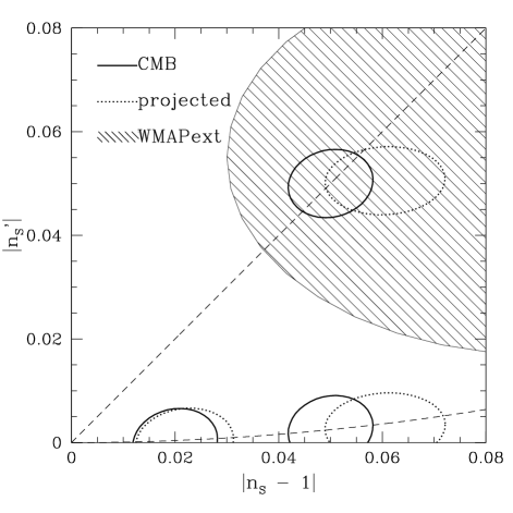
Figure 6: Solid contours show constraints in the $n_{S}$–${n_{S}}^{\prime}$ plane from the CMB data of the “CMB-pol” experiment of table 1 (using prior I-6) for scales near $k=0.0565$. Several different fiducial models are shown, two representative of the types shown in figure 1 and one large-${n_{S}}^{\prime}$ model of the type described in Dodelson and Stewart (2002). The dotted contours are the result of assuming the consistency relation of equation 7 and extrapolating from CMB scales to Lyman-$\alpha$ scales ($k=2.39$). If the relation is valid, constraints from the two types of data will be correlated in this plane as illustrated by the pairs of adjacent solid and dashed contours. All contours are drawn enclosing regions of 68% confidence level.

Table 1: Noise parameters used for simulating various experiments.

Experiment	$\sigma_{T}$	$\theta_{\mathrm{fwhm}}$	$f_{\mathrm{sky}}$	$\ell_{\textrm{max}}$
WMAP-like	20 $\mu$K	18’	0.7	1500
PLANCK-like	10 $\mu$K	6’	0.7	3000
SPT	12 $\mu$K	0.9’	0.1	4000
CMB-pol	3 $\mu$K	3’	0.7	3000

An illustration of CMB and Lyman-$\alpha$ constraints on the primordial power spectrum is shown in figures 2 and 3. If we fit a function to all the data points, and assume that function to be linear then of course the slope will be tightly constrained. If we allow the function to have a more complicated shape, the slope at any point becomes less well constrained. Figure 2 roughly represents current experimental limits. The main point of this paper is that future data can become good enough to loosen the assumptions on the shape and still produce very tight constraints. Figure 3 gives an illustration, by showing constraints on the binned power spectrum form some future experiments accurate enough to clearly distinguish a model with ${n_{S}}^{\prime}=0.05$ from a model with ${n_{S}}^{\prime}=(0.05)^{2}$, even using data spanning only one order of magnitude in wavenumber.

The ultimate limiting factor in how precise all these measurements can be is due to cosmic variance. For the CMB, the fractional error from this effect is $\Delta C_{\ell}/C_{\ell}\sim 1/\sqrt{\ell}$, which means even for large $\ell$ each individual $C_{\ell}$ can only ever be known to within a few percent. Thus the error in figure 3 is mostly cosmic variance limited, and the only way to further reduce the error is to assume some smoothness for the primordial power spectrum and bin the data. Figures 2 and 3 use a step-wise parametrization to constrain the primordial power spectrum in bins in $\ln k$, which is meaningful as long as the power spectrum is a smooth function of wavenumber relative to the bin width. For the best CMB data points, which here occur near scales corresponding to $\ell\sim 1000$, the bin width is roughly equivalent to binning a few hundred $C_{\ell}$ together.

From figure 3 we can see that the CMB accurately probes the primordial power spectrum at somewhat larger scales than those where the Lyman-$\alpha$ data is most accurate. This means the two experiments provide constraints on $n_{S}$ and ${n_{S}}^{\prime}$ at different scales, allowing us to further test our models by looking at how they predict these quantities should change with wavenumber. We will explore this idea further in section IV.

To then make error contours in the $n_{S}$–${n_{S}}^{\prime}$ plane, we use the covariance matrix from the parameter analysis to marginalize over other parameters and determine the covariance matrix for just $n_{S}$ and ${n_{S}}^{\prime}$. Of the four hypothetical CMB experiments listed in table 1, we show how well the last three place constraints in the $n_{S}$–${n_{S}}^{\prime}$ plane (for two different priors) in figures 4 and 5. We examine the fourth experiment (the best) in detail (using the weakest prior) in figure 6. These results are discussed at length in the following section. For hypothetical Lyman-$\alpha$ experiments, we do not understand the physics connecting the primordial power spectrum to measurements as well as for the CMB. We therefore “simulate” improvements in experiments as an overall reduction in statistical uncertainty due to larger samples, and an improved knowledge of the transfer function due to decreased errors in $h$, $\Omega$, and $\Omega_{b}$. For Lyman-$\alpha$ experiments to provide constraints competitive with those expected from Planck will require datasets roughly 100 times larger than current ones, and more importantly, an understanding of systematics (or at least those that affect estimates of $n_{S}$ and ${n_{S}}^{\prime}$) down to the percent level. Given that these systematics represent a lack of understanding of the (scale-dependent) light-to-mass and baryon-to-dark matter ratios, such an improvement may not appear soon. We hope to study the error for future Lyman-$\alpha$ experiments in more realistic detail in future work.

IV Testing Inflation

IV.1 Results

Table 2: Marginalized errors ($\times 1000$) in $n_{S}$ and ${n_{S}}^{\prime}$ for simulated experiments with different priors on truncating the Taylor expansion of the spectral index. Power spectrum parameters are amplitude, tilt ($n_{S}$), and for column I-$m$, the first $m$ derivatives of the tilt.

	prior I-6		prior I-3		prior I-1
Experiment	$\delta n_{S}$,	$\delta{n_{S}}^{\prime}$	$\delta n_{S}$,	$\delta{n_{S}}^{\prime}$	$\delta n_{S}$,	$\delta{n_{S}}^{\prime}$
	$(\times 1000$)		$(\times 1000$)		$(\times 1000$)
WMAP-like	309,	274	258,	152	69.1,	33.9
w polarization	203,	260	195,	132	67.8,	20.6
PLANCK-like	20.3,	13.9	16.6,	10.7	11.6,	9.79
w polarization	16.0,	10.7	12.4,	7.48	6.90,	3.94
SPT	24.6,	18.6	21.5,	14.6	16.3,	14.5
w polarization	15.2,	13.8	10.7,	8.67	6.37,	4.78
CMB-pol	9.43,	6.71	8.28,	5.67	6.17,	5.60
w polarization	5.42,	4.37	4.08,	2.42	2.32,	1.75

Table 3: Marginalized errors ($\times 1000$) in $n_{S}$ and ${n_{S}}^{\prime}$ for simulated experiments with different priors on the higher derivatives of the spectral index. Prior I-6 from Table 2 above is for reference. Priors IIa and IIb use all six derivatives in the joint parameter estimation, but IIa imposes the constraint that all higher (${n_{S}}^{\prime\prime}$ and above) derivatives are within $0.01$ of scale invariant, and IIb imposes the consistency relation (Eqn. 7) on the higher derivatives.

	prior I-6		prior IIa		prior IIb
Experiment	$\delta n_{S}$,	$\delta{n_{S}}^{\prime}$	$\delta n_{S}$,	$\delta{n_{S}}^{\prime}$	$\delta n_{S}$,	$\delta{n_{S}}^{\prime}$
	$(\times 1000$)		$(\times 1000$)		$(\times 1000$)
WMAP-like	309,	274	97.8,	38.9	70.6,	34.6
w polarization	203,	260	93.1,	34.1	69.4,	22.4
PLANCK-like	20.3,	13.9	12.3,	10.1	11.6,	9.79
w polarization	16.0,	10.7	7.50,	5.14	7.26,	4.60
SPT	24.6,	18.6	16.6,	14.5	16.5,	14.5
w polarization	15.2,	13.8	7.36,	5.19	7.00,	4.80
CMB-pol	9.43,	6.71	6.81,	5.72	6.36,	5.61
w polarization	5.42,	4.37	3.38,	2.26	3.13,	1.82

Figure 7: Constraints in the $n_{S}$–${n_{S}}^{\prime}$ plane from the Lyman-$\alpha$ data of figure 3 for scales near $k=2.39$ (thin large ovals). The projected ovals from CMB scales (dotted ovals, from Fig. 6) are then combined with the Lyman-$\alpha$ data to form improved constraints (thick small ovals). Again, 68% confidence level regions are plotted.

For completeness, we discuss a range of possible priors, each of which represents a different points of view on what one wants to take as an assumption and what one is trying to test. In tables 2 and 3 we report the constraints that various CMB experiments can place on $n_{S}$ and ${n_{S}}^{\prime}$. Our weakest prior, which we refer to as I-6, is simply to use the four cosmological parameters $(\ell_{A},\Omega_{b}h^{2},\Omega_{m}h^{2},\tau)$ and eight power spectrum parameters ($P$ and the first seven coefficients in the expansion of $n_{S}$). Having so many parameters for the power spectrum allows the shape to vary quite a bit, and loosens constraints on each term of the expansion. We include so many parameters not so much because constraints on all of them will be interesting (some, in fact, will probably always be unmeasurable), but to show the effect various assumptions about them will have on the constraints on $n_{S}$ and ${n_{S}}^{\prime}$. If the reader dislikes these parameters, our prior I-1 is equivalent to not including them at all.

To get better constraints requires either using a more restrictive prior or improving the experiment. In table 2 we change the prior by using fewer power spectrum parameters. Prior I-3 uses only the first four terms of the expansion of $n_{S}$ (i.e. up to third order), and prior I-1 uses only the first two terms, such that the only power spectrum parameters for prior I-1 are amplitude, $n_{S}$, and ${n_{S}}^{\prime}$. In table 3 we change the prior by placing a priori constraints on the higher derivative terms of the expansion, rather than dropping them completely. Prior IIa supposes that all the higher derivative terms (${n_{S}}^{\prime\prime}$ and higher) are “small”, less than $0.01$. Prior IIb also imposes the constraint that the higher derivatives be “small”, but supposes they fall off in the form of the consistency relation of equation 7.

Prior I-6 represents the weakest assumptions, and prior I-1 the tightest assumptions. (Prior I-1 basically adds just one new parameter, ${n_{S}}^{\prime}$, to the canonical set.) Prior IIb represents an assumption of the standard inflationary picture for the higher derivatives, but places no prior constraint in the $n_{S}-{n_{S}}^{\prime}$ plane so those parameters can be used to test the standard picture. (Of course, if the the standard slow roll picture fails, prior IIb may no longer be of interest)

In the time since the preprint of this paper first appeared, the WMAP collaboration announced their results Bennett et al. (2003). Our predicted error for $n_{S}$ and ${n_{S}}^{\prime}$ of 0.069 and 0.034 matches up quite well to their reported errors of 0.060 and 0.038, (using our prior I-1, which most closely matches the “WMAPext” analysis of Spergel et al. (2003).) While the WMAP results are not statistically very significant for our purposes, we plot the error contour in figure 6 for comparison. (Note that if the central value does not change much as the data improve the implications for inflation will be very interesting.)

We have simulated CMB experiments with and without polarization measurements. Since the primordial power spectrum affects the CMB temperature and polarization in exactly the same way, naively polarization simply adds a second way of measuring the same thing and should only reduce uncertainty by a factor of $\sqrt{2}$. However, allowing joint estimation of other cosmological parameters in addition to those describing the shape of the primordial power spectrum introduces confusion and near-degeneracies. The value of measuring polarization is not so much that it directly puts limits on the power spectrum, but in reducing the confusion with other parameters. Our analysis shows the increasing value of polarization as CMB experiments improve.

In figures 6 and 7 we see the error contours in the $n_{S}$–${n_{S}}^{\prime}$ plane for a hypothetical super-Planck CMB temperature and polarization experiment and for a “super” Ly-$\alpha$ survey. We see that such data would provide very significant constraints in this space. In particular, these experiments are good enough to clearly distinguish points on the line ${n_{S}}^{\prime}=n_{S}-1$ from the line ${n_{S}}^{\prime}=(n_{S}-1)^{2}$ for all but very small values of $n_{S}$, and thus would offer significant tests of the standard inflationary picture.

Combining data from both experiments will provide additional constraints and tests. Each experiment provides constraints in the $n_{S}-{n_{S}}^{\prime}$ plane, but on somewhat different scales. These amount to providing constraints on the inflaton potential $V(\phi)$ near a particular wavenumber $k$. There are several possible options for combining data from several experiments. One approach is to use a single parametrization for the primordial power spectrum and then to jointly estimate all parameters using the full dataset. If both experiments were at the same scale, this would amount to simply overlapping their individual error contours. To perform joint estimation for experiments at different scales, we would want to find parameters that are “good” across different scales, but this conflicts with our aim to test how good (i.e. constant) a parameter $n_{S}$ really is across a large range of scales. Also, a more immediate concern, is that different experiments often have a (sometimes poorly characterized) systematic error in their relative normalization which causes problems for a joint parameter analysis. For a recent discussion of these issues, see et al .

For simplicity, then, we choose a second option, which is to look at the two experiments separately and then use the consistency equation (Eqn. 7) to produce the inequality

$$\frac{n_{S}(k_{\mathrm{Ly\alpha}})-n_{S}(k_{\mathrm{CMB}})}{\ln k_{\mathrm{Ly\alpha}}-\ln k_{\mathrm{CMB}}}<(n_{S}(k_{\mathrm{Ly\alpha}})-1)^{2}$$ (20)

as an additional inflationary test. By looking at only derivatives of the power spectrum we avoid the relative normalization problems. Visually, this amounts to projecting the CMB contours for $n_{S}$ and ${n_{S}}^{\prime}$ up to Lyman-$\alpha$ scales (or vice-versa) and checking to see if the contours overlap, as shown in figure 7. This third test is not redundant because we use different pivot points ($k_{\mathrm{Ly\alpha}}$ and $k_{\mathrm{CMB}}$) for the different datasets. A potential with large higher derivatives could pass the ${n_{S}}^{\prime}<(n_{S}-1)^{2}$ test at a particular scale and yet fail it when data from different scales is used.

Finally, we would like to remind the reader that for figures 6 and 7, the real information is in the size of the error contours rather than their actual placement. In the absence of real data, we show contours from simulated data for a small sample of models all of which show correlations between the two experiments consistent with the standard inflationary picture. Ultimately nature will tell us if such correlations are really there.

IV.2 Projected errors and cross-correlations

Figure 8: Marginalized (one-sigma) errors of $n_{S}$ (solid line) and ${n_{S}}^{\prime}$ (dashed line) as a function of pixel noise and beam width. Values with(without) polarization are shown as thick(thin) lines. For the lower plot, beam width has been fixed at $6^{\prime}$, and for the upper noise has been fixed at $10\mu$K.

To further show the value of better experiments, we have investigated how the projected errors in $n_{S}$ and ${n_{S}}^{\prime}$ should change as a result of improving both resolution and noise levels. Figure 8 shows the marginalized errors (with prior I-6) with and without polarization, as functions of beam width and pixel noise.

A source of worry is possible cross-correlation between our power spectrum parameters and other cosmological parameters. Confusion between tilt and optical depth is well-known, and polarization helps greatly at reducing such confusion. We did find that there is generally a correlation between $\ell_{A}$ and our power spectrum parameters (of which ${n_{S}}^{\prime}$ is of the most interest). The correlation seems to arise because power spectrum parameters can combine to mimic a slight horizontal shift of a peak. Measuring the locations of multiple peaks makes this conspiracy of power spectrum parameters more difficult, however, and for the best experiments the correlation disappears. For the near future, an accurate determination of the angular scale of the sound horizon at last scattering will be important for placing constraints on inflationary parameters.

IV.3 The Fisher matrix approximation

One possible source of error in our calculations stems from the approximations that go into the Fisher matrix analysis technique. For low $\ell$, the covariance matrix $\mathbf{C}$ is dominated by cosmic variance, and equation 10 can be rewritten in terms of a new variable $Z_{\ell}\equiv\ln C_{\ell}$. As pointed out by Bond et. al. Bond et al. (1998), these $Z_{\ell}$ are better variables than the $C_{\ell}$ for Fisher analysis in the sense that they are Gaussian distributed. For large enough $\ell$, the difference between using $Z_{\ell}$ and $C_{\ell}$ is minor, however.

Just having variables that are Gaussian distributed is not enough; the variables should respond linearly to the parameters. Linearity in response to the cosmological parameters is a well-studied problem and has been discussed extensively in the literature (see Kosowsky et al. (2002) for a recent discussion). What remains is to check our power spectrum parameters. We have done this by examining $Z_{\ell}$ as a function of the power spectrum parameters.

For the power spectrum parameters we are most interested in ($n_{S}$ and ${n_{S}}^{\prime}$), deviations from linearity are less than one percent for parameter values within all the errorbars that we report in tables 2 and 3. For the higher order parameters, the worst deviations from linearity occur only for small $\ell$ ($\sim 10$), for which we found the linear approximation to be valid within one percent for parameter values less than around 0.02. In our calculations, we varied the higher order parameters by amounts several times smaller than this, and while the resulting errorbars were sometimes larger than this, at these small $\ell$ the error from cosmic variance is also large, so the effect on the overall parameter analysis is small. We checked this by redoing the parameter analysis without including low $\ell$ values at all, and the qualitative results of our work do not change. For higher $\ell$ ($\sim 200$ and above), the linear approximation remains good up to parameter values of order unity.

V Conclusion

We have shown that the next generation of cosmological experiments should determine the shape of the primordial power spectrum sufficiently to allow new tests of the the standard picture of inflation. If the standard picture is upheld, a new level of differentiation among different inflaton potentials will be possible. We have investigated the potential impact of new data on both the CMB and the Lyman-$\alpha$ forest.

The Lyman-$\alpha$ data offers a promising route to testing slow-roll models both on its own, and in conjunction with CMB data. Currently published data does not get too far with this enterprise, but next-generation observation could have considerable impact.

For the CMB data, if we are interested in general constraints without placing restrictive priors on the primordial power spectrum, Planck-like CMB experiments do not quite have the precision to put the strong limits on ${n_{S}}^{\prime}$ that we desire. It is not until relatively high $\ell$ that the uncertainty from cosmological variance is low enough for our requirements, and it is precisely at these high $\ell$ that the Planck experiment noise rapidly becomes dominant so a further improvement beyond Planck is needed. Our hypothetical “CMB-pol” experiment should start placing interesting constraints in the $n_{S}$–${n_{S}}^{\prime}$ plane. Also important is the measurement of the (E-mode) polarization channel, which is vital to reducing degeneracies that make the tests more challenging.

For constraints on the power spectrum itself (as opposed to other cosmological parameters), information from low multipole moments ($\ell<500$) contributes very little due to cosmic variance. However, coverage of a reasonable fraction of the sky is needed to retain high resolution in $\ell$, and simply to beat down statistical noise. The proposed South Pole Telescope (SPT) may do well in this regard. Higher multipole moments are useful up until Silk damping reduces the overall CMB signal. As CMB experiments improve, polarization will become more important as the key to breaking degeneracies between the effects of the power spectrum shape, which affects temperature and polarization identically, and other cosmological parameters, which generally do not.

Appendix A Models

The potentials used in the models shown in figure 1, from left to right are (in units where $M_{P}\equiv 1$)

$$M^{4}\left[1+A\ln\phi\right],$$ (21)

$$M^{4}\left[1-e^{-\phi/2}\right]^{2},$$ (22)

$$M^{4}\left[1-e^{-\phi}\right],$$ (23)

$$M^{4}\left[1+A\phi^{2}\right],$$ (24)

$$M^{4}\cos^{2}\frac{\phi}{A},$$ (25)

$$M^{4}\left[1-A\phi^{12}\right],$$ (26)

$$M^{4}\left[1-A\phi^{2}\right],$$ (27)

$$M^{4}\left[1-A\phi^{4}\right],$$ (28)

$$M^{4}\left[1+\frac{1}{2}\phi^{2}\left(A+0.6\right)\right].$$ (29)

In all cases the mass scale and other parameters were chosen as in table 4 to produce a $\delta\rho/\rho$ of roughly $2\times 10^{-5}$.

Table 4: Inflationary model parameters

Model #	$M$	$A$
1	$10^{-3}$	$5\times 10^{-2}$
2	$10^{-3}$	—
3	$10^{-3}$	—
4	$10^{-4}$	$10^{-3}$
5	$10^{-9/4}$	$100$
6	$2\times 10^{-4}$	$5\times 10^{-3}$
7	$10^{-3}$	$10^{-2}$
8	$10^{-6}$	$\frac{1}{4}\times 10^{9}$
9	$10^{-16}$	$0.139$

References

- Copeland et al. (1993) E. Copeland, E. W. Kolb, A. R. Liddle, and J. E. Lidsey, Phys. Rev. D 48, 2529 (1993).
- Knox (1995) L. Knox, Phys. Rev. D 52, 4307 (1995).
- Kosowsky and Turner (1995) A. Kosowsky and M. S. Turner, Phys. Rev. D 52, 1739 (1995).
- Jungman et al. (1996) G. Jungman, M. Kamionkowski, A. Kosowsky, and D. N. Spergel, Phys. Rev. D 54, 1332 (1996).
- Copeland et al. (1998) E. J. Copeland, I. J. Grivell, and A. R. Liddle, Mon. Not. Roy. Astron. Soc. 298, 1233 (1998).
- Dodelson et al. (1997) S. Dodelson, W. H. Kinney, and E. W. Kolb, Phys. Rev. D 56, 3207 (1997).
- Kinney et al. (2001) W. H. Kinney, A. Melchiorri, and A. Riotto, Phys. Rev. D 63, 023505 (2001).
- Hannestad et al. (2002) S. Hannestad, S. H. Hansen, F. L. Villante, and A. J. S. Hamilton, Astroparticle Physics 17, 375 (2002).
- Hansen and Kunz (2002) S. H. Hansen and M. Kunz, Mon. Not. Roy. Astron. Soc. 336, 1007 (2002), eprint hep-ph/0109252.
- Bucher et al. (2000) M. Bucher, K. Moodley, and N. Turok (2000), eprint astro-ph/0011025.
- Guth (1981) A. H. Guth, Phys. Rev. D 23, 347 (1981).
- Albrecht and Steinhardt (1982) A. Albrecht and P. Steinhardt, Phys. Rev. Lett. 48, 1220 (1982).
- Linde (1982) A. D. Linde, Phys. Lett. B 108, 389 (1982).
- Linde (1983) A. D. Linde, Phys. Lett. B 129, 177 (1983).
- Bardeen (1980) J. M. Bardeen, Phys. Rev. D 22, 1882 (1980).
- Dodelson and Stewart (2002) S. Dodelson and E. Stewart, Phys. Rev. D65, 101301 (2002), eprint astro-ph/0109354.
- Tegmark and Zaldarriaga (2002) M. Tegmark and M. Zaldarriaga, Phys. Rev. D 66, 103508 (2002).
- (18) D. H. Lyth, eprint hep-ph/9609431.
- Liddle and Lyth (2000) A. R. Liddle and D. H. Lyth, Cosmological Inflation and Large-Scale Structure (Cambridge University Press, 2000).
- Dvali and Tye (1999) G. Dvali and S.-H. H. Tye, Phys. Lett. B 450, 72 (1999).
- Guth and Pi (1982) A. H. Guth and S.-Y. Pi, Physical Review Letters 49, 1110 (1982).
- Shiu and Tye (2001) G. Shiu and S.-H. H. Tye, Phys. Lett. B 516, 421 (2001).
- Covi et al. (2003) L. Covi, D. H. Lyth, and A. Melchiorri, Phys. Rev. D 67, 43507 (2003).
- Croft et al. (2002) R. A. C. Croft, D. H. Weinberg, M. Bolte, S. Burles, L. Hernquist, N. Katz, D. Kirkman, and D. Tytler, Astrophys. J. 581, 20 (2002).
- Wang et al. (1999) Y. Wang, D. N. Spergel, and M. A. Strauss, Astrophys. J. 20, 510 (1999).
- Zaldarriaga and Seljak (1996) M. Zaldarriaga and U. Seljak, Astrophys. J. 469, 437 (1996).
- Zaldarriaga and Seljak (1997) M. Zaldarriaga and U. Seljak, Phys. Rev. D55, 1830 (1997), eprint astro-ph/9609170.
- Knox et al. (2002) L. Knox, C. Skordis, and M. Kaplinghat, Astrophys. J. 578, 665 (2002), eprint astro-ph/0203413.
- Peacock and Dodds (1994) J. A. Peacock and S. J. Dodds, Mon. Not. R. Astron. Soc. 267, 1020 (1994).
- Bennett et al. (2003) C. L. Bennett et al., Astrophys. J. (2003).
- Spergel et al. (2003) D. N. Spergel et al., Astrophys. J. (2003).
- (32) K. et al, Proceedings of the davis meeting on cosmic inflation, eprint astro-ph/0304225.
- Bond et al. (1998) J. R. Bond, A. H. Jaffe, and L. Knox, Phys. Rev. D 57, 2117 (1998).
- Kosowsky et al. (2002) A. Kosowsky, M. Milosavljevic, and R. Jimenez, Phys. Rev. D 66, 63007 (2002).
- Hu (2003) W. Hu, Annals of Physics 303, 203 (2003).
- Seljak (2002) U. Seljak, Private communication (2002).