Mapping Magnetic Fields in the Cold Dust at the Galactic Center

Abstract

We report the detection of polarized emission in the vicinity of the Galactic center for 158 positions within eight different pointings of the Hertz polarimeter operating on the Caltech Submillimeter Observatory. These pointings include positions 2′  offset to the E, NE, and NW of M-0.02-0.07; positions to the SE and NW of the 20 km s^-1 cloud (M-0.13-0.08), CO+0.02-0.02, M+0.07-0.08, and M+0.11-0.08. We use these data in conjunction with previous far-infrared and submillimeter polarization results to find that the direction of the inferred magnetic field is related to the density of the molecular material in the following way: in denser regions, the field is generally parallel to the Galactic plane, whereas in regions with lower densities, the field is generally perpendicular to the plane. This finding is consistent with a model in which an initially poloidal field has been sheared into a toroidal configuration in regions that are dense enough such that the gravitational energy density is greater than the energy density of the magnetic field. Using this model, we estimate the characteristic strength of the magnetic field in the central 30 pc of our Galaxy to be a few mG.

1 Introduction

Despite significant advancement over the last two decades, the Galactic center magnetosphere is still not well understood; however, determining the geometry and strength of the magnetic field in this region is crucial to developing an understanding of the dynamics of the Galactic center. One reason that the magnetosphere is of interest lies in the Galactic center’s role as an Active Galactic Nucleus. In the central engines of galaxies, magnetic fields are believed to be important in angular momentum transport and jet dynamics.

The most striking evidence for the existence of magnetic fields in the Galactic center is the existence of the Non-thermal Filaments (NTFs) of the Galactic center Radio Arc (GCRA) (Yusef-Zadeh et al., 1984). Radio polarization measurements have confirmed the synchrotron nature of the emission from these filaments and support the notion that the filaments trace magnetic field lines (Tsuboi et al., 1986). Almost all of the confirmed NTFs that have been discovered in the Galactic center region are aligned with their long axes within 20^∘ of perpendicular to the plane of the Galaxy (LaRosa et al., 2000). The presence of these filaments has led to the idea that these filaments trace the inner part of a dipole or poloidal magnetic field.

In many cases NTFs are observed to be interacting with Galactic center molecular clouds. The best example of this is in the center of the GCRA where the 25 km s^-1 molecular cloud associated with G0.18-0.04 (the Sickle) is coincident with the filaments (Serabyn & Güsten, 1991). The lack of observed distortion of the filaments allows one to set a lower limit for the strength of the magnetic field. This argument yields $B>{\mathrm{few\,mG}}$ (Yusef-Zadeh & Morris, 1987). The association of molecular clouds with NTFs gives additional evidence for the dynamical importance of these fields and has motivated the idea that the generation of the relativistic electrons required to create these NTFs could occur as a result of a molecular cloud/magnetic flux tube interaction. The specific mechanism thought to be responsible for the generation of these relativistic electrons is magnetic reconnection between the fields in the flux tube and those in the cloud (Serabyn & Morris (1994); for a review, see Davidson (1996)).

Magnetically aligned dust grains are known to emit polarized radiation in the far-infrared and submillimeter. Thus, polarimetry at these wavelengths has proven to be a reliable technique for measuring the projected, line-of-sight integrated magnetic field configuration. Previous polarimetry data have shown that the field in the dense molecular clouds is not generally consistent with the poloidal field traced by the filaments. Novak et al. (2000) have shown that in the molecular cloud M-0.13-0.08, the field is nearly parallel to the Galactic plane, indicating that gravitational rotation and infall have sheared out the field into a toroidal configuration. In addition, 60 $\mu$m polarimetry of the molecular cloud associated with the Sickle indicates that the field in this region is parallel to the Galactic plane (Dotson et al., 2000).

Uchida et al. (1985) have constructed a model that connects poloidal and toroidal fields. Because the magnetic flux is frozen into the matter, differential rotation and infall can shear an initially poloidal field into a toroidal one in sufficiently dense regions of the Galactic center. Novak et al. (2002) have shown that on large scales, the dust in the Central Molecular Zone (CMZ) of the Galaxy is permeated by a field that is oriented in a direction parallel to the plane of the Galaxy. They compare their observation to the spatial distribution of the direction of Faraday rotation in the Galactic center and show that these two different techniques for sampling fields yield results that are consistent with such a model.

We extend the ideas that underlie the above model to the inner 30 parsecs of the Galactic center. When resolved with sub-arcminute resolution in the submillmeter (Pierce-Price et al., 2000), this region exhibits a clumpiness resulting from spatial density variations. We find that in less dense regions, the magnetic field that permeates the dust is poloidal, consistent with that found in the filaments. In these regions, the matter density is too low for gravity to shear the field into a toroidal configuration. In the dense molecular clouds, however, the field appears to be generally toroidal, indicating that in such regions, the energy density of gravity dominates that of the permeating magnetic field.

Section 2 describes the observations. In section 3, the data are discussed. Finally, conclusions are presented in section 4.

2 Observations

The data were obtained using the University of Chicago 32-pixel polarimeter, Hertz (Dowell et al., 1998) at the Caltech Submillimeter Observatory on Mauna Kea, Hawai’i in April of 2001. The beam size of Hertz is 20″ FWHM with a pixel spacing of 18″. The central wavelength of the Hertz passband is 350 $\mu$m with a $\Delta\lambda\over\lambda$ of 0.1.

The observing technique used with Hertz involves a combination of high frequency “chopping” in which the array footprint is alternately pointed at the source and a reference position 6′  away in cross-elevation and low frequency “nodding” during which the source is alternately placed in the right and left beams of the telescope. One undesirable complication that this observational scheme introduces is the problem of polarized flux in the reference beam. This problem is discussed in detail in § 3.4.

For a full description of the observing and analysis procedures see Schleuning et al. (1997) and Dowell et al. (1998).

During the observations, a total of 158 new polarization measurements were obtained having a polarimetric signal-to-noise greater than 3. These data are given in Tables 1 through 7.

3 Discussion

3.1 Morphology of the Inner 30 Parsecs

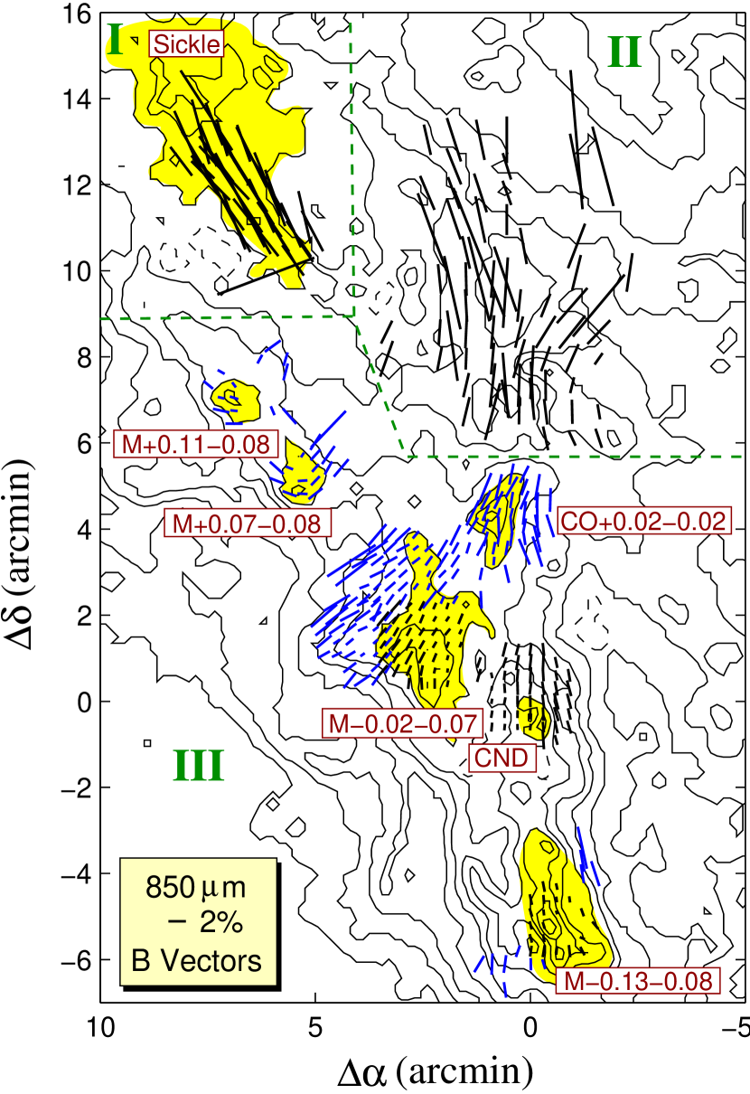
Figure 1: The inferred magnetic field directions for polarization measurements in the Galactic center are displayed on 850 $\mu$m contours from SCUBA/JCMT (Pierce-Price et al., 2000). Region I shows 60 $\mu$m polarimetery of the Sickle (Dotson et al., 2000). Region II shows 100 $\mu$m polarimetry of the Arched Filaments (Dotson et al., 2000). Region III shows new 350 $\mu$m inferred magnetic field vectors along with the 350 $\mu$m vectors from Novak et al. (2000). Important dust features are shaded and labeled. The axes scales are offsets in arcminutes from the position of Sgr A* ($\alpha_{2000}=17^{\mathrm{h}}45^{\mathrm{m}}40\fs 04$, $\delta_{2000}=-29^{\circ}00^{\prime}28\farcs 07$).

The magnetic field vectors inferred from these data are shown in blue in region III of Figure 1. The black vectors in this region are those from Novak et al. (2000). Also shown in this figure are 100 $\mu$m data from the Kuiper Airborne Observatory (Dotson et al., 2000) of the Arched Filaments (region II) and 60 $\mu$m data (Dotson et al., 2000) of the Sickle (region I). The 100 $\mu$m and 50 $\mu$m data have beam sizes of 35$\arcsec$ and 22$\arcsec$, respectively. The contours trace 850 $\mu$m flux (Pierce-Price et al., 2000). Major molecular features are labeled.

3.1.1 M-0.13-0.08

The molecular cloud M-0.13-0.08 (commonly called the 20 km s^-1 cloud) has an elongated shape, and its long axis is oriented at a shallow (15^∘) angle to the Galactic plane (See Fig. 1). The cloud is thought to be located in front of the Galactic center since it appears in absorption in the mid-infrared (Price et al., 2001). In projection, the long axis of this cloud points in the direction of Sgr A*. This fact suggests that this cloud is undergoing a gravitational shear as it falls toward Sgr A*. This is supported by other observations including a high velocity gradient along the long axis (Zylka et al., 1990), increasing line widths and temperatures along the cloud in the direction of Sgr A* (Okumura et al., 1991), and an extension of the cloud detected in NH₃ emission to within 30^′′ of Sgr A* in projection (Ho et al., 1991). Novak et al. (2000) have discovered that the magnetic field structure is such that the field is parallel to the long axis of the cloud. They point out that for gravitationally sheared clouds, a consequence of flux-freezing is that regardless of the initial configuration of the field, the field will be forced into a configuration in which it is parallel to the long axis of the cloud. In addition, these authors note that this is not only true for the dense material inside of the cloud, but also for the more diffuse molecular material that belongs to the ambient region. They note that the southern end of this cloud exhibits a flare both morphologically and in magnetic field structure. They suggest that this flare is a connection to the large scale poloidal field traced by the NTFs.

Our 7 new vectors in this region provide additional support for this interpretation, but a more extensive polarimetric mapping of this cloud is necessary before a complete interpretation is made.

3.1.2 G0.18-0.04

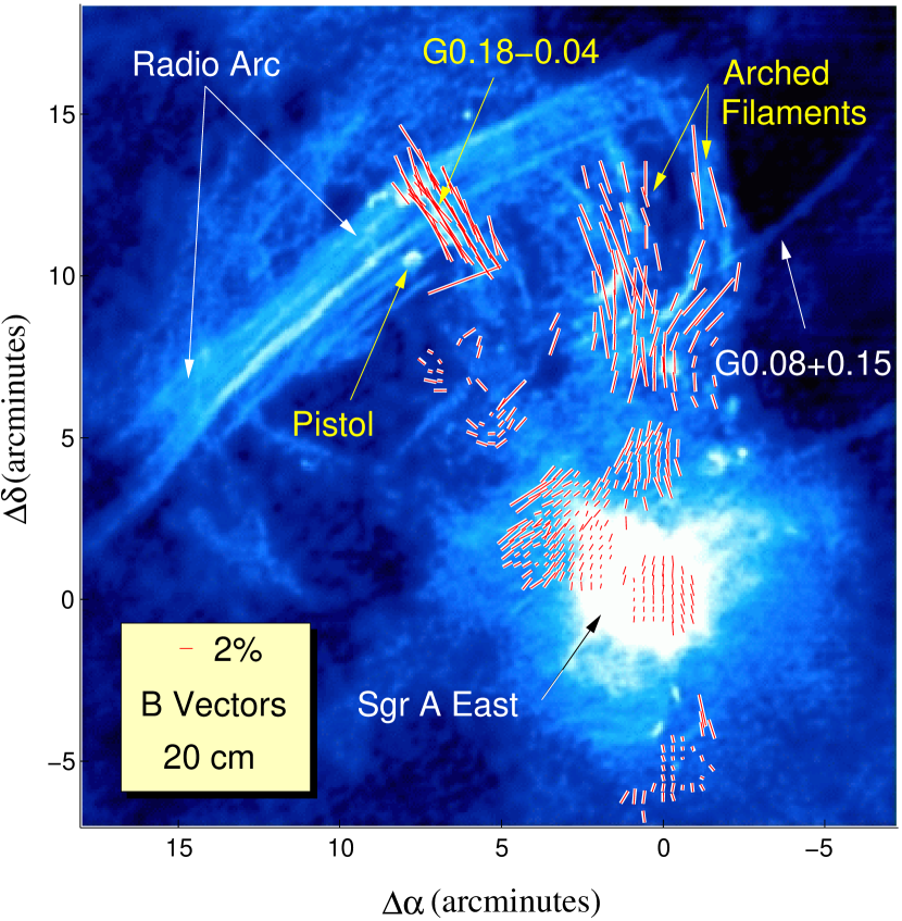
Figure 2: Inferred B vectors are superposed on a 20 cm map (Yusef-Zadeh et al., 1984) taken with the VLA. Important thermal and non-thermal structures are labeled in yellow and white, respectively. The 100 $\mu$m vectors appear to trace the Arched Filaments. The field in the molecular cloud associated with G0.18-0.04 is perpendicular to the field associated with the Radio Arc.

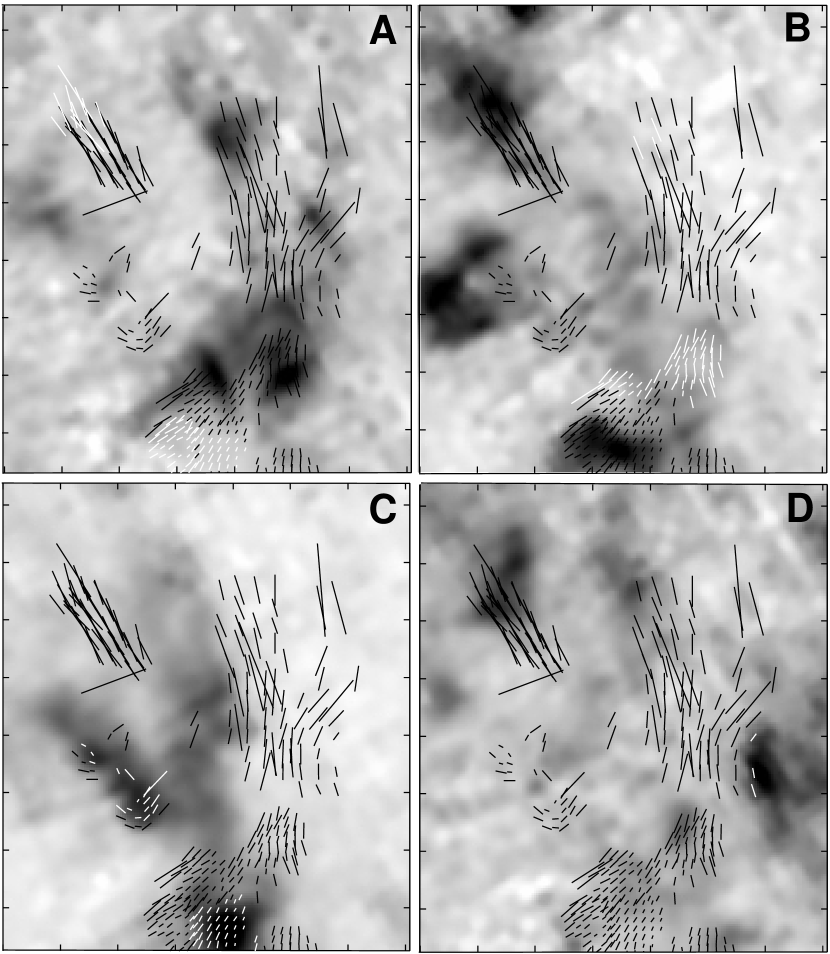
Figure 3: CS maps (Tsuboi et al., 1997) are shown with polarization data superposed. Panel A shows structures at $\sim$-15 km s^-1, the most prominent of which is the molecular material associated with the arched filaments. Panel B shows material at $\sim$30 km s^-1. The molecular material associated with the Sickle ($v\sim 25$ km s^-1) is visible here. Panel C shows material at $\sim$50 km s^-1. M+0.11-0.08, M0.07-0.08, and M-0.02-0.07 are all prominent at this velocity. Note that the magnetic field vectors at the southwestern edge of M0.07-0.08 trace the edge of the cloud indicating that the cloud has a velocity in the plane of the sky that is directed toward M-0.02-0.07, a region of predominantly poloidal flux. Panel D traces $\sim$85 km s^-1 material. Note the edge of the cloud in the lower right of the panel seems to be traced by the 100 $\mu$m magnetic field vectors.

The H II region G0.18-0.04 (commonly called the “Sickle”) can be seen in 20 cm thermal emission in Figure 2. It is believed to be the ionized surface of a molecular cloud that is interacting with the Radio Arc (Serabyn & Güsten, 1991). Its molecular counterpart can be seen in Figure 3B. It has been suggested that this interaction is responsible for producing the relativistic electrons necessary to light up the Radio Arc via magnetic reconnection (Serabyn & Güsten, 1991; Davidson, 1996).

The relationship between the geometry of the cloud and its magnetic field structure is similar to that of M-0.13-0.08. The cloud is elongated parallel to the plane of the Galaxy and its magnetic field as inferred from far-infrared polarimetry is parallel to the long axis. These similarities to M-0.13-0.08 suggest a similar origin of the field geometry.

One difference between this cloud and M-0.13-0.08 is that in the case of the former there is no observed flaring of the field. In fact, the stark 90^∘ difference between the toroidal field observed in the molecular material and the pristine poloidal geometry of the superposed Radio Arc suggest that there is little connection between the toroidal field and the poloidal field in this vicinity. There are several possibilities for why this might be the case. First, the polarimetry coverage may be too limited in this region. More data taken in surrounding region may reveal a connection to a poloidal field. Second, this cloud may be more evolved than M-0.13-0.08, and so we may be observing a magnetic field that has had enough time to shear into a more parallel configuration than that of M-0.13-0.08. Finally, because this molecular cloud is farther from the dynamical center of the Galaxy than is M-0.13-0.08, the tidal forces on it are weaker, thus allowing for a more uniform shearing along its length.

3.1.3 M+0.11-0.08 and M+0.07-0.08

M+0.11-0.08 and M+0.07-0.08 are two peaks of a molecular cloud complex that, like M-0.13-0.08 and the molecular cloud associated with the Sickle, is elongated nearly parallel to the plane with its long axis pointed toward Sgr A*. The radial velocity of this complex has been measured to be $\sim$50 km s^-1 (see Fig. 3C).

The inferred magnetic field configuration for this complex displays a geometry that is quite unique. The field appears to tightly wrap around the southern and eastern edges of this cloud. The implication of this curvature of the magnetic field is that the cloud is moving toward the Sgr A* region in projection and is sweeping up magnetic flux from the intercloud medium. The direction of travel inferred from the polarization data indicates that in projection, this cloud is moving toward a region dominated by a poloidal field (see northeast side of M-0.02-0.07 in Fig. 1). As the cloud moves through the less dense intercloud medium, this poloidal flux then is wrapped around the cloud into a toroidal configuration as seen along the eastern edge of the cloud. The result is an observed transition between poloidal and toroidal fields.

Interior to this cloud complex, there are few measurements; however, those that exist hint at a field that is parallel to its long axis, similar to that of M-0.13-0.08 and the molecular cloud associated with the Sickle.

3.1.4 The X Polarization Feature

The 350 $\mu$m polarimetric observations of M-0.02-0.07, the CND, and CO+0.02-0.02 provide evidence for a magnetic field structure that is contiguous with that derived from the 100 $\mu$m polarimetric observations of the Arched Filaments to form an “X-shaped” feature that we will refer to as the “X Polarization Feature.” The feature extends (in the coordinate system of Fig. 1) from (-1, 13) down through (5, 0). The organization of the magnetic field vectors appears to be on scales (30 pc) significantly larger than those of typical Galactic center molecular clouds (5-10 pc). This fact reinforces the notion that the vectors trace a single global field that is subject to environmental forces.

It is likely that the X Polarization Feature is a line-of-sight superposition of regions of poloidal and toroidal fields. The orientation of the observed magnetic field at any given location depends on the relative polarized emission from poloidal and toroidal regions that intersect the line of sight. For example, the poloidal field is seen to dominate in the eastern part of the M-0.02-0.07 cloud and at the western edge of the Arched Filaments. The toroidal field dominates at the eastern edge of the Arched Filaments and around the CND. The two fields mix in CO+0.02-0.02.

Another example of line-of-sight mixing of poloidal and toroidal fields occurs at the western edge of the Arched Filaments. Here, there exist several magnetic field vectors oriented perpendicular to the plane that are in close proximity to the G0.08+0.15, a NTF that traces the poloidal field. Just to the north, the magnetic field vectors return quite abruptly to a toroidal configuration in the vicinity of the molecular features that correspond to the Arched Filaments. It is possible that the molecular material at $v\sim-15$ km s^-1 (See Fig. 3A) is displaced along the line of sight from G0.08+0.15, and the net polarization observed consists of contributions from dust associated with the respective neighborhoods of these two features. To the south of G0.08+0.15, the vectors again become indicative of a field distorted by gravity as they wrap around the molecular cloud visible in Figure 3D.

3.2 Polarized Flux

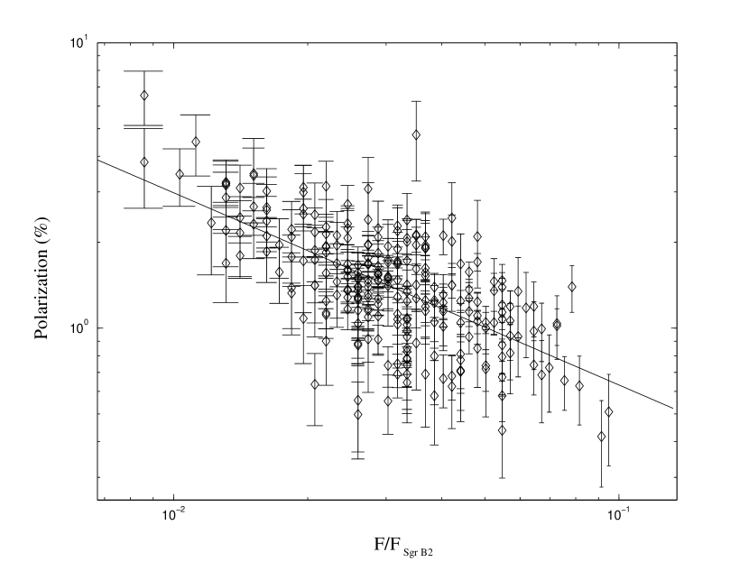
Figure 4: 350 µm  polarization is plotted against 350 µm  flux. The cutoff for these data is 3 $\sigma$ and the data have been corrected by $P^{\prime}=\sqrt{P^{2}-\sigma_{P}^{2}}$ (Serkowski, 1974). The best fit slope of this curve is -0.67.

Figure 4 shows the relationship between Galactic center polarization measured by Hertz versus the 350 $\mu$m flux measured by SHARC, a 350 $\mu$m photometer with a 15$\arcsec$ beam (Dowell et al., 1999). A linear fit gives a slope of -0.67. In this plot, we have included all points with a polarization signal-to-noise (S/N) greater than 3 and have corrected the polarization by $P^{\prime}=\sqrt{P^{2}-\sigma_{P}^{2}}$ in order to account for the systematic overestimation of polarization (Serkowski, 1974) inherent in the conversion from $q$ and $u$ to $P$ and $\phi$. Figure 4 shows a depolarization effect associated with an increase in 350 $\mu$m flux.

Because of a concern over a selection effect that systematically excludes low polarizations at low fluxes, the test was repeated with a S/N cutoff of 1. For this case, the slope decreases to -0.73, thus exonerating Figure 4 of this effect. The test was repeated for the 11 individual Hertz pointing corresponding to both this work and that of Novak et al. (2000). A polarization versus flux comparison using the relative fluxes obtained simultaneously with the polarizations gives an average slope of -0.96$\pm$0.32. This number is the mean of the slopes for each of the 11 fields. The error is the standard deviation of these slopes.

These numbers are similar to the values found by Matthews et al. (2001, 2002) for various Galactic molecular clouds. Matthews et al. (2002) suggest three possibilities for the depolarization effect (see also Schleuning (1988) and Dotson (1986)). First, the lower polarization could be due to poor grain alignment or low polarization efficiency in the cores of these clouds. Second, the depolarization could be a result of a geometrical cancellation of the front and back of a three dimensional field that is threaded through the optically thin cloud. Finally, it is possible that the spatial structure of the magnetic fields in the cores of clouds is too small to be resolved by Hertz’s beam.

The evidence for depolarization in the Galactic center does not provide enough information to differentiate among the three proposed explanations; however, it does indicate that the depolarization effect is observable in clouds that are a factor of $\sim$10 larger than molecular clouds in the disk of the Galaxy.

3.3 Strength of the Magnetic Field

Historically the lack of information concerning the degree of grain alignment and relative strength of the line-of-sight component of the magnetic field have limited the ability of far-infrared and submillimeter polarimetry to provide information concerning the strengths of magnetic fields. We will show that in the Galactic center the additional information concerning magnetic fields (i.e. the NTFs) can lead to a model-based estimate of a characteristic global magnetic field strength estimate.

In studying the magnetic field in the central 30 pc of the Galaxy, we revisit the model of Uchida et al. (1985) as it applies to the Galactic center. Specifically, we keep in mind that the Galactic center is clumpy and that some regions seem to contain a field that is poloidal while others contain a field that is toroidal. In the spirit of this model, we adopt a picture in which gravity is assumed to dominate the dynamics in regions of toroidal fields. Conversely, in regions of poloidal fields, magnetic fields are assumed to be energetically dominant.

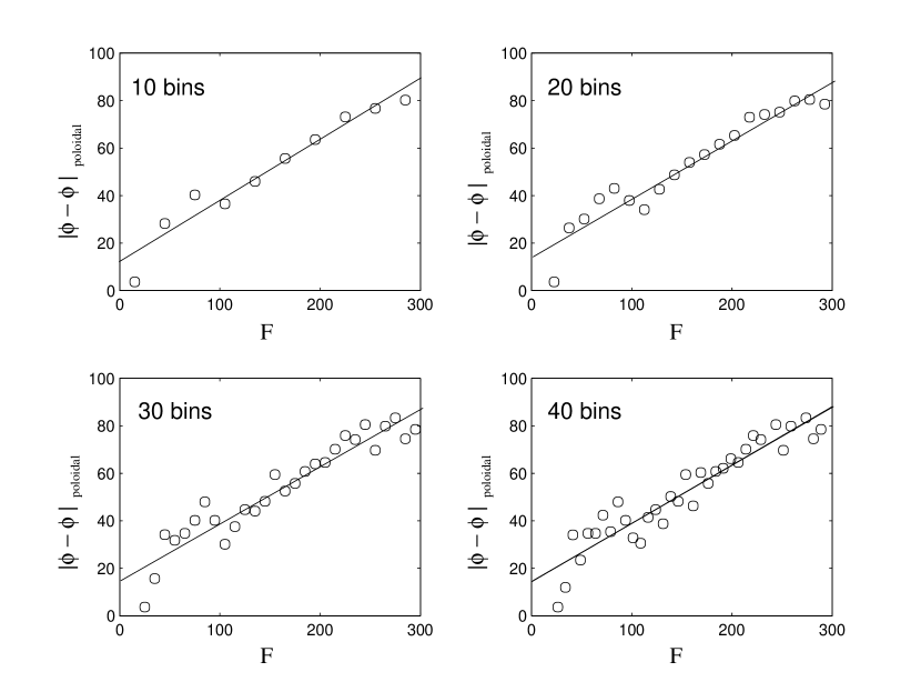
Figure 6: The fluxes are grouped into bins, and the mean of polarization angle in each bin is plotted against the mean flux in each bin. For each binning, the flux for equality of magnetic and gravitational forces has been calculated by fitting a line and then determining the flux value for a 45^∘ deviation from a poloidal field. By taking the average of the flux values for each of the 4 plots, this flux is 125 Jy beam^-1. The error in the choice of bin size is $\sim$ 1 Jy beam^-1.

Figure 5 illustrates the dependence of the polarization angle on the flux measured by SHARC (Dowell et al., 1999). In this figure, the absolute deviation from a poloidal field ($|\phi-\phi_{\mathrm{poloidal}}|$) is plotted against 350 $\mu$m flux. This relationship shows that for regions having higher flux (and thus higher column densities), the field is toroidal and the dynamics are gravity-dominated. For lower intensities, poloidal fields are observed indicating that there are regions of low density in which the dynamics are dominated by the energy density associated with the magnetic field. Somewhere between these two extremes is a flux for which the energy density of the poloidal field equals that of the gravitational energy density. In order to proceed with the estimate, we will assume that this density corresponds to a measured angle $|\phi-\phi_{\mathrm{poloidal}}|=45^{\circ}$. This choice is somewhat arbitrary. In order to find the flux corresponding to this angle, we perform various binnings as shown in Figure 6. Linear fits to each of these four plots give a flux of 125 Jy beam^-1. To a crude approximation, this energy balance condition is represented by

$$\frac{1}{2}\rho v^{2}=\frac{B^{2}}{8\pi}.$$ (1)

Here, the kinetic energy density of material orbiting in the gravitational potential well of the Galaxy is equated to the magnetic energy density.

The key to this problem now becomes the estimate of $\rho$ and $v$. The velocity, $v$, can be estimated from typical cloud velocities (Tsuboi et al., 1999) and is expected to be between $50-150$ km s^-1. The density can be determined as follows.

The brightness one observes from a thermal source having an optical depth $\tau_{\nu}$ is

$$I_{\nu}=B_{\nu}(T)(1-\mathrm{e}^{-\tau_{\nu}}),$$ (2)

where $B_{\nu}(T)$ is the Planck function.

In the case of 350 $\mu$m observations, the optical depth is generally small. For $\tau_{\nu}\ll 1$,

$$I_{\nu}=\tau_{\nu}B_{\nu}(T).$$ (3)

SHARC measures $F_{\nu}=I_{\nu}\Delta\Omega$, the flux of the incoming radiation where $\Delta\Omega$ is the solid angle subtended by a SHARC array element. From these equations, it is possible to express the optical depth of the dust as a function of temperature and measured flux.

$$\tau_{\nu}=\frac{F_{\nu}}{B_{\nu}(T)\,\Delta\Omega}$$ (4)

Alternatively, we can express the optical depth as a function of grain properties along the line of sight. Once again we are working in the limit $\tau_{\nu}\ll 1$. We can imagine a column of dust along the line of sight that extends through the entire depth of the Galactic center. The optical depth is proportional to the number density of dust grains along the line of sight ($N_{d}$). It is also proportional to the typical geometrical cross-section of each of the grains ($\sigma_{d}$); however, since the grain sizes are generally much smaller than the wavelenth of the radiation, the efficiencies of the grains for emitting, scattering or absorbing light are much lower than this blackbody approximation indicates. Thus we write the optical depth as

$$\tau_{\nu}=N_{d}\,Q_{e}\,\sigma_{d},$$ (5)

where $Q_{e}$ is the emissivity of the dust grains and is generally much less than unity for submillimeter radiation.

Once the $N_{d}$ is found, the total dust mass observed by a SHARC beam is

$$M_{d}=N_{d}\,\rho_{d}\,v_{d}\,\Delta\Omega\,D^{2}.$$ (6)

Here, $D$ is the distance to the source and $\Delta\Omega D^{2}$ is simply the physical size of SHARC’s beam at a distance $D$. $\rho_{d}$ and $v_{d}\sim\frac{4}{3}\pi a^{3}$ are the density and volume of a dust grain, respectively. If we then make the appropriate substitutions and assume a gas-to-dust ratio, $X\gg 1$, we get the following expression for the total mass.

$$M=\frac{4\,F_{\nu}\,\rho_{d}\,a\,D^{2}X}{3\,Q_{e}\,B_{\nu}(T)}$$ (7)

Putting in the appropriate numbers for 350 $\mu$m radiation yields

$$\frac{M}{M_{\odot}}=\left({\frac{F}{\mathrm{Jy}}}\right)\left({\frac{\rho_{d}}{\mathrm{g\,cm^{-3}}}}\right)\left({\frac{a}{\mu\mathrm{m}}}\right)\left({\frac{D}{\mathrm{kpc}}}\right)\\ \left({\frac{X}{Q_{e}}}\right)6.89\times 10^{-7}(\mathrm{e}^{41.1/T}-1).$$ (8)

The density can be calculated by assuming a value for the depth of the dust layer ($L$).

$$\rho=\frac{M}{\Delta\Omega^{2}\,D^{2}\,L}$$ (9)

We use the following grain properties (Dowell et al., 1999) for our grain model. These are $a=0.1\,\mu\mathrm{m}$, $Q_{e}=1.9\times 10^{-4}$, $X=100$, and $\rho_{d}=3\,\mathrm{g\,cm^{-3}}$. In addition, Pierce-Price, et al. (2000) have used SCUBA to map the Central Molecular Zone (CMZ) at 450 and 850 $\mu$m. They have found the dust temperature to be relatively uniform over the CMZ and adopt a value of 20 K. With these numbers, one can get an estimate of the magnetic field strength as a function of velocity of the material and the thickness of the dust.

$$B=3\,\mathrm{mG}\left({\frac{L}{200\,\mathrm{pc}}}\right)^{-\frac{1}{2}}\left({\frac{v}{100\,\mathrm{km\,s^{-1}}}}\right)$$ (10)

Based on CS measurements of the CMZ (Tsuboi et al., 1999), most molecular material has v $<$ 150 km s^-1. The CMZ has a projected diameter of 200 pc. Assuming cylindrical symmetry, this is approximately the scale of the material along the line of sight.

Because of the clumpy nature of the central 30 pc, this value $L$ is most likely overestimated, thereby making the above estimate of $B$ conservatively low.

3.4 Reference Beam Contamination

In performing differential measurements using chopping techniques, polarized flux in the reference beam positions is always a potential hazard. Because of the extended nature of the dust in the Galactic center, it is of particular importance to understand the possible effect of reference beam contamination on the data presented here. Several attempts have been made to quantify this issue (Novak et al., 1997; Schleuning et al., 1997; Matthews et al., 2001). The goal of this section is to assess the level of reference beam contamination in our data. Note that throughout this analysis quantities pertaining to the “reference beam” such as $P_{\mathrm{r}}$ and $I_{\mathrm{r}}$ refer to the average of these quantities over the multiple reference beam positions used in the observations.

Since the quantitative result of this work centers on the relationship shown in Figure 5, we are concerned primarily with the polarization angle ($\phi$), and so we wish to estimate the maximum effect of polarized flux in the reference beam on $\phi$. The difference between the source polarization angle ($\Phi_{\mathrm{s}}$) and that measured ($\Phi_{\mathrm{m}}$) is given by Novak et al. (1997) as

$$\Phi_{\mathrm{s}}-\Phi_{\mathrm{m}}=\frac{1}{2}\tan^{-1}\left[\frac{P_{r}w\,\sin(2\delta)}{\sqrt{(P_{\mathrm{m}}^{2}-P_{\mathrm{r}}^{2}w^{2}\,\cos(2\delta))}}\right].$$ (11)

Here, $P_{\mathrm{r}}$ is the polarization in the reference beam, $\delta$ is the difference between the measured polarization angle and the polarization angle of the reference beam ($\Phi_{\mathrm{m}}-\Phi_{\mathrm{r}}$), and $w$ is the ratio of flux in the reference beam to that measured for a given source ($I_{\mathrm{r}}/I_{\mathrm{m}}$). Alternatively, since $I_{\mathrm{s}}=I_{\mathrm{m}}+I_{\mathrm{r}}$, $w$ can be expressed as $(I_{\mathrm{s}}/I_{\mathrm{r}}-1)^{-1}$. Here, $I_{\mathrm{s}}$ is the intrinsic source flux.

It is desirable to estimate the maximum effect the reference beam contamination could have on these measurements. Specifically, we wish to understand how reference beam contamination could affect the results shown in Figures 5 and 6. To do this we need to find $w$, $P_{\mathrm{m}}$, $P_{\mathrm{r}}$, and $\Phi_{\mathrm{r}}$.

We find from the SCUBA survey (Pierce-Price et al., 2000), the average ratio of the flux in the main beams of our six sources to that in the reference beams is $I_{\mathrm{s}}/I_{\mathrm{r}}$=1.9. This leads to $w=1.1$.

The average 350 $\mu$m polarization measured by Hertz in the Galactic center is 1.9 %. Thus, we assign $P_{\mathrm{m}}=0.019$.

Finally, we need to make an estimate of $P_{\mathrm{r}}$ and $\Phi_{\mathrm{r}}$, the quantities describing the polarization properties of the reference beam flux. To do this, we note that Novak et al. (2002) have mapped the Central Molecular Zone(CMZ) in 450 $\mu$m polarimetry. They find the average polarization into a 6^′ beam is 1.4 % and that the field is uniformly toroidal. Because they use a 30^′ chop throw, their reference beam is well off of the CMZ and the contamination should be negligible. Ignoring any wavelength dependence, we set $P_{r}$=0.014 and $\Phi_{\mathrm{r}}$=-58.4^∘, the polarization angle that corresponds to a toroidal field.

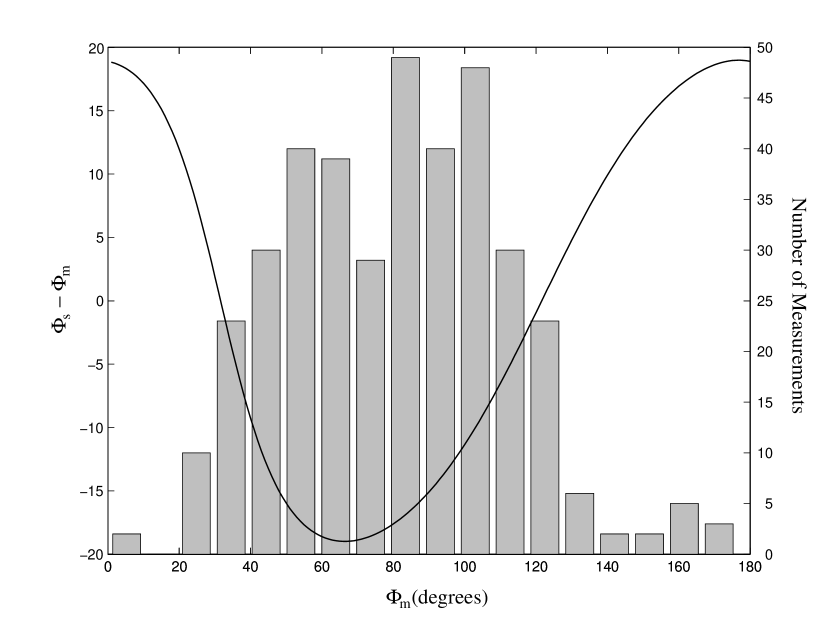
Figure 7: The difference between the intrinsic source polarization angle and the measured polarization angle is plotted as a function of measured polarization angle. This study assumes a toroidal reference beam polarization. Also shown is the distribution of measured polarization angles used in this study.

The difference between the measured and actual polarization angle ($\Phi_{\mathrm{s}}-\Phi_{\mathrm{m}}$) under the above assumptions is plotted versus measured polarization angle ($\Phi_{\mathrm{m}}$) in Figure 7. The maximum error in ($\Phi_{\mathrm{s}}-\Phi_{\mathrm{m}}$) is $\pm$20^∘. Note that the amplitude of this error is independent of the chosen value of $\Phi_{\mathrm{r}}$ since the curve simply shows the error in the measured polarization angle as a function of the difference between the measured polarization angle and the reference beam polarization angle. (In this case, we have set the reference beam polarization angle to an “arbitrary” value.) The potential error induced by reference beam contamination is systematically about twice that of our maximum allowable statistical error. (A signal-to-noise ratio of 3 implies $\sigma_{\phi}\sim 10^{\circ}$.) Though this is potentially large, it is not large enough to cause poloidal fields to be measured as toroidal and vice-versa. Therefore, it is unlikely that the relationship shown in Figures 5 and 6 is caused by reference beam contamination.

We can quantitatively estimate the potential effect of reference beam contamination on the data. This histogram in Figure 7 shows the number of measurements having a polarization angle in each of the 10^∘ bins. As an unfortunate coincidence, the error is not symmetric with respect to our data and thus it is expected that there will be a bias in our field strength estimate. We have applied this correction to the data and the resulting $\phi$ v. $F$ plots have the same basic appearance; however the equilibrium point once the correction is applied is 168$\pm$2 Jy (SHARC beam)^-1. This implies a 30 % increase in our magnetic field strength estimate.

It must be noted that because the large scale field in the Galactic center has been found to be toroidal by Novak et al. (2002), it is possible that a significant amount of dust is present along the line of sight to the central 30 pc that is permeated by this toroidal field and will emit polarized radiation accordingly. In this case, the large scale contribution to the polarized flux can be modeled by a uniform sheet of polarized flux. In this case, chopping can be an advantage in observing magnetic fields in the central 30 pc as it removes the contribution from a uniform field in the foreground and background dust. This model may also explain the lack of polarization measurements by Novak et al. (2002) in the central 30 pc in regions where Hertz sees a poloidal field. Because of the 6′chop, Hertz may be sampling a smaller volume along the line of sight than that of Novak et al. (2002). In the latter case, line-of-sight superposition of the uniform sheet and the polarized emission detected by Hertz may cancel, resulting in unpolarized radiation.

4 Conclusions

As described above, submillimeter and far-infrared polarimetry provides an additional method for estimating the magnetic field strength at the Galactic center, a quantity that has proven to be controversial. Yusef-Zadeh et al. (1997) have argued that the magnetic field strength must exceed $\sim$1 mG in order to maintain the linearity of the NTFs. On the other hand, Sofue et al. (1987) have derived fields of 10-100 $\mu$G for the Arched filaments and the Radio Arc using Faraday rotation measurements. Using equipartition arguments, Tsuboi et al. (1986) have found a field of the same order in the plumes that make up the extension of the Radio Arc on the eastern side of the Galactic Center Lobe. More recently, Zeeman splitting measurements have been done in the central 30 pc both using OH masers and H I emission (Yusef-Zadeh et al., 1996; Plante et al., 1995; Killeen et al., 1992). These studies show a line-of-sight field of a few mG.

Our estimate is in agreement with the notion that there is a pervasive mG field in the Galactic center, thought obtaining a more accurate number will require a larger sample of polarization measurements with corresponding fluxes.

It has been discovered that many of the NTFs in the Galactic center are associated with molecular clouds (Serabyn & Güsten, 1991; Staguhn et al., 1998). This has led to the suggestion that the source of the relativistic electrons in the NTFs is due to magnetic reconnection (Serabyn & Morris, 1994). The magnetic reconnection is believed to be precipitated by the collision of the cloud with a magnetic flux tube either by distorting the fields in the flux tube or by forcing these fields into contact with those in the cloud.

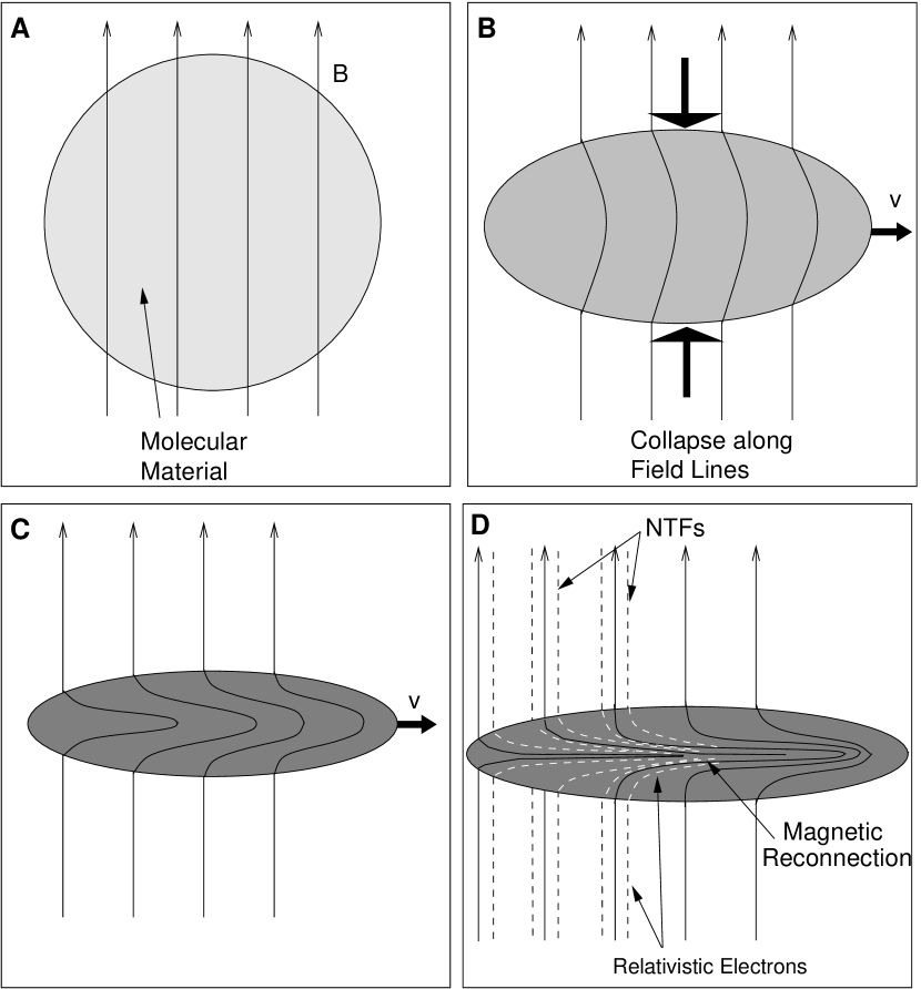
Figure 8: Molecular clouds can produce relativistic electrons necessary for the illumination of NTFs by the following process. In regions of low density, the molecular material is dominated by the magnetic field, and we observe a poloidal field (A). MHD allows for movement of material along the lines of flux. In this way, the material can form clouds and gravity can begin to compete with the magnetic field energy density (B). At this stage, velocities of the molecular material with respect to the poloidal field can distort the field. This process continues (C) as the poloidal fields become sheared into toroidal ones in the vicinity of the cloud. Finally, oppositely-oriented magnetic fields near the cloud centers will be forced into contact by gravity and will reconnect, thereby releasing energy that energizes relativistic electrons. These electrons spiral along the external field and produce synchrotron radiation that we observe as an NTF.

The notion that the poloidal and toroidal fields have the same origin suggests a third option for the magnetic reconnection scenario. Figure 8 illustrates this idea.

In the Galactic center, relatively diffuse molecular gas is supported by magnetic pressure (Fig. 8A); however, this material is free to collapse along the field lines. As the gas collapses, gravitational energy becomes increasingly important. Gravity can accelerate the cloud and the resulting differential motion between the material in the cloud and that of the ambient medium can begin to shear the magnetic field (Fig. 8B). This shear continues until the field is more toroidal than poloidal (Fig. 8C). Note that the field external to the clouds is still quite poloidal because magnetic energy dominates the dynamics of this region. Finally, if the gravitational energy is large enough, and the system is given the time to evolve, the oppositely-oriented fields in the center of the cloud may be squeezed together to enable reconnection. This process releases energy that can produce the relativistic electrons required to “light up” the filaments.

Submillimeter and far-infrared polarimetry in concert with radio and submillimeter photometric observations present a picture of molecular material of various sizes at various evolutionary stages according Figure 8. From the polarimetry data in Figure 1, we can see examples of each of the four panels in Figure 8. The area to the north and east of M-0.02-0.07 is an example of the situation depicted in Figure 8A. Here, the molecular material is not very dense and the magnetic field is perpendicular to the Galactic plane. An example of Figure 8B is the molecular cloud complex containing M0.07-0.08 and M0.11-0.08. Here the field is seen to be shearing around the front edge of M0.07-0.08, making a transition from poloidal to toroidal at the southern edge of the cloud. The 20 km s^-1 cloud (M-0.13-0.08) is thought to be shearing out its magnetic field as it falls toward Sgr A* (Novak et al., 2000). The flare seen at the southern end may indicate that it has not yet reached the point where magnetic reconnection is occurring and hence best matches Figure 8C.

The interaction of the Sickle with the GCRA gives the best example of Figure 8D. Here, the magnetic field in the molecular cloud is observed to be nearly perfectly aligned with the direction of both the long axis of the cloud and the Galactic plane. Filaments, namely those of the GCRA, are observed, and appear to diffuse into G0.18-0.04, the H II region associated with this interaction. The clumpiness of the H II region and the structure of the filaments themselves may stem from the irregularities of the interior of the cloud where reconnection takes place.

It is possible that there are similar occurrences in places such as the Arched Filaments where there is also an observed transition from toroidal to poloidal fields adjacent to an NTF (in this case, the Northern Thread). In order to test this idea with respect to other filaments and clouds in the Galactic center, more complete polarimetric coverage of the central 30 parsecs is required.

Other scenarios for the explanation of the variety of fields in the central 30 pc cannot yet be ruled out. Winds produced by large explosions could be responsible for the poloidal fields seen in this region. However, there are several reasons to favor the association of the poloidal fields with a global field. First of all, the spatial proximity of the poloidal fields in the dust to the NTFs lends evidence to this association. Second, the $\sim$3 mG field strength we derive is consistent with lower limits of the field found in NTFs. Third, to date we have not been able to locate any sources of a wind on large enough scales that couple to the magnetic field geometries observed. Finally, we see transitions from poloidal to toroidal fields that correspond to dynamics of Galactic center molecular clouds, indicating that these two fields have the same origin and that the initial configuration was poloidal.

Table 1: M-0.13-0.08

$\Delta\alpha$	$\Delta\delta$	$P(\%)$	$\sigma_{P}$	$\phi(^{\circ})$	$\sigma_{\phi}$
$-54$	$72$	$3.04$	$1.06$	$108.1$	$8.6$
$-36$	$72$	$2.21$	$0.71$	$99.1$	$9.0$
$-36$	$90$	$2.61$	$0.94$	$100.2$	$9.8$
$-36$	$108$	$4.98$	$1.48$	$102.4$	$7.8$
$18$	$-54$	$1.21$	$0.41$	$107.3$	$9.4$
$36$	$-54$	$1.41$	$0.40$	$91.3$	$8.1$
$54$	$-36$	$1.41$	$0.42$	$70.5$	$8.7$
$72$	$-90$	$1.83$	$0.57$	$97.4$	$8.7$
$72$	$-54$	$2.07$	$0.48$	$82.2$	$6.7$
$90$	$-54$	$2.46$	$0.57$	$87.2$	$6.6$
$108$	$-54$	$2.20$	$0.70$	$58.8$	$9.5$

Table 2: CO+0.02-0.02

$\Delta\alpha$	$\Delta\delta$	$P(\%)$	$\sigma_{P}$	$\phi(^{\circ})$	$\sigma_{\phi}$
$-54$	$-18$	$2.76$	$0.85$	$107.6$	$8.8$
$-54$	$18$	$2.75$	$0.74$	$88.5$	$7.7$
$-36$	$-54$	$3.66$	$1.14$	$107.7$	$9.0$
$-36$	$-36$	$3.17$	$0.60$	$103.8$	$5.4$
$-36$	$-18$	$2.66$	$0.59$	$100.2$	$6.2$
$-36$	$0$	$3.16$	$0.63$	$91.3$	$5.7$
$-36$	$18$	$1.82$	$0.59$	$85.4$	$9.4$
$-36$	$36$	$3.08$	$0.73$	$80.3$	$6.8$
$-18$	$-54$	$3.20$	$0.89$	$112.8$	$8.2$
$-18$	$-36$	$1.46$	$0.39$	$98.0$	$7.7$
$-18$	$-18$	$1.74$	$0.42$	$78.5$	$6.9$
$-18$	$0$	$2.72$	$0.55$	$83.2$	$5.8$
$-18$	$18$	$2.33$	$0.56$	$66.4$	$6.8$
$-18$	$36$	$2.02$	$0.57$	$68.9$	$8.2$
$-18$	$54$	$2.20$	$0.69$	$63.2$	$9.6$
$0$	$-36$	$1.74$	$0.36$	$81.8$	$6.0$
$0$	$-18$	$2.09$	$0.32$	$95.2$	$4.3$
$0$	$0$	$1.13$	$0.32$	$75.1$	$8.2$
$0$	$18$	$1.88$	$0.43$	$79.6$	$6.5$
$0$	$36$	$2.75$	$0.45$	$60.7$	$4.7$
$0$	$54$	$2.47$	$0.80$	$79.0$	$9.6$
$18$	$-36$	$1.33$	$0.34$	$79.1$	$7.2$
$18$	$-18$	$2.13$	$0.30$	$91.3$	$4.1$
$18$	$0$	$1.18$	$0.27$	$73.3$	$6.6$
$18$	$18$	$2.27$	$0.39$	$63.7$	$4.9$
$18$	$36$	$3.08$	$0.60$	$76.5$	$5.7$
$36$	$-36$	$1.71$	$0.59$	$75.4$	$9.9$
$36$	$-18$	$1.69$	$0.38$	$68.6$	$6.5$
$36$	$0$	$1.98$	$0.30$	$67.6$	$4.3$
$36$	$18$	$2.43$	$0.52$	$63.5$	$6.3$
$36$	$36$	$3.53$	$0.85$	$67.7$	$7.0$
$54$	$-18$	$2.23$	$0.75$	$58.7$	$9.8$
$54$	$0$	$3.22$	$0.70$	$63.3$	$6.9$

Table 3: NW of M-0.02-0.07

$\Delta\alpha$	$\Delta\delta$	$P(\%)$	$\sigma_{P}$	$\phi(^{\circ})$	$\sigma_{\phi}$
$-54$	$0$	$2.13$	$0.51$	$102.8$	$7.1$
$-54$	$36$	$1.68$	$0.47$	$80.7$	$8.0$
$-36$	$18$	$0.97$	$0.32$	$83.0$	$9.4$
$-36$	$36$	$1.45$	$0.40$	$79.0$	$7.8$
$-18$	$-36$	$2.05$	$0.41$	$92.9$	$5.8$
$-18$	$0$	$1.46$	$0.46$	$78.9$	$8.9$
$-18$	$36$	$2.01$	$0.46$	$61.9$	$6.4$
$0$	$36$	$1.33$	$0.46$	$73.3$	$9.7$
$18$	$-36$	$1.07$	$0.30$	$60.8$	$7.8$
$18$	$0$	$1.36$	$0.34$	$56.4$	$7.1$
$18$	$18$	$1.63$	$0.37$	$55.5$	$6.4$
$18$	$36$	$1.49$	$0.48$	$60.6$	$9.0$
$18$	$54$	$2.60$	$0.73$	$64.3$	$7.8$
$36$	$-36$	$0.98$	$0.34$	$66.7$	$9.7$
$36$	$-18$	$1.50$	$0.31$	$50.5$	$5.9$
$36$	$0$	$1.12$	$0.33$	$45.5$	$8.4$
$36$	$18$	$2.31$	$0.36$	$58.0$	$4.3$
$36$	$36$	$2.22$	$0.47$	$58.9$	$6.1$
$54$	$-36$	$2.56$	$0.80$	$52.2$	$9.0$

Table 4: NE of M-0.02-0.07

$\Delta\alpha$	$\Delta\delta$	$P(\%)$	$\sigma_{P}$	$\phi(^{\circ})$	$\sigma_{\phi}$
$-54$	$-18$	$0.84$	$0.26$	$68.8$	$9.1$
$-54$	$0$	$0.78$	$0.24$	$62.0$	$8.8$
$-54$	$18$	$1.33$	$0.23$	$55.8$	$5.0$
$-54$	$36$	$1.27$	$0.33$	$43.8$	$7.5$
$-36$	$-18$	$0.88$	$0.23$	$53.1$	$7.5$
$-36$	$18$	$1.17$	$0.21$	$37.2$	$5.0$
$-36$	$36$	$0.81$	$0.22$	$38.1$	$7.4$
$-36$	$54$	$1.13$	$0.35$	$48.7$	$9.1$
$-18$	$-36$	$1.52$	$0.22$	$57.9$	$4.4$
$-18$	$-18$	$1.46$	$0.23$	$43.4$	$4.5$
$-18$	$0$	$1.28$	$0.25$	$42.5$	$5.6$
$-18$	$18$	$1.46$	$0.37$	$42.2$	$7.2$
$-18$	$36$	$1.70$	$0.28$	$29.2$	$4.5$
$-18$	$54$	$2.35$	$0.36$	$42.7$	$4.4$
$0$	$-36$	$1.44$	$0.25$	$54.6$	$5.2$
$0$	$-18$	$1.58$	$0.26$	$41.0$	$4.6$
$0$	$0$	$1.58$	$0.26$	$39.5$	$4.7$
$0$	$18$	$1.92$	$0.42$	$29.4$	$5.8$
$0$	$36$	$1.99$	$0.40$	$44.0$	$5.7$
$0$	$54$	$2.16$	$0.45$	$47.3$	$6.0$
$18$	$-54$	$2.30$	$0.55$	$65.5$	$7.2$
$18$	$-36$	$1.08$	$0.30$	$41.1$	$7.9$
$18$	$-18$	$1.13$	$0.33$	$44.5$	$8.4$
$18$	$0$	$1.90$	$0.41$	$25.7$	$5.8$
$18$	$18$	$1.75$	$0.46$	$38.0$	$7.4$
$18$	$36$	$2.94$	$0.65$	$34.3$	$6.1$
$18$	$54$	$3.25$	$0.72$	$49.4$	$6.5$
$36$	$-36$	$1.81$	$0.51$	$45.0$	$8.1$
$36$	$-18$	$1.20$	$0.44$	$20.7$	$9.9$
$36$	$18$	$3.30$	$0.60$	$29.0$	$5.0$
$54$	$0$	$4.63$	$1.09$	$37.7$	$7.0$
$54$	$18$	$6.69$	$1.41$	$32.9$	$6.0$

Table 5: E of M-0.02-0.07

$\Delta\alpha$	$\Delta\delta$	$P(\%)$	$\sigma_{P}$	$\phi(^{\circ})$	$\sigma_{\phi}$
$-54$	$-36$	$1.49$	$0.31$	$58.5$	$6.5$
$-54$	$-18$	$1.03$	$0.18$	$49.7$	$5.1$
$-54$	$0$	$1.26$	$0.16$	$49.3$	$3.5$
$-54$	$18$	$1.18$	$0.16$	$53.7$	$3.9$
$-54$	$36$	$1.44$	$0.26$	$53.0$	$5.0$
$-36$	$-54$	$1.38$	$0.38$	$54.7$	$8.1$
$-36$	$-36$	$1.30$	$0.22$	$43.5$	$4.8$
$-36$	$-18$	$0.67$	$0.18$	$47.3$	$7.6$
$-36$	$0$	$0.71$	$0.17$	$43.8$	$6.6$
$-36$	$18$	$0.80$	$0.16$	$39.1$	$5.8$
$-36$	$36$	$1.60$	$0.21$	$35.2$	$3.6$
$-36$	$54$	$1.34$	$0.38$	$41.3$	$8.2$
$-18$	$-54$	$2.38$	$0.56$	$34.4$	$6.5$
$-18$	$-18$	$0.59$	$0.19$	$37.5$	$9.2$
$-18$	$18$	$1.18$	$0.24$	$24.2$	$5.9$
$-18$	$36$	$2.15$	$0.23$	$36.1$	$3.0$
$-18$	$54$	$1.44$	$0.39$	$25.2$	$8.1$
$0$	$-54$	$2.25$	$0.64$	$51.1$	$8.2$
$0$	$-36$	$1.82$	$0.30$	$37.3$	$4.7$
$0$	$-18$	$1.52$	$0.21$	$31.0$	$4.0$
$0$	$0$	$1.15$	$0.21$	$39.6$	$5.1$
$0$	$18$	$1.94$	$0.26$	$37.9$	$3.8$
$0$	$36$	$2.53$	$0.32$	$28.0$	$3.6$
$0$	$54$	$2.27$	$0.56$	$37.6$	$7.3$
$18$	$-18$	$1.27$	$0.25$	$27.6$	$5.5$
$18$	$0$	$0.94$	$0.27$	$34.2$	$8.3$
$18$	$18$	$2.13$	$0.34$	$34.1$	$4.7$
$18$	$36$	$3.25$	$0.52$	$38.4$	$4.6$
$18$	$54$	$3.55$	$0.79$	$31.2$	$6.7$
$36$	$-18$	$1.61$	$0.35$	$29.8$	$6.4$
$36$	$0$	$2.25$	$0.38$	$39.7$	$4.9$
$36$	$18$	$2.48$	$0.45$	$39.1$	$5.2$
$36$	$36$	$4.00$	$1.19$	$41.0$	$8.6$

Table 6: M+0.07-0.08

$\Delta\alpha$	$\Delta\delta$	$P(\%)$	$\sigma_{P}$	$\phi(^{\circ})$	$\sigma_{\phi}$
$-54$	$-18$	$2.64$	$0.88$	$49.3$	$9.5$
$-36$	$-18$	$1.76$	$0.47$	$60.7$	$7.8$
$-36$	$0$	$2.54$	$0.83$	$54.8$	$9.0$
$-36$	$36$	$5.82$	$1.97$	$46.2$	$9.6$
$-18$	$-54$	$2.04$	$0.60$	$37.4$	$8.6$
$-18$	$-36$	$1.44$	$0.27$	$45.0$	$5.4$
$-18$	$-18$	$1.18$	$0.28$	$48.1$	$6.8$
$-18$	$0$	$1.65$	$0.52$	$47.2$	$9.0$
$-18$	$18$	$2.16$	$0.76$	$57.6$	$9.2$
$0$	$-54$	$1.17$	$0.40$	$176.2$	$9.9$
$0$	$-36$	$1.13$	$0.23$	$4.4$	$5.8$
$0$	$0$	$0.62$	$0.22$	$55.2$	$9.9$
$18$	$-54$	$1.74$	$0.46$	$160.0$	$7.3$
$18$	$-18$	$0.88$	$0.23$	$158.1$	$7.5$
$18$	$54$	$2.39$	$0.80$	$131.4$	$9.5$
$36$	$-36$	$1.79$	$0.49$	$158.1$	$7.3$
$36$	$-18$	$2.13$	$0.30$	$138.7$	$4.0$

Table 7: M+0.11-0.08

$\Delta\alpha$	$\Delta\delta$	$P(\%)$	$\sigma_{P}$	$\phi(^{\circ})$	$\sigma_{\phi}$
$-54$	$18$	$1.99$	$0.46$	$74.9$	$6.9$
$-54$	$36$	$1.62$	$0.55$	$73.2$	$9.9$
$-36$	$-36$	$1.09$	$0.35$	$113.1$	$9.2$
$-36$	$54$	$2.25$	$0.51$	$35.6$	$6.6$
$-18$	$36$	$1.14$	$0.29$	$61.7$	$7.6$
$18$	$-54$	$2.01$	$0.60$	$0.4$	$8.5$
$18$	$-36$	$0.84$	$0.22$	$174.3$	$7.6$
$18$	$-18$	$1.02$	$0.19$	$161.1$	$5.4$
$18$	$0$	$0.73$	$0.19$	$125.8$	$7.3$
$36$	$-36$	$1.95$	$0.43$	$168.1$	$6.5$
$36$	$-18$	$0.75$	$0.24$	$166.3$	$9.3$
$36$	$18$	$0.93$	$0.28$	$151.3$	$8.9$
$54$	$0$	$1.42$	$0.46$	$140.1$	$9.4$

Figure 5: The absolute value of the deviation of each measurement from a poloidal field is plotted against 350 $\mu$m flux in a 15^′′ SHARC beam. Here the angles are used from all of the GC polarization measurements. The assumption is that the polarization angle will not change significantly from 60 $\mu$m to 350 $\mu$m.

References

- Davidson (1996) Davidson, J. A. 1996, in ASP Conference Series, Vol. 97, Polarimetry of the Interstellar Medium, ed. W. G. Roberge & D. C. B. Whittet, San Francisco, 504–521
- Dotson (1986) Dotson, J. L. 1986, ApJ, 470, 566
- Dotson et al. (2000) Dotson, J. D., Davidson, J., Dowell, C. D., Schleuning, D. A., & Hildebrand, R. H. 2000, ApJS, 128, 335
- Dowell et al. (1998) Dowell, C. D., Hildebrand, R. H., Schleuning, D. A., Vaillancourt, J. E., Dotson, J. L., Novak, G., Renbarger, T., & Houde, M. 1998, ApJ, 504, 588
- Dowell et al. (1999) Dowell, C. D., Lis, D. C., Serabyn, E., Gardner, M., Kovacs, A., & Yamashita, S. 1999, in ASP Conference Series 186: The Central Parsecs of the Galaxy, ed. H. Falcke, A. Cotera, W. Duschl, F. Melia, & M. Rieke, 453–465
- Ho et al. (1991) Ho, P. T. P., Ho, L. C., Szczepanski, J. C., Jackson, J. M., & Armstrong, J. T. 1991, Nature, 350, 309
- Killeen et al. (1992) Killeen, N. E. B., Lo, K. Y., & Crutcher, R. 1992, ApJ, 385, 585
- LaRosa et al. (2000) LaRosa, T. N., Kassim, N. E., Lazio, T. J. W., & Hyman, S. D. 2000, ApJ, 119, 207
- Matthews et al. (2002) Matthews, B. C., Fiege, J. D., & Moriarty-Schieven, G. 2002, ApJ, 569, 304
- Matthews et al. (2001) Matthews, B. C., Wilson, C. D., & Fiege, J. D. 2001, ApJ, 562, 400
- Morris & Serabyn (1996) Morris, M., & Serabyn, E. 1996, ARAA, 34, 645
- Novak et al. (2002) Novak, G., Chuss, D., Renbarger, T., Griffin, G. S., Newcomb, M. G., Peterson, J. B., Loewenstein, R. F., Pernic, D., & Dotson, J. L. 2002, in press
- Novak et al. (1997) Novak, G., Dotson, J. L., Dowell, C. D., Goldsmith, P. F., Hildebrand, R. H., Platt, S. R., & Schleuning, D. A. 1997, ApJ, 487, 320
- Novak et al. (2000) Novak, G., Dotson, J. L., Dowell, C. D., Hildebrand, R. H., Renbarger, T., & Schleuning, D. A. 2000, ApJ, 529, 241
- Okumura et al. (1991) Okumura, S. K., Ishiguro, M., Kasuga, T., Morita, K., Kawabe, R., Fomalont, E. B., Hasegawa, T., & Kobayashi, H. 1991, ApJ, 378, 127
- Pierce-Price et al. (2000) Pierce-Price, D., Richer, J. S., Greaves, J. S., Holland, W. S., Jenness, T., Lasenby, A. N., White, G. J., Matthews, H. E., Ward-Thompson, D., Dent, W. R. F., Zykla, R., Mezger, P., Hasegawa, T., Oka, T., Omont, A., & Gilmore, G. 2000, ApJ, 545, L121
- Plante et al. (1995) Plante, R. L., Lo, K. Y., & Crutcher, R. M. 1995, ApJ, 445, L113
- Price et al. (2001) Price, S. D., Egan, M. P., Carey, S. J., Mizuno, D. R., & Kuchar, T. A. 2001, ApJ, 121, 2819
- Schleuning (1988) Schleuning, D. A. 1988, ApJ, 493, 811
- Schleuning et al. (1997) Schleuning, D. A., Dowell, C. D., Hildebrand, R. H., & Platt, S. R. 1997, PASP, 109, 307
- Serabyn & Güsten (1991) Serabyn, E., & Güsten, R. 1991, A & A, 242, 376
- Serabyn & Morris (1994) Serabyn, E., & Morris, M. 1994, ApJ, 424, L91
- Serkowski (1974) Serkowski, K. 1974, in Methods of Experimental Physics Volume 12 - Part A: Atrophysics - Optical and Infrared, ed. N. Carleton (New York: Academic Press), 361–416
- Sofue et al. (1987) Sofue, Y., Reich, W., Inoue, M., & Seiradakis, J. H. 1987, PASJ, 39, 95
- Staguhn et al. (1998) Staguhn, J., Stutski, J., Uchida, K. I., & Yusef-Zadeh, F. 1998, ApJ, 336, 290
- Tsuboi et al. (1986) Tsuboi, M., Handa, T., Tabara, H., Kato, T., Sofue, Y., & Kaifu, N. 1986, AJ, 92, 818
- Tsuboi et al. (1999) Tsuboi, M., Handa, T., & Ukita, N. 1999, ApJ, 120, 1
- Tsuboi et al. (1997) Tsuboi, M., Ukita, N., & Handa, T. 1997, ApJ, 481, 263
- Uchida et al. (1985) Uchida, Y., Shibata, K., & Sofue, Y. 1985, Nature, 317, 699
- Yusef-Zadeh et al. (1984) Yusef-Zadeh, F., Morris, M., & Chance, D. 1984, Nature, 310, 557
- Yusef-Zadeh et al. (1996) Yusef-Zadeh, F., Roberts, D. A., Goss, W. M., Frail, D. A., & Green, A. J. 1996, ApJ, 466, L25
- Yusef-Zadeh et al. (1997) Yusef-Zadeh, F., Wardle, M., & Parastaran, P. 1997, ApJ, 475, L119
- Yusef-Zadeh & Morris (1987) Yusef-Zadeh, F., & Morris, M. 1987, ApJ, 320, 545
- Zylka et al. (1990) Zylka, R., Mezger, P. G., & Wink, J. E. 1990, A & A, 234, 133