A Hybrid Cosmological Hydrodynamic/N-body Code Based on the Weighted Essentially Non-Oscillatory Scheme

Abstract

We describe a newly developed cosmological hydrodynamics code based on the weighted essentially non-oscillatory (WENO) schemes for hyperbolic conservation laws. High order finite difference WENO schemes are designed for problems with piecewise smooth solutions containing discontinuities, and have been successful in applications for problems involving both shocks and complicated smooth solution structures. We couple hydrodynamics based on the WENO scheme with standard Poisson solver - particle-mesh (PM) algorithm for evolving the self-gravitating system. A third order total variation diminishing (TVD) Runge-Kutta scheme has been used for time-integration of the system. We brief the implementation of numerical technique. The cosmological applications in simulating intergalactic medium and Ly$\alpha$ forest in the CDM scenario are also presented.

1 Introduction

Due to the highly non-linearity of gravitational clustering in the universe, one significant feature emerging in cosmological hydrodynamic flow is extremely supersonic motion around the density peaks developed by gravitational instability, which leads to strong shock discontinuities within complex smooth structures. It poses more challenge than the typical hydrodynamic simulation without self-gravity. To address this issue, two algorithms have been implemented for high resolution shock capturing in cosmology: total-variation diminishing (TVD) scheme^[1] and piecewise parabolic method (PPM)^[2].

An alternative hydrodynamic solver to discretize the convection terms in the Euler equations is the fifth order finite difference WENO (weighted essentially non-oscillatory) method^[3], with a low storage nonlinearly stable third order Runge-Kutta time discretization^[4]. The WENO schemes, first constructed in third order finite volume version by Liu et al.^[5], are based on the essentially non-oscillatory scheme (ENO) developed by Harten et al.^[6] in the form of finite volume scheme for hyperbolic conservative laws. The ENO scheme generalizes the total variation diminishing (TVD) scheme of Harten. The TVD schemes typically degenerate to first-order accuracy at locations with smooth extrema while the ENO and WENO schemes maintain high order accuracy there even in multi-dimensions. The WENO method is very robust and stable for solutions containing strong shocks and complex solution structures^[3],[5]. It uses the idea of adaptive stencils in the reconstruction procedure based on the local smoothness of the numerical solution to automatically achieve high order accuracy and non-oscillatory property near discontinuities. This is achieved by using a convex combination of a few candidate stencils, each being assigned a nonlinear weight which depends on the local smoothness of the numerical solution based on that stencil. WENO schemes can simultaneously provide a high order resolution for the smooth part of the solution, and a sharp, monotone shock or contact discontinuity transition.

In the context of cosmological applications, we have developed a hybrid N-body/hydrodynamical code that incorporates a Lagrangian particle-mesh algorithm to evolve the collision-less matter with the fifth order WENO scheme to solve the equation of gas dynamics. This paper describes this code briefly.

2 Numerical Techniques

2.1 The Basic Equations

The hydrodynamic equations for baryons in the expanding universe, without any viscous and thermal conductivity terms, can be written as,

$$\dot{U}+\partial_{i}{\bf F}^{i}[U]=f(t,U)$$ (1)

where the abbreviation $\partial_{i}\equiv\partial/\partial x^{i}$ has been used, $x^{i}$ denote the proper coordinates. $U$ is a five-component column vector, $U=(\rho,\rho v_{1},\rho v_{2},\rho v_{3},E)$, $\rho$ is the comoving density, ${\bf v}=\{v_{i}\}$ is the proper peculiar velocity, E is the total energy per unit comoving volume including both kinetic and internal energy, P is comoving pressure, related to the total energy E by $E=P/(\gamma-1)+\frac{1}{2}\rho{\bf v}^{2}$ where we assume an ideal gas equation of state, $P=(\gamma-1)e$, where $e$ is the internal energy density and $\gamma$ is the ratio of the specific heats of the baryon. The left hand side of Eq.(1) is written in the conservative form for mass, momentum and energy, the ”force” source term on right hand side includes the contributions from the expansion of the universe, the gravitation. $\Lambda_{net}$ in the energy equation represents the net energy loss due to the radiative heating-cooling of the baryonic gas.

$$f(t,U)=(0,-\frac{\dot{a}}{a}\rho{\bf v}+\rho{\bf g},-2\frac{\dot{a}}{a}E+\rho{\bf v}\cdot{\bf g}-\Lambda_{cool})$$ (2)

where ${\bf g}$ is the peculiar acceleration in the gravitational field produced by both the dark matter and the baryonic matter, which is obtained by solving the Poisson equation using standard particle-mesh technique.

2.2 Hydrodynamic Solver: Finite Difference WENO Schemes

The fifth order WENO finite difference spatial discretization to a conservation law such as

$$u_{t}+f(u)_{x}+g(u)_{y}=0$$ (3)

approximates the derivatives, for example $f(u)_{x}$, by a conservative difference

$$f(u)_{x}|_{x=x_{j}}\approx\frac{1}{\Delta x}\left(\hat{f}_{j+1/2}-\hat{f}_{j-1/2}\right)$$

where $\hat{f}_{j+1/2}$ is the numerical flux. $g(u)_{y}$ is approximated in the same way. Hence finite difference methods have the same format for one and several space dimensions, which is a major advantage. For the simplest case of a scalar equation (3) and if $f^{\prime}(u)\geq 0$, the fifth order finite difference WENO scheme has the flux given by

$$\hat{f}_{j+1/2}=w_{1}\hat{f}_{j+1/2}^{(1)}+w_{2}\hat{f}_{j+1/2}^{(2)}+w_{3}\hat{f}_{j+1/2}^{(3)}$$

where $\hat{f}_{j+1/2}^{(i)}$ are three third order accurate fluxes on three different stencils given by

$$\hat{f}_{j+1/2}^{(1)} = \frac{1}{3}f(u_{j-2})-\frac{7}{6}f(u_{j-1})+\frac{11}{6}f(u_{j}),$$

$$\hat{f}_{j+1/2}^{(2)} = -\frac{1}{6}f(u_{j-1})+\frac{5}{6}f(u_{j})+\frac{1}{3}f(u_{j+1}),$$

$$\hat{f}_{j+1/2}^{(3)} = \frac{1}{3}f(u_{j})+\frac{5}{6}f(u_{j+1})-\frac{1}{6}f(u_{j+2}).$$

Notice that the combined stencil for the flux $\hat{f}_{j+1/2}$ is biased to the left, which is upwinding for the positive wind direction due to the assumption $f^{\prime}(u)\geq 0$. The key ingredient for the success of WENO scheme relies on the design of the nonlinear weights $w_{i}$, which are given by

$$w_{i}=\frac{\tilde{w}_{i}}{\sum_{k=1}^{3}\tilde{w}_{k}},\qquad\tilde{w}_{k}=\frac{\gamma_{k}}{(\varepsilon+\beta_{k})^{2}},$$

where the linear weights $\gamma_{k}$ are chosen to yield fifth order accuracy when combining three third order accurate fluxes, and are given by

$$\gamma_{1}=\frac{1}{10},\qquad\gamma_{2}=\frac{3}{5},\qquad\gamma_{3}=\frac{3}{10};$$

the smoothness indicators $\beta_{k}$ are given by

$$\beta_{1} = \frac{13}{12}\left(f(u_{j-2})-2f(u_{j-1})+f(u_{j})\right)^{2}+\frac{1}{4}\left(f(u_{j-2})-4f(u_{j-1})+3f(u_{j})\right)^{2}$$

$$\beta_{2} = \frac{13}{12}\left(f(u_{j-1})-2f(u_{j})+f(u_{j+1})\right)^{2}+\frac{1}{4}\left(f(u_{j-1})-f(u_{j+1})\right)^{2}$$

$$\beta_{3} = \frac{13}{12}\left(f(u_{j})-2f(u_{j+1})+f(u_{j+2})\right)^{2}+\frac{1}{4}\left(3f(u_{j})-4f(u_{j+1})+f(u_{j+2})\right)^{2},$$

and they measure how smooth the approximation based on a specific stencil is in the target cell. Finally, $\varepsilon$ is a parameter to avoid the denominator to become zero and is usually taken as $\varepsilon=10^{-6}$ in the computation.

This finishes the description of the fifth order finite difference WENO scheme^[3] in the simplest case. As we can see, the algorithm is actually quite simple and the user does not need to tune any parameters in the scheme.

The WENO finite difference scheme is characterized by the following properties. (1) The scheme is proven to be uniformly fifth order accurate including at smooth extrema, and this is verified numerically. (2) Near discontinuities the scheme produces sharp and non-oscillatory discontinuity transition. (3) The approximation is self-similar. That is, when fully discretized with the Runge-Kutta methods discussed in next section §2.3, the scheme is invariant when the spatial and time variables are scaled by the same factor. This is a major advantage for approximating conservation laws which are invariant under such scaling. For the details of how the scheme can be generalized in a more complex situation, eventually to 3D systems such as Euler equations, we refer to the reference [7].

2.3 Time Discretizations

To further discretize in time, we use a class of high order nonlinearly stable Runge-Kutta time discretizations. A distinctive feature of this class of time discretizations is that they are convex combinations of first order forward Euler steps, hence they maintain strong stability properties in any semi-norm (total variation norm, maximum norm, entropy condition, etc.) of the forward Euler step, with a time step restriction proportional to that for the forward Euler step to be stable, this proportion coefficient being termed CFL coefficient of the high order Runge-Kutta method^[8]. The most popular scheme in this class is the following third order Runge-Kutta method for solving $u_{t}=L(u,t)$, where $L(u,t)$ is a spatial discretization operator:

$$u^{(1)} = u^{n}+\Delta tL(u^{n},t^{n})$$

$$u^{(2)} = \frac{3}{4}u^{n}+\frac{1}{4}u^{(1)}+\frac{1}{4}\Delta tL(u^{(1)},t^{n}+\Delta t)$$ (4)

$$u^{n+1} = \frac{1}{3}u^{n}+\frac{2}{3}u^{(2)}+\frac{2}{3}\Delta tL(u^{(2)},t^{n}+\frac{1}{2}\Delta t),$$

which is nonlinearly stable with a CFL coefficient 1.0. However, for our purpose of 3D calculations, storage is a paramount consideration. We thus use the third order low storage nonlinearly stable Runge-Kutta method which was proven to be nonlinearly stable in [4], with a CFL coefficient 0.32.

The timestep is chosen by the minimum value among three time scales. The first is from the Courant condition given by

$$\Delta t\leq\frac{CFL\times a(t)\Delta x}{\hbox{max}(|u_{x}|+c_{s},|u_{y}|+c_{s},|u_{z}|+c_{s})}$$ (5)

where $\Delta x$ is the cell size, $c_{s}$ is the local sound speed, $u_{x}$, $u_{y}$ and $u_{z}$ are the local fluid velocities and $CFL$ is the Courant number, typically, we take $CFL=0.3$. The second constraint is imposed by cosmic expansion which requires that $\Delta a/a<0.02$ within single time step. The last constraint comes from the requirement that a particle move no more than a fixed fraction of cell size in one time step.

3 Cosmological Application: IGM and Ly$\alpha$ Forest at High Redshift

We run our hybrid N-body/hydrodynamic code to compute the cosmic evolution of coupled system of both dark matter and baryonic matter in a flat low density CDM model ($\Lambda$CDM), which is specified by the cosmological parameters $(\Omega_{m},\Omega_{\Lambda},h,\sigma_{8},\Omega_{b})=(0.3,0.7,0.65,0.9,0.035)$. The simulations were performed in a periodic, cubical box of size 12h^-1Mpc with a 128³ grid and an equal number of dark matter particles. Atomic processes including ionization, radiative cooling and heating are modeled as in Cen^[9] in a primeval plasma of hydrogen and helium of composition ($X=0.76$, $Y=0.24$). The uniform UV-background of ionizing photons is assumed to have a power-law spectrum of the form $J(\nu)=J_{21}\times 10^{-21}(\nu/\nu_{HI})^{-\alpha}$ergs^-1cm^-2sr^-1Hz^-1 parameterized by photoionizing flux $J_{21}$ at the Lyman limit frequency $\nu_{HI}$, and is suddenly switched on at $z\sim 6$ to heat the gas and reionize the universe.

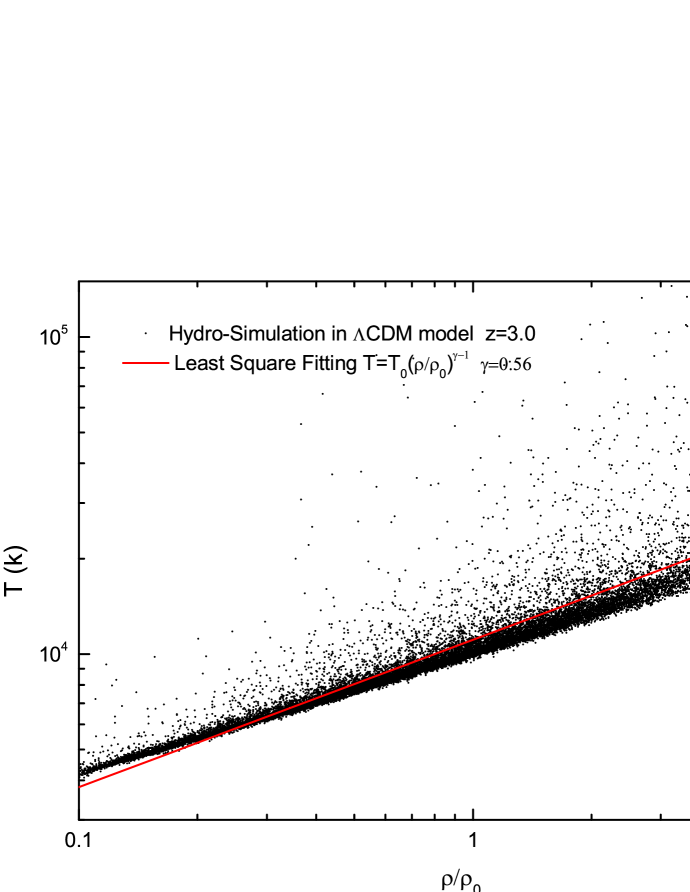
Figure 1: Scatter plot of IGM temperature vs. density relation randomly drawn from a $\Lambda$CDM simulation at redshift $z=3.0$. The line is the least-square-fitting of power-law using each set of points displayed in the figure.

The evolution of the IGM temperature relies on the reionization history of hydrogen and helium, and plays important role in our understanding the Ly$\alpha$ absorption spectrum. It is expected that a power-law relation between IGM temperature and density $T=T_{0}(\rho/<\rho>)^{\gamma-1}$ could be established due to the ionizing photon heating the gas^[10]. We test T versus $\rho$ relation using the simulation samples. Fig.(1) shows the scatter plot of temperature-density relation drawn from the simulation at the output of redshift z=3. Apparently, the T-$\rho$ relation approximates roughly a power law with a best-fitting value of $\gamma=0.56$. The dispersions in temperature at a fixed density mainly arise from the shock-heating.

Mock Ly$\alpha$ spectra are produced along random lines of sight in the simulation box, and meanwhile, the corresponding one-dimension distributions of IGM density and peculiar velocity are also extracted from the sample. The results are demonstrated in Fig.(2). To compare with the observation, e.g. the Keck spectrum of QSO q0014+8118, we Gaussian smooth the spectra to match with the spectral resolutions of observation and normalize the spectra by the observed mean flux decrement. For q0014+8118, we have $D=1-<e^{-\tau}>\approx 0.31$. It could be shown that there are good agreements of flux power spectrum and some higher-order statistical behaviors^[11] (e.g. intermittency) between the observation and simulations^[12].

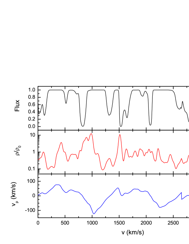
Figure 2: An example of simulated Ly$\alpha$ absorption spectrum and corresponding IGM physical properties along randomly selected line of sight. Upper panel: transmitted flux; middle panel: density distribution of the neutral hydrogen; lower panel: peculiar velocity distribution.

References

- [1] A. Harten, J. Comput. Phys., 49, 357 (1983)
- [2] P. Collela & P.R. Woodward, J. Comput. Phys., 54, 174 (1984)
- [3] G. Jiang & C.-W. Shu, J. Comput. Phys. 126, 202 (1996)
- [4] S. Gottlieb & C.-W. Shu, Math. Comp., 67, 73 (1998)
- [5] X.-D. Liu, S. Osher & T. Chan, J. Comput. Phys., 115, 200 (1994)
- [6] A. Harten, B. Engquist, S. Osher & S. Chakravarthy, J. Comput. Phys. 71, 231 (1987)
- [7] C.-W. Shu, in Advanced Numerical Approximation of Nonlinear Hyperbolic Equations, B. Cockburn, C. Johnson, C.-W. Shu and E. Tadmor (Editor: A. Quarteroni), Lecture Notes in Mathematics,Springer,1697,325 (1998)
- [8] S. Gottlieb, C.-W. Shu & E. Tadmor, SIAM Review, 43, 89 (2001)
- [9] R.Y., Cen, ApJS, 78, 341 (1992)
- [10] L. Hui & Gnedin, N.Y., MNRAS, 292,27 (1997)
- [11] J. Pando, L.L. Feng, P. Jamkhedkar, W. Zheng, D. Kirkman, D. Tytler & L.Z. Fang, ApJ, 574, 575 (2002)
- [12] L.L. Feng, J. Pando & L.Z. Fang, ApJ, accepted, (2002)