Point Source Detection using the Spherical Mexican Hat Wavelet on simulated all-sky Planck maps

Abstract

We present an estimation of the point source (PS) catalogue that could be extracted from the forthcoming ESA Planck mission data. We have applied the Spherical Mexican Hat Wavelet (SMHW) to simulated all-sky maps that include CMB, Galactic emission (thermal dust, free-free and synchrotron), thermal Sunyaev-Zel’dovich effect and PS emission, as well as instrumental white noise . This work is an extension of the one presented in Vielva et al. (2001a). We have developed an algorithm focused on a fast local optimal scale determination, that is crucial to achieve a PS catalogue with a large number of detections and a low flux limit. An important effort has been also done to reduce the CPU time processor for spherical harmonic transformation, in order to perform the PS detection in a reasonable time. The presented algorithm is able to provide a PS catalogue above fluxes: 0.48 Jy (857 GHz), 0.49 Jy (545 GHz), 0.18 Jy (353 GHz), 0.12 Jy (217 GHz), 0.13 Jy (143 GHz), 0.16 Jy (100 GHz HFI), 0.19 Jy (100 GHz LFI), 0.24 Jy (70 GHz), 0.25 Jy (44 GHz) and 0.23 Jy (30 GHz). We detect around 27700 PS at the highest frequency Planck channel and 2900 at the 30 GHz one. The completeness level are: 70% (857 GHz), 75% (545 GHz), 70% (353 GHz), 80% (217 GHz), 90% (143 GHz), 85% (100 GHz HFI), 80% (100 GHz LFI), 80% (70 GHz), 85% (44 GHz) and 80% (30 GHz). In addition, we can find several PS at different channels, allowing the study of the spectral behaviour and the physical processes acting on them. We also present the basic procedure to apply the method in maps convolved with asymmetric beams. The algorithm takes $\sim$ 72 hours for the most CPU time demanding channel (857 GHz) in a Compaq HPC320 (Alpha EV68 1 GHz processor) and requires 4 GB of RAM memory; the CPU time goes as $O(N_{R_{o}}{N_{\rm pix}}^{3/2}log(N_{\rm pix}))$, where $N_{\rm pix}$ is the number of pixels in the map and $N_{R_{o}}$ is the number of optimal scales needed.

1 Introduction

The study of the Cosmic Microwave Background (CMB) anisotropies is one of the most powerful tools to understand the Universe. The CMB power spectrum analysis provides us information about how the Universe was as early as 300000 years after the Big Bang. Acoustic peaks were predicted to be present in the CMB power spectrum for several cosmological models (see Hu et al. 1997 for a review). Recent experiments like BOOMERanG (Netterfield et al. 2002, Rulh et al. 2002), MAXIMA (Hanany et al. 2000), DASI (Halverson et al. 2002), VSA (Rubiño-Martín et al. 2002), CBI (Mason et al. 2002), ACBAR (Kuo et al. 2002) and Archeops (Benoit et al. 2003) have shown the presence of peaks predicted for those flat models. Moreover, very recently the first detection of the E-mode polarisation in the CMB has been claimed (DASI, Kovac et al. 2002). That detection gives even more support to structure formation models via gravitational instability. However, there are several cosmological parameters that have not been estimated yet, due to the tight experimental requirements needed to put constraints on them. Two ambitious projects have been proposed to measure the CMB anisotropies with enough resolution and sensitivity. One of them is the NASA WMAP mission (Bennet et al. 1996), that was launched in 2001 and which first year data have been released (Bennett et al. 2003 and references therein)

The second one is the most important CMB experiment developed up to date: the ESA Planck mission; it will be launched in 2007 and will provide 10 all-sky maps at 9 different frequencies. Planck mission has two different instruments: the Low Frequency Instrument (LFI, Mandolesi et al. 1998) and the High Frequency Instrument (HFI, Puget et al. 1998). The LFI has a set of radiometers at 30, 44, 70 and 100 GHz; whereas the HFI has bolometers at 100, 143, 217, 353, 545 and 857 GHz. The resolution goes from 5^′ at high frequencies to 33^′ at the lowest one. The sensitivity goes from a few $\mu$K at low frequencies to $\sim 10$mK at the highest frequency channel. In addition, Planck will generate polarisation maps with good resolution and sensitivity. Thanks to all these properties, Planck data will put constraints for all the cosmological parameters with errors lower than $1\%$.

Although the Planck frequency range is selected to have a low contribution from additional sources, there are several foregrounds that have an important emission within this frequency range. The cleaning up of the microwave maps is one of the most important challenges in the CMB data analysis. It is necessary –in order to have CMB maps as accurate as possible– to apply mathematical tools to remove foreground contribution in the microwave sky. Moreover, the better knowledge of these foregrounds is another important goal of the Planck mission. There are several features of the foregrounds (Galactic emissions and extra-galactic sources) that are poorly known (like spatial distribution, spectral indices, new extra-galactic source populations, dust temperature, etc.). With the data provided by Planck, we expect to understand some of them.

During the last years, a large number of mathematical tools have been proposed to perform the component separation: Wiener filter (Tegmark & Efstathiou 1996, Bouchet & Gispert 1999), Maximum Entropy Methods (MEM, Hobson et al. 1998, Stolyarov et al. 2001), Independent Component Analysis (Baccigalupi et al. 2000, Maino et al. 2002). All these works have achieved good component separations, not only on simulated maps, but also on real data (Barreiro et al. 2003). However, there are some problems with these all-component separation methods. The most general one is related to the philosophy of the methods: the sum of all the recovered components must be equal to the analysed map; in other words, if a component has not been recovered correctly, it is possible that another one has been affected by the unrecovered signal. Fortunately, due to the frequency range that is scanned, the cosmological signal is recovered with good precision, albeit some Galactic emissions are poorly recovered. The second problem we would like to point out is that some components are not well described by the particular assumptions made by the method. All these techniques assume that each component emission can be factorized in both a spatial template and a frequency dependent function. This is only true for the CMB emission and the thermal Sunyaev-Zel’dovich effect (SZ). It is not a bad approximation for the Galactic emission (at least over small and medium size areas). However, it is a really bad approximation for the point source emission, and thus other alternatives must be considered to deal with the point source emission (like modeling it as a noise contribution, Hobson et al. 1999) . In fact, the point source emission is the most problematic one for the all-component separation methods and their contribution to the CMB power spectrum could be important at small scales (Toffolatti et al. 1998).

In order to avoid these problems, other methods have been proposed to remove just one of the microwave sky components. The maximum effort have been done to subtract the emission due to extra-galactic point sources: matched filter (Tegmark & Oliveira-Costa 1998, Naselsky et al. 2002), scale-adaptive filter (SAF, Sanz et al. 2001, Herranz et al. 2002a, Chiang et al. 2002) and based on the Mexican Hat Wavelet techniques (MHW, Cayón et al. 2000, Vielva et al. 2001a). Recently, some papers have appeared focused on the SZ detection: SAF (Herranz et al. 2002b, 2002c) and Bayesian approaches (Diego et al. 2002). The results achieved with these methods are promising, since the number of detections and the recovery errors are very good. In addition, the assumptions made in the analysis are very simple. Looking at the previous facts, it is obvious that a combination of both kind of methods (all-component and one-component separation) can achieve better results. For example, the combination of MEM and the MHW (Vielva et al. 2001b) have obtained a very good separation.

Frequency	FWHM	Pixel size	$N_{\rm side}$	$\sigma_{noise}$
(GHz)	(arcmin)	(arcmin)		$(10^{-6})$
857	5.0	1.72	2048	19370.15
545	5.0	1.72	2048	426.90
353	5.0	1.72	2048	41.82
217	5.5	1.72	2048	13.76
143	8.0	3.44	1024	4.65
100 (HFI)	10.7	3.44	1024	5.29
100 (LFI)	10.0	3.44	1024	12.49
70	14.0	3.44	1024	14.66
44	23.0	6.87	512	5.93
30	33.0	13.74	256	3.84

Table 1: Experimental constrains at the 10 Planck channels. The antenna FWHM is given in column 2 for the different frequencies (a Gaussian pattern is assumed). Characteristic pixel sizes are shown in column 3. We show the $N_{\rm side}$ HEALPix parameter in column 4. The fifth column contains information about the instrumental noise level, in $\Delta T/T$ per pixel.

In this paper we extend the work in Vielva et al. (2001a). In that paper, the MHW technique was applied to detect point sources in simulated flat sky patches. Now, we apply the spherical generalization of the MHW to detect the point source emission in all-sky maps, following the Planck mission characteristics. We present a Planck point source catalogue that could be achieved with the Spherical Mexican Hat Wavelet (SMHW, Martínez-González et al. 2002). The HEALPix scheme (Górski et al. 1999) is used since it is the one expected for the Planck data.

Frequency	CMB	SZ	TDust	TDust	Free-free	Free-free	Synch.	Synch.
(GHz)	($\times 10^{-5}$)	($\times 10^{-6}$)	all-sky	$|b|>50^{\circ}$	all-sky	$|b|>50^{\circ}$	all-sky	$|b|>50^{\circ}$
857	$4.29$	$30.10$	$12.56$	$0.14$	$1.75\times 10^{-3}$	$1.32\times 10^{-5}$	$3.07\times 10^{-4}$	$6.79\times 10^{-5}$
545	$4.29$	$15.2$	$9.40\times 10^{-2}$	$1.12\times 10^{-3}$	$4.68\times 10^{-5}$	$3.75\times 10^{-7}$	$1.03\times 10^{-5}$	$2.14\times 10^{-6}$
353	$4.29$	$6.04$	$4.87\times 10^{-3}$	$6.06\times 10^{-5}$	$9.59\times 10^{-6}$	$8.02\times 10^{-8}$	$2.60\times 10^{-6}$	$5.08\times 10^{-7}$
217	$4.29$	$0$	$6.12\times 10^{-4}$	$7.87\times 10^{-6}$	$6.31\times 10^{-6}$	$5.46\times 10^{-8}$	$2.18\times 10^{-6}$	$3.93\times 10^{-7}$
143	$4.26$	$2.36$	$1.88\times 10^{-4}$	$2.46\times 10^{-6}$	$8.53\times 10^{-6}$	$7.53\times 10^{-8}$	$3.16\times 10^{-6}$	$6.07\times 10^{-7}$
100	$4.26$	$3.41$	$8.55\times 10^{-5}$	$1.13\times 10^{-6}$	$1.43\times 10^{-5}$	$1.28\times 10^{-7}$	$7.18\times 10^{-6}$	$1.14\times 10^{-6}$
(HFI, LFI)
70	$4.26$	$3.96$	$4.33\times 10^{-5}$	$5.78\times 10^{-7}$	$2.72\times 10^{-5}$	$2.44\times 10^{-7}$	$1.61\times 10^{-5}$	$2.42\times 10^{-7}$
44	$4.17$	$3.38$	$1.92\times 10^{-5}$	$2.57\times 10^{-7}$	$6.87\times 10^{-5}$	$6.21\times 10^{-7}$	$5.05\times 10^{-5}$	$7.05\times 10^{-6}$
30	$3.99$	$2.55$	$1.01\times 10^{-5}$	$1.36\times 10^{-7}$	$1.53\times 10^{-4}$	$1.39\times 10^{-6}$	$1.35\times 10^{-4}$	$1.77\times 10^{-5}$

Table 2: We show the RMS values for the map components at the Planck channels. The data correspond to the unconvolved maps are given in $\Delta T/T$ units. The CMB RMS are presented in the second column; as it is well known, the CMB is frequency independent: the small increase from low to high frequency is due to the different pixelization. In the third column the SZ RMS are shown. The thermal dust, free-free and synchrotron all-sky RMSs values are presented in columns 4, 6 and 8 respectively; whereas in columns 5, 7 and 9 we report the RMS for the same components at Galactic latitudes (absolute value) above $50^{\circ}$. As the main results of this work are presented for simulations that do not include rotational dust emission, we do not include in the Table the RMS values. We just describe qualitatively its importance: it is the dominant all-sky emission from 30 GHz ($\approx 10$ times larger) up to 70 GHz ($\approx 2$ times larger), whereas at Galactic latitudes greater than $50^{\circ}$ its emission is stronger than the one due to free-free but lower than the synchrotron one.

The paper is organized as follows. In Section 1 we explain how the simulations have been done and which are the Planck instrumental features. The SMHW is present in Section 3 as well as the algorithm and the HEALPix implications to the method. The results are given in Section 4. In Section 5 we introduce the basic procedure to apply the method in maps convolved with asymmetric beams. Finally, the conclusions of this work are presented in Section 6.

2 Simulated all-sky Planck maps

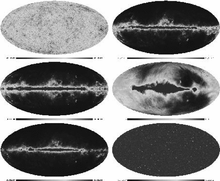
Figure 1: Simulated components at 30 GHz. We show (from up-left to bottom-right,) CMB, thermal dust, free-free, synchrotron, rotational dust and SZ. The maps are in $\Delta T/T$ thermodynamic temperature units.

In order to test the capabilities of the SMHW to detect point sources, we have simulated a data set like the one expected from the Planck mission. We have ten all-sky maps –one for each Planck channel– at nine different frequencies. In Table 1 we show the pixel sizes, antenna FWHMs, HEALPix $N_{\rm side}$ parameters and the expected Planck noise levels (which is assumed to be Gaussian and pure stationary white noise) for all the channels that we have used in the present work. The simulations include PS emission, CMB, Galactic foregrounds (thermal dust, free-free, synchrotron) and SZ (see Fig. 1) as well as instrumental white noise. In Fig. 2 the ten sky maps are shown, and in Table 2 the RMS values for all the components are presented.

The foreground due to the thermal dust emission have been simulated using the data and the model provided by Finkbeiner et al. (1999). That emission is modeled by two gray-bodies with different temperatures from point to point: a hot one with a mean dust temperature of ${T_{D}}^{hot}\simeq 16.2$K and an emissivity $\alpha^{hot}\simeq 2.70$, and a cold one with a mean ${T_{D}}^{cold}\simeq 9.4$K, and $\alpha^{cold}\simeq 1.67$.

Free-free emission is poorly known. Present experiments such as SouthernH-$\alpha$ Sky Survey (SHASSA, Reynolds & Haffner, 2000) and the Wisconsin Halpha Mapper project (WHAM, Gaustad et al. 2001) will provide maps of $H_{\alpha}$ emission that could be used as a template for this emission. At the moment this work was done, free-free maps were not available. We have chosen the idea proposed by Stolyarov et al. (2002) to simulate this component assuming that a $60\%$ of the signal is a thermal dust correlated component, whereas the rest of the emission is uncorrelated (to simulated this uncorrelated component, the flipped thermal dust map is used as template).

Synchrotron emission simulations have been done using the all-sky templates given by Giardino et al. (2002). These maps are an extrapolation of the 408 MHz radio map of Haslam et al. (1982), from the original $1^{\circ}$ resolution. A power law for the power spectrum with an exponent of $-3$ has been assumed. We include in our simulations the information on the spectral index variation as a function of electron density in the Galaxy. This spectral indices template have been done combining the 408 MHz map with the Jonas et al. (1998) one at 2326 MHz and the Reich & Reich (1986) map at 1420 MHz and was done also by Giardino et al. (2002).

Although the results of this paper are given for simulated sky maps where only the previous Galactic emissions are included, we have tested how the presence of rotational dust (Draine & Lazarian 1998) could modify the PS catalogue. Rotational dust emission could be important at the lowest frequencies (30 and 44 GHz), where it could be around ten times greater than the all-sky free-free emission. This emission is strongly correlated with the thermal dust one, through the neutral hydrogen column density ($N_{H}$):

$${I(\nu)}_{\textrm{rot}}=f(\nu)N_{H},\hskip 14.22636pt{I(3000~{}{\rm GHz})_{\textrm{thermal}}}=aN_{H},$$

where $f(\nu)$ is the frequency dependence of the emissivity predicted by Draine & Lazarian (1998) and $a$ is the correlation between the $21$cm emission and the infrared dust one. We adopt the correlation proposed by Boulanger & Pérault (1988):

$$a\approx 0.85\times 10^{-14}{\rm Jy~{}sr}^{-1}{\Big{(}\frac{H~{}\textrm{atoms}}{\textrm{cm}^{-2}}\Big{)}}^{-1}.$$

Therefore, the rotational dust emission is simulated from the thermal one through the equation:

$${I(\nu)}_{\textrm{rot}}=a^{-1}f(\nu){I(3000~{}{\rm GHz})_{\textrm{thermal}}}.$$

The Sunyaev-Zel’dovich (SZ) effect emission have been developed following the model proposed by Diego et al. (2001). These simulations assume a flat $\Lambda$CDM Universe with $\Omega_{m}=0.3$ and $\Omega_{\Lambda}$ = $0.7$. The CMB signal have been simulated for the same Universe, using the $C_{\ell}$ generated with the CMBFAST code (Seljak & Zaldarriaga, 1996).

Finally, the extra-galactic point source (PS) simulations have been performed following the model of Toffolatti et al. (1998) assuming the above adopted cosmological model. Two main PS populations are assumed. At low and intermediate frequencies (from 30 to $\sim 300$ GHz) flat spectrum sources (QSOs, blazars and AGN) dominate bright source counts (i.e., at $S\sim$ 50$\div$100 mJy). This is a model prediction, given that only few data are currently available in this frequency range. On the other hand, the model counts of Toffolatti et al. have been very precisely confirmed by independent observations (CBI, Mason et al., 2002; VSA, Taylor et al., 2002) and, moreover, by the full sky sample of extragalactic sources released by the WMAP satellite (Bennett et al., 2003). At frequencies $\nu\sim 300$ GHz, number counts of extragalactic sources are dominated by dusty galaxies. High redshift spheroids and elliptical galaxies in the phase of rapid star formation and low redshift starburst and normal spiral galaxies. The model number counts of Toffolatti et al. (1998) are still assumed, albeit the new data by SCUBA and MAMBO surveys at sub–mm/mm wavelengths are indicating a greater slope of differential counts at fluxes of a few mJy.

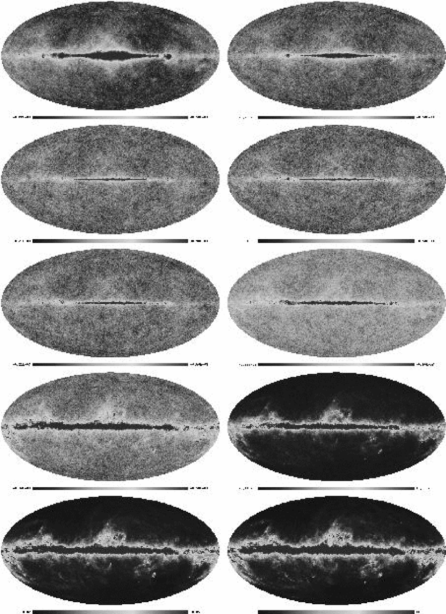
Figure 2: Simulated all-sky Planck maps. The frequencies are (from up-left to bottom-right): 30, 44, 70, 100(LFI), 100(HFI), 143, 217, 353, 545 and 857 GHz. All the maps are filtered with a Gaussian beam and noise have been added following the RMS levels of Table 1. They are in $\Delta T/T$ thermodynamic temperature units.

3 The method

The proposed PS detection method is composed of several pieces. Its basic pillar is the Spherical Mexican Hat Wavelet (SMHW), that is used to convolved the analysed signal at different scales in order to achieve a cleaned map; we describe the SMHW in Subsection 3. Because the expected pixelization for the Planck maps is the HEALPix scheme, we have developed the method in this framework; this implies some peculiar characteristics that will be discussed in Subsection 4. The proposed method is not simply a convolution of the maps with the SMHW, there are several steps in the algorithm that are commented in Subsection 6. One of the important steps in the PS catalogue estimation is the detection criterion: we will discuss about this topic in Subsection 3.4.

3.1 The tool: Spherical Mexican Hat Wavelet

Figure 3: We show the SMHW $a_{lm}$ for $R=42$ arcmin (the largest scale used in this work). In addition, we plot (dashed line) the difference between the SMHW $a_{lm}$ and the MHW one, 50 times magnified.

The SMHW has been used recently to study the CMB Gaussianity/Non-Gaussianity in the COBE-DMR data (Cayón et al. 2002) and in Planck simulations (Martínez-González et al. 2002). The extension of the plain Mexican Hat Wavelet (MHW) to the sphere (like the spherical extension of any wavelet) is not an obvious issue. The stereographic projection has been suggested by Antoine & Vanderheynst (1998) as the most suitable manner to do this extension, since the MHW properties are kept and at the small angle limit tends to the MHW. A graphical explanation of such extension can be found in Martínez-González et al. (2002), here we just remark the expression for the MHW and the SMHW. The MHW is given by Eq. (1) and it satisfies the compensation ($\int d\vec{x}\,\Psi=0$), admissibility ($C_{\Psi}=(2\pi)^{2}\int_{0}^{\infty}dk\,k^{-1}{\Psi}^{2}(k)<\infty$, where $\Psi(k)$ is the Fourier transform of $\Psi(x)$) and normalization ($\int d\vec{x}\,{\Psi}^{2}=1$) properties that define a wavelet (see Martínez-González et al. 2002 for details):

$$\Psi(x)=\frac{1}{\sqrt{2\pi}}\frac{1}{R}\Big{[}2-\big{(}\frac{x}{R}\big{)}^{2}\Big{]}e^{-\frac{x^{2}}{2R^{2}}},$$ (1)

in that expression $R$ is the MHW scale and $x$ is the distance. Through the stereographic projection, we deal with the SMHW expression:

$$\Psi_{S}(y,R)=\frac{1}{\sqrt{2\pi}N(R)}{\Big{[}1+{\big{(}\frac{y}{2}\big{)}}^{2}\Big{]}}^{2}\Big{[}2-{\big{(}\frac{y}{R}\big{)}}^{2}\Big{]}e^{-{y}^{2}/2R^{2}},$$ (2)

where $R$ is the scale and $N(R)$ is a normalization constant:

$$N(R)\equiv R{\Big{(}1+\frac{R^{2}}{2}+\frac{R^{4}}{4}\Big{)}}^{1/2}.$$ (3)

The distance on the tangent plane is given by $y$ that is related to the latitude angle ($\theta$) through:

$$y\equiv 2\tan\frac{\theta}{2}.$$ (4)

Given the SMHW, a signal on the sky $f(\vec{n})$ (being $\vec{n}$ a vector in the projection plane) can be analysed, obtaining the wavelet coefficients:

$$w(\vec{n},R)=\int d\Omega^{\prime}\,f(\vec{n}+\vec{n}^{\prime})\Psi_{S}(\theta^{\prime},R).$$ (5)

where

$$\vec{n} \equiv 2\tan\frac{\theta}{2}(\cos\phi,\sin\phi),$$ (6)

$$\vec{n^{\prime}} \equiv 2\tan\frac{\theta^{\prime}}{2}(\cos\phi^{\prime},\sin\phi^{\prime})$$ (7)

If the signal $f(\vec{n})$ is a PS with a Gaussian shape, then the wavelet coefficient at the PS position is a known function of the antenna width ($\sigma_{a}$), the SMHW scale ($R$) an the PS intensity ($I$).

For the SMHW scales used in this work (smaller than $1^{\circ}$) the SMHW can be described by the plain MHW with good accuracy. In Fig. 3 we have plotted (solid line) the spherical harmonic coefficients ($a_{lm}$) of the SMHW at the largest scales used in our work ($R=42$ arcmin); we also plot (50 times magnified) the difference between these coefficients and the Fourier coefficients that describe the MHW at the same scale (dashed line). This implies that, for the typical cases studied in this work, we consider the MHW and the SMHW coefficients to be the same for all practical purposes. Therefore, for the optimal scale determination through the plane projection (see next Section) and for the analytical expression relating the wavelet coefficient at the scale $R$ with the beam dispersion ($\sigma_{a}$) and the point source amplitude ($I$) (see Eq. 8), the MHW is used. On the other hand, all-sky convolutions are performed using the SMHW.

$$w(R)=2\sqrt{2\pi}IR\frac{(R/\sigma_{a})^{2}}{(1+(R/\sigma_{a})^{2})^{2}}.$$ (8)

We are interested in detecting PS in wavelet space rather than real space because, by convolving the map with the SMHW, we can increase the signal-to-noise ratio of the sources. This increment is characterised by the amplification factor:

$$A=\frac{w(R)/\sigma_{w}(R)}{I/\sigma_{m}},$$ (9)

where $\sigma_{w}(R)$ is the dispersion of the wavelet coefficients and $\sigma_{m}$ is the dispersion of the analysed signal. If we assume that the background is an statistically homogeneous and isotropic random field with zero mean, and taking into account that its variance is given by:

$${\sigma^{2}}_{w}(R)=<w(\vec{n},R)^{2}>-<w(\vec{n},R)>^{2},$$ (10)

then it is straightforward to show that:

$${{\sigma}^{2}}_{w}(R)\propto\int d\,qq\,P(q)|\tilde{\Psi}(qR)|^{2}.$$ (11)

where $P(q)$ is the power spectrum of the analysed signal and $\tilde{\Psi}(qR)$ is the Fourier transform of the MHW.

The amplification reaches its maximum value at the optimal scale, $R_{o}$ (see Vielva et al. 2001a for a detailed description). Taking into account Eqs. (8), (9) and (11), we can calculate the optimal scale from the data itself ($C_{\ell}$, $\sigma_{m}$ and $\sigma_{a}$). Once the PS position is determined (by the location of the maxima in wavelet space), we can estimate the PS intensity by calculating the wavelet transform at each selected location at several scales, in order to compare these values with the theoretical curve (Eq. 8). We can define a $\chi^{2}$ at each selected position $\vec{n}$:

$$\chi^{2}(\vec{n})=\sum_{i,j}({w_{\vec{n},R_{i}}}^{t}-{w_{\vec{n},R_{i}}}^{e})V_{ij}^{-1}({w_{\vec{n},R_{j}}}^{t}-{w_{\vec{n},R_{j}}}^{e}),$$ (12)

where $V_{ij}$ represents the wavelet coefficients covariance matrix element between scales $i$ and $j$ (calculated from the data) and ${w_{\vec{n},R_{i}}}^{t}$ and ${w_{\vec{n},R_{i}}}^{e}$ are the theoretical (Eq. 8) and experimental values of the wavelet coefficients at scale $R_{i}$ and location $\vec{n}$. We use four different scales to perform the multiscale fit (see Vielva et al 2001a for a detailed description of the covariance matrix and the multiscale fit).

3.2 The framework: HEALPix

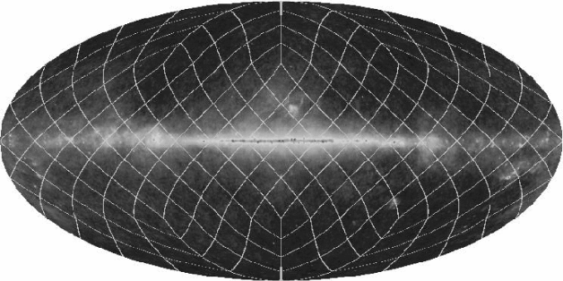
Figure 4: Sky division in father pixels ($N_{\rm side}$ = 4). The optimal scale is determine in each one of these areas.

The Hierarchical Equal Area and iso-Latitude Pixelization (HEALPix) have been suggested by Gorski et al. (1999) as the most suitable sphere pixelization since it allows hierarchical tree structure and fast spherical harmonics transform. These two properties give us great advantages in order to deal with the PS detection. First of all, the hierarchical structure allows to identify quickly pixels in the sphere, what is specially relevant for large data sets. We have used this characteristic to determine the optimal scale in different patches of the sky with low CPU time consumption. As it is shown in Vielva et al. (2001a) the determination of the optimal scale is essential in order to achieve the largest amplification. The simulated Planck maps show strong differences from one direction to another, for example, at 30 GHz, we can see synchrotron and free-free structure at the Galactic plane, but the CMB emission dominates at high Galactic latitude. Hence, a global optimal scale is, clearly, far from being optimal. We have divided the sky in areas that coincide with the HEALPix pixels at $N_{\rm side}$ = 4 resolution (see Fig. 4). We have chosen this resolution because the pixels (hereafter we refer to these as father pixels) have a characteristic size $\sim 10^{\circ}$, close to the patch size adopted by Vielva et al. (2001a). One can think of alternatives to determine the optimal scale. For example, we have tested to determine it in iso-latitude bands, but we lose precision in the optimal scale determination, especially at low Galactic latitude.

To calculate the optimal scale the $C_{\ell}$ of the signal are needed. The $C_{\ell}$ calculation of each father pixel on the sphere is, in practice, an unrealizable task: there are 192 areas and, for each one of them we need to calculate the $a_{lm}$ sets with good accuracy up to $l_{max}=3N_{\rm side}-1$. To determine the $a_{lm}$ set of an isolated region of the sky is a difficult issue, we can fill out with zero values all the pixels outside the particular zone and to proceed as an all-sky $a_{lm}$ calculation (only the large scales are mislead, but it is not important since the relevant information to determine the optimal scale is at the smallest scales). Another alternative is to use orthonormal basis for a given cut sky (Mortlock et al. 2002). To calculate these bases for all the father pixels is a very slow process (it scales as $O({l_{max}}^{6})$ for each father pixels); however, once the calculation is done, the basis can be stored. Unfortunately, as the authors point out, the required space to store these bases scales as $O({l_{max}}^{4})$. Hence, this alternative is inadequate for the Planck resolutions.

To solve this issue, we project each father pixel in a plain tangent squared patch, filling with zero those pixels of the patch outside the projected image (see Fig. 5). Afterwards, we can calculate the optimal scale through the power spectrum of each particular area using the Fourier transform.

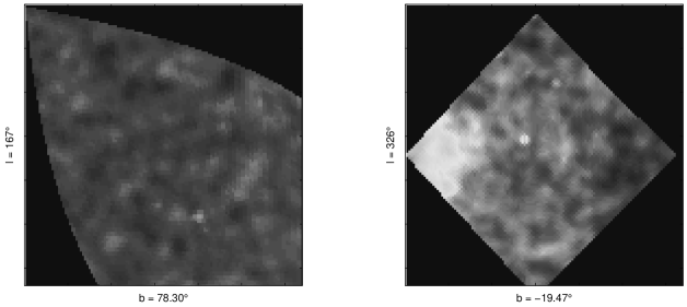
Figure 5: We show the projections of two father pixels in squared plain patches. The left one represents one of the four father pixels at the north pole, whereas the one in the right hand shows a father pixel near the Galactic plane. The error in the optimal scale determination in the squared patch due to the projection is less than $5\%$.

This approximation makes the computation of optimal scale easy and fast, but we are making an error in the optimal scale determination due to the projection. However, we have tested that the mean error all over the sky is less than $5\%$, when we compare with the optimal scale determination through the spherical analysis. This implies an amplification (flux limit) which is $\approx 1\%$ lower (greater) than the one obtained through the right spherical procedure.

3.3 The algorithm

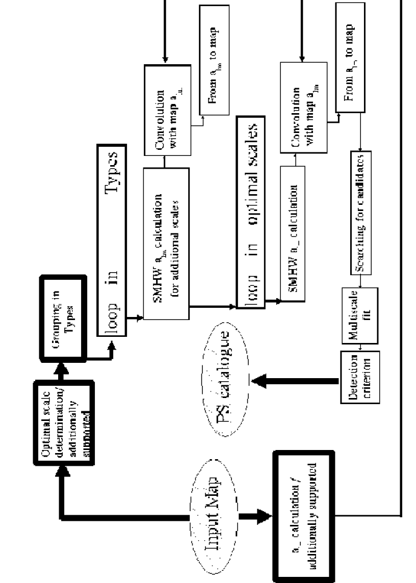
Figure 6: Schematic algorithm of the process. See text for details.

We present the different steps that constitute the PS detection algorithm. Given a map to be analysed we need to estimate the optimal scale in each sky area, in the way indicated in the previous Subsection. Together with the optimal scale, we need other SMHW scales, in order to perform the multiscale fit. We call these scales adjacent scales. Here we need to make another simplification in order to reduce the CPU time. If we make the adjacent scale choice completely dependent on the optimal scale value, we finally have 4 different SMHW $a_{lm}$ sets for each optimal scale. We must convolve the map with each one of these scales and then a transformation from harmonic space to wavelet space is required to detect the PS. This last process (spherical harmonic transform) is the major contribution to the CPU time consumed. We need to reduce these calculations as much as possible.

In order to reduce the CPU time, we group the optimal scales in three types. All optimal scales belonging to the same type have the same adjacent scales. This reduces enormously the CPU time, making the process viable.

• type I: the optimal scale is lower than half a pixel. This occurs when the dominant background is due to foregrounds with a variation scale larger than the PS one (i.e. the beam width) and with a very high emission. This behaviour can be found close to the Galactic plane and in some high Galactic emission zones. Due to the pixelization, we can not use SMHW scales too small, hence a lower limit must be imposed to avoid discrepancies between the wavelet coefficients and its theoretical value (Eq. 8). For that reason, we assign the value $R_{o}\equiv 0.5P_{s}$ to those father pixels belonging to this type I, where $P_{s}$ is the pixel size (see Table 1). In this case, the three adjacent scales will be greater than the optimal one.

• type II: the optimal scale is smaller than the beam width but larger than half a pixel. This occurs in regions where the major background is a signal with a variation scale close to the PS one: sky areas dominated by the CMB emission, with a low contribution due to instrumental noise and poor resolution . This also happens for regions with a moderate synchrotron or free-free emission which nonetheless is the dominant one. Most of the optimal scales used in this work belong to this type. In this case the adjacent scales are also greater than the optimal one, but the $R_{o}$ has not a minimum value.

• type III: the optimal scale is close to the beam width. The signal components with variation scales larger than the PS one are dominant (Galaxy components), but their emission is lower than in previous types. In addition, the instrumental noise dominates over the CMB emission. This happens at very high Galactic latitudes in dust-dominated channels. One of the adjacent scales is smaller than $R_{o}$, whereas the other two are greater.

The wavelet coefficient at the scales that come from the previous division are well described by the theoretical curve (Eq. 8). Only those coefficients at scales equal or lower than the pixel size and at high latitude (where the HEALPix pixels have an elongated shape) are slightly affected by pixelization problems. However, as Fig. 7 shows, the errors for most of the cases are less than $5\%$ and close to zero for the rest of the situations (intermediate and low latitudes and scales larger than the pixel size).

Figure 7: Deviation of the wavelet coefficients from the theoretical curve (Eq. 8) for several Galactic latitudes. The plots represent (from up-left to bottom-right) the 44, 100 (LFI), 143 and 545 GHz.

Once the $a_{lm}$ sets at the adjacent scales are calculated, the SMHW convolution of the map is performed for these scales. We want to remark that the SMHW convolution is performed in all the sky, not only on those father pixels that belong to the same type: it is a spherical convolution. We anti-transform the convolved $a_{lm}$ to get the wavelet coefficients of the sky maps. To do that efficiently, we use another of the HEALPix properties: the iso-latitude pixelization. A map in HEALPix has 4$N_{\rm side}$ - 1 iso-latitude rings, for each one of these rings, we calculate the Legendre polynomials (that only depend on the declination angle). Using these functions we can calculate the harmonic transform of each ring at the same time for the three adjacent scales.

Afterwards, we calculate the SMHW $a_{lm}$ sets of each optimal scale of the peculiar type. We convolve the map and anti-transform the convolved $a_{lm}$ set to the wavelet space and search for maxima in the optimal scale wavelet coefficients map on these father pixels belonging to the specific optimal scale.

At this point, we want to comment about a problem related with the estimation of the mean value of the wavelet coefficients maps. The maps that we are analysing have zero mean and the wavelet transform keeps the mean value. However, because we are searching for maxima only on those father pixels with a given optimal scale, the wavelet coefficients set on those father pixels have not zero mean (the zero mean is a global property). In other words, the zero level is mislead. This is an important problem at high frequency channels (from 353 GHz to 857 GHz), where the Galactic contribution is so high that the mean is completely dominated by it: the SMHW convolution is not able to remove sufficiently the Galactic contribution (near the Galactic plane). It implies an offset in the wavelet coefficients and also in the PS amplitudes. To solve this problem, we recalculate the zero level of each wavelet coefficients set. The bias in the amplitude estimation is not removed completely; however, as it can be seen in the next Section it is not important and it can be determined.

Once the maxima are located we perform a multiscale fit using the four scales (the optimal and the 3 adjacent ones) to estimate the PS amplitude. We repeat this algorithm for all the optimal scales in each type and for all the types. In Fig 6 we show an schematic diagram of the algorithm.

The process takes 72 hours for the worse case: the 857 GHz map, $N_{\rm side}$ = 2048. We have run the code in a Compaq HPC320 (Alpha EV68 1 GHz processor) and it requires 4 GB of RAM memory. The $a_{lm}$ map estimation takes $\sim$ 8 hours, since we need to have scale information up to the highest resolution $l=3N_{\rm side}-1$. The optimal scale determination is really fast ($\sim 15$ minutes). The rest of the time is due to transformations from harmonic domain to wavelet space (we have used 17 different optimal scales for the 857 GHz map). The CPU time goes, basically, as $O(N_{R_{o}}{N_{\rm pix}}^{3/2}log(N_{\rm pix}))$, where $N_{\rm pix}$ is the number of pixels in the map ($N_{\rm pix}=12{N_{\rm side}}^{2}$) and $N_{R_{o}}$ is the number of optimal scales.

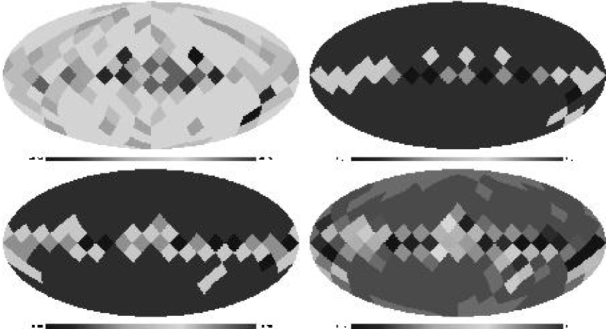
Figure 8: We present the optimal scale maps of four channels: 44 GHz (top-left), 100 GHz LFI (top-right), 217 GHz (bottom-left) and 545 GHz (bottom-right). They are in antenna width ($\sigma_{a}$) units (see Table 1).

3.4 The detection criterion

To define a detection criterion is an important task in the field of the PS detection. A good detection criterion should be robust, efficient and unbiased. The robustness property implies that the criterion must not depend on the specific data characteristics. It must be efficient in order to detect the maximum number of true sources with the minimum error (both, in the amplitude and position determination).

Up to this point, we just are able to provide cleaned maps of the sky with good PS amplitude estimation obtained from a multiscale fit. To decide which one is a real source from the map of maxima is an issue that is outside the scope of this paper. There are several works in the literature dealing with this problem. One of them defines a detection criterion for the maxima based on the acceptation region (using the Amplitude-Curvature space) given by the Neyman-Pearson lemma (Barreiro et al. 2003); results are presented for backgrounds described by Gaussian random fields. Other authors have suggested the False Discovery Rate (FDR) method (Hopkins et al. 2002) or a Bayesian approach to detect and characterize the maxima (Hobson & McLachlan 2002).

In general the application of detection criterions having the desirable properties mentioned above is, in practice, very complicated. Moreover, they have been applied to situations for which the background has very simple and well known statistical properties. Even more, they have been tested on small data sets. For the Planck case the situation is very different: some of the backgrounds have complex statistical properties and the data sets are very large. The results presented in the next Section are obtained assuming a detection criterion that is able to get a catalogue with a maximum percentage ($5\%$) of spurious detection, where spurious is a detection with an error (in absolute value) in the amplitude estimation larger than $50\%$ (see Vielva et al. 2001a for details). This simple detection criterion assumes that the simulations for the different components describe well enough the main statistical properties of the real ones. Hence, in practice, this exercise gives us a flux limit which will be used as a threshold for the real case. Above this threshold, the percentage of spurious detections will be expected to be $\leq 5\%$.

We are working on a detection criterion for the Planck data that takes into account multi-frequency information as well as simple PS distribution features. Results will be presented in a future work.

4 Results

Frequency (GHz)	#	Min Flux (Jy)	$\bar{E}(\%)$	$\bar{b}(\%)$	Galactic Cut(deg)	$N_{R_{o}}$	Completeness (%)
857	27257	0.48	17.7	-4.4	25	17	70
545	5201	0.49	18.7	4.0	15	15	75
353	4195	0.18	17.7	1.4	10	10	70
217	2935	0.12	17.0	-2.5	7.5	4	80
143	3444	0.13	17.5	-4.3	2.5	2	90
100(HFI)	3342	0.16	16.3	-7.0	0	4	85
100(LFI)	2728	0.19	17.0	-2.4	0	4	80
70	2172	0.24	17.1	-6.7	0	6	80
44	1987	0.25	16.4	-6.4	0	9	85
30	2907	0.21	18.7	1.2	0	7	85

Table 3: PS catalogue obtained from the Planck data using the SMHW method proposed. In column 2 we print the number of detections above the flux limit given in column 3 with a maximum $5\%$ of spurious detections. The mean error (in absolute value) is shown in column 4, whereas the mean bias is in column 5. The Galactic cut below which no detection is available is shown in the sixth column. The number of optimal scales appears in the column number 7 and the completeness of the catalogue in the last one.

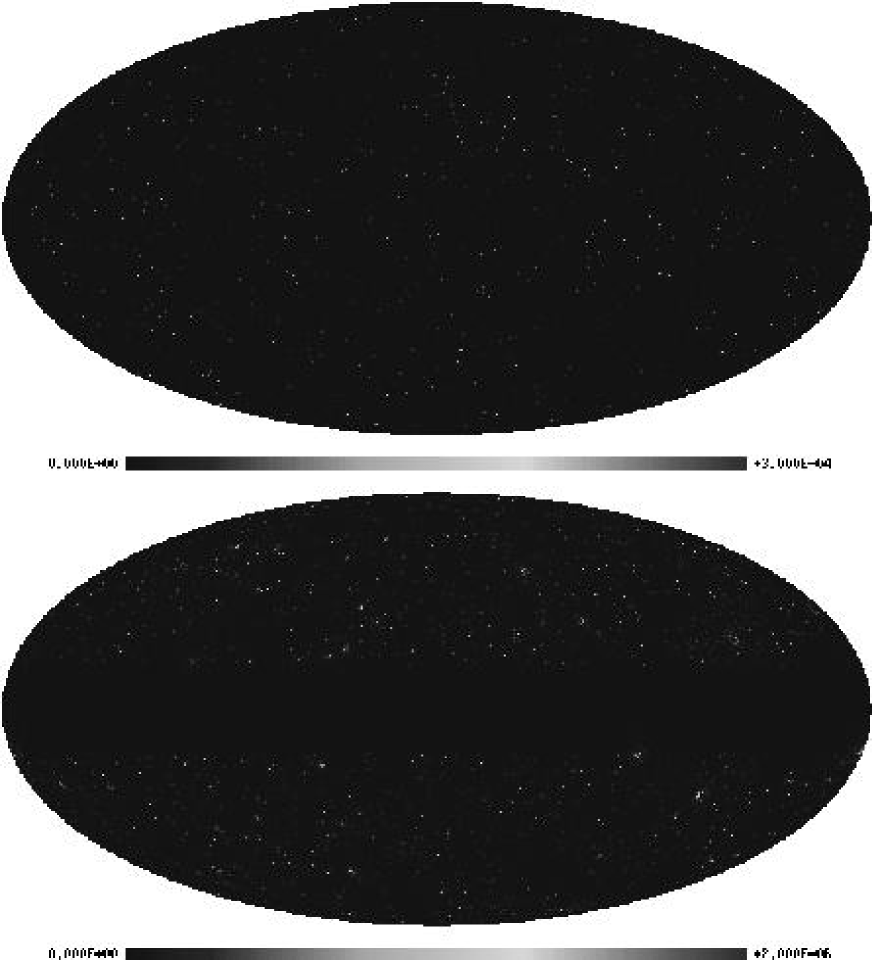
Figure 9: Recovered point source maps. The frequencies are 44 GHz and 545 GHz. The maps are filtered with a Gaussian beam (see Table 1).

			$85\%$				$90\%$				$95\%$				$99\%$
Freq	#	flux	$\bar{E}$	$\bar{b}$	#	flux	$\bar{E}$	$\bar{b}$	#	flux	$\bar{E}$	$\bar{b}$	#	flux	$\bar{E}$	$\bar{b}$
(GHz)	(Jy)		(%)	(%)	(Jy)		(%)	(%)	(Jy)		(%)	(%)	(Jy)		(%)	(%)
857	12763	0.78	11.1	1.1	10001	0.91	9.7	1.5	6763	1.19	7.8	1.7	2816	2.00	4.7	1.1
545	3668	0.60	16.3	5.7	2806	0.72	14.5	6.4	1844	0.91	11.7	6.3	421	2.22	4.9	2.8
353	2233	0.28	13.4	6.2	1718	0.33	12.0	6.2	1177	0.42	10.0	6.0	294	0.94	4.8	3.1
217	2288	0.15	14.5	1.0	1850	0.18	12.9	2.6	1440	0.22	11.1	3.4	779	0.34	7.8	3.8
143	3444n	0.13n	17.5n	-3.3n	3444n	0.13n	17.5n	-3.3n	2576	0.17	14.2	-0.9	1776	0.23	11.4	0.2
100	3342n	0.16n	16.3n	-7.0	2727	0.20	13.4	-4.5	2078	0.26	10.9	-2.6	1224	0.40	7.5	-0.7
(HFI)
100	2370	0.22	15.2	-0.6	1768	0.29	12.7	1.6	1323	0.37	10.4	3.1	635	0.65	743	4.3
(LFI)
70	2076	0.25	16.4	-5.9	1399	0.35	12.3	-2.3	867	0.51	8.2	0.2	554	0.70	6.2	0.6
44	1987n	0.25n	16.4n	-6.4n	1489	0.33	13.2	-3.8	1092	0.43	10.6	-2.4	608	0.67	7.5	1.3
30	2706	0.22	18.1	1.7	2264	0.26	15.4	3.7	1921	0.30	14.3	3.9	1099	0.45	10.6	3.5

Table 4: PS catalogues for different completeness levels ($85\%$, $90\%$, $95\%$ and $99\%$). For each completeness level we show the number of detections, the minimum flux and the mean error and bias. The letter ’n’ means that the results on that column are the same than in the previous Table.

Applying the method described in Section 3 to the simulations shown in Section 1, we are able to obtain all-sky Planck PS catalogues. The catalogue is presented in Table 3.

The total number of PS detected is given in the second column. We are just able to detect those sources in the tail of the PS distribution (we comment more about this below). The minimum fluxes achieved at each frequency are shown in the third column. At intermediate frequencies we are able to reach lower fluxes because it is the microwave window where Galactic emission is lower. The 100 GHz HFI channel is specially important for the PS detection, since it is expected to have a low instrumental noise. In columns four and five the mean error, $E(\%)$, and bias, $b(\%)$, are presented, where:

$$\bar{E}(\%) = \sum_{\vec{n}}\frac{|I_{\vec{n}}-\tilde{I}_{\vec{n}}|}{I_{\vec{n}}}100$$ (13)

$$\bar{b}(\%) = \sum_{\vec{n}}\frac{I_{\vec{n}}-\tilde{I}_{\vec{n}}}{I_{\vec{n}}}100,$$ (14)

being $I_{\vec{n}}$ the PS intensity at location ${\vec{n}}$ and $\tilde{I}_{\vec{n}}$ the method estimation. The mean error is between $\approx 16-19\%$, whereas the bias behaviour changes along the frequency range. One of the reasons for that change arises from the fact that we perform a zero-level recalculation of the wavelet coefficients at high frequency Planck channels. The new zero-level is not perfectly estimated and, hence, the PS amplitudes are systematically underestimated or overestimated. However, this kind of bias can be taken into account and it can be corrected in the PS amplitude estimation. Due to the Galactic emission, there are latitudes where the PS detection is not possible. We show this in column six. At low and intermediate frequencies the Galaxy is not a problem, but, obviously at higher frequencies it becomes a handicap. In column seven we present the number of optimal scales needed in the algorithm. Since the homogeneous CMB emission is the dominant contribution at intermediate frequencies, the number of required optimal scales at these channels is lower than in the other due to the gradient pattern for the Galactic emission. In Fig 8 we plot, as an example, the optimal scale maps for the 44 , 100 (LFI), 217 and 545 GHz channels. Finally, in column eight we represent the completeness percentage (above the minimum flux and outside the Galactic cut) that the detected catalogue represents. The completeness percentage is $\sim 80\%$ for low and intermediate frequency channels and it decreases for high ones. In Figs. 9 (44 and 545 GHz) we show the PS catalogue maps, where the areas without PS detection can be seen for channels at high frequency

Figure 10: Tails PS distribution function - $N(F)dF$- for the input PS maps (dark histograms) and the residual ones (light histograms) obtained by subtracting the recovered PS catalogue show in Table 3 from the simulated PS.The frequencies are (from up-left to bottom-right): 30 GHz, 100 GHz (LFI), 353 GHz and 857 GHz.

We want to remark that these results have been obtained without including the rotational dust emission. If this emission is present in the simulations, the 30 and 44 GHz results change, whereas the results for the rest of the channels are the same. In particular, at 30 GHz, the number of detected PS is 1809 and the minimum flux is 0.41 Jy; in addition, 11 optimal scales are required. For the 44 GHz channel 1055 PS are detected and 0.51 Jy is the minimum flux that we are able to achieve (the number of optimal scales is the same).

An interesting question is to study the different completeness catalogues that can be achieved with the method. We present in Table 4 the complete catalogues at $85\%$, $90\%$, $95\%$ and $99\%$ levels. For 30 GHz and 44 GHz channels the completeness catalogues at $85\%$ are the same that the ones in Table 3, whereas the for 143 GHz channel the catalogue in Table 3 represents a $90\%$ complete one. Obviously as the completeness level increases, the number of detected PS is lower and the flux limit achieved is higher. However, the accuracy of the catalogues is better as the mean errors and bias show.

If we subtract the recovered PS catalogues from the input PS maps, we obtain residual PS maps, with RMS values lower than the input ones (see Table 5). The power spectrum of a Poisson distribution in the sky of PS is flat and is proportional to the $\textrm{RMS}^{2}$ and therefore the power spectra of the residual PS maps are correspondingly reduced by a factor $(\textrm{RMS}_{\textrm{input}}-\textrm{RMS}_{\textrm{residual}}/\textrm{RMS}_{\textrm{input}})^{2}$.

Frequency	Input PS	Residual PS
(GHz)
857	$1.96\times 10^{-2}$	$1.60\times 10^{-2}$
545	$1.91\times 10^{-4}$	$1.53\times 10^{-4}$
353	$1.39\times 10^{-5}$	$1.17\times 10^{-5}$
217	$3.45\times 10^{-6}$	$2.41\times 10^{-6}$
143	$3.54\times 10^{-6}$	$1.65\times 10^{-6}$
100 (HFI)	$5.41\times 10^{-6}$	$1.30\times 10^{-6}$
100 (LFI)	$5.79\times 10^{-6}$	$1.54\times 10^{-6}$
70	$7.43\times 10^{-6}$	$2.16\times 10^{-6}$
44	$1.08\times 10^{-5}$	$3.15\times 10^{-6}$
30	$1.54\times 10^{-5}$	$4.56\times 10^{-6}$

Table 5: The PS RMS values (in $\Delta T/T$ units) for the simulated Planck channels are presented. In the second column we show the RMS of the input PS maps, whereas in the third one it is shown the RMS after the detected PS (the ones in Table 3) are subtracted. All the maps have been convolved with the beams.

As we commented before, the detected PS belong to the tail of the PS distributions. This can be seen in Fig. 10 where we plot the input and residual PS tail distribution for the catalogue of Table 3. Only the brightest sources are removed from the map. However, removing these brightest sources is a critical issue if we want to apply this PS detection method in combination with all-component separation ones such as MEM or Fast Independent Component Analysis (FastICA). These methods need to assume that the PS distribution is Gaussian (more realistic PS distributions require non-Gaussian probability distribution function) in order to deal with the PS emission. Clearly, this assumption is closer to reality if the brightest sources are removed. Moreover, as the RMS PS decreases, this component is less important (see Vielva et al. 2001b).

The last result we comment is that the recovered PS catalogues provide spectral information of the PS populations, since several PS can be detected at different channels. Therefore we can study the frequency dependence of the PS emission, this can be useful to study the physical processes that generate such emission. This is important at all Planck channels, because there is a lack of information at these frequencies. It is particularly relevant at intermediate Planck frequencies, where the knowledge of the different PS populations is really poor. We can follow 57 sources in the whole Planck spectral interval, 1585 can be seen from 30 GHz to 100 GHz channel, 942 from 143 GHz to 353 GHz and 2231 from 353 GHz to 857 GHz. In Fig. 11 we plot some of these sources.

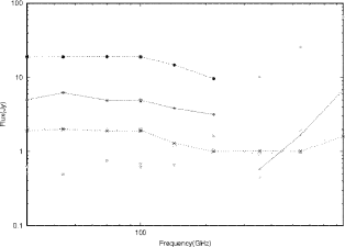
Figure 11: Spectral behaviour for some of the detected sources found in coincidence at several channels.

If we focus on spectral intervals small enough to assume a power law for the PS emission, we can estimate the spectral indices:

$$F=F_{o}\Big{(}{\frac{\nu}{\nu_{o}}}\Big{)}^{\alpha},$$ (15)

where $\alpha$ is the spectral index that will define the different PS populations.

In Table 6 we give an estimation of the spectral indices for different frequency ranges (and using the catalogue described in Table 3). By fitting the PS estimated amplitudes, we can determine the $\alpha$ parameter that appears in columns 6, 7 and 8 whereas the input (simulated) values are shown in columns 3, 4 and 5. The mean errors are presented in the last column. For spectral indexes close to zero – i.e. indexes of sources associated to QSOs, blazars and AGNs, whose emission is dominated by the nuclear activity – we give the absolute error whereas relative errors are provided for typical spectral indexes of sources whose emission is dominated by cold dust at microwave frequencies (e.g., ultraluminous IRAS galaxies, high redshift spheroids and starburst/interacting galaxies). From Table 6 it is apparent that we are able to well recover the average input spectral index in every frequency range of the Planck experiment.

A handful of sources (57) are detected in all channels. Albeit this is a small number if compared to the ones in the complete catalogues, it will allow to follow the spectral behaviour in a range in which should appear the steepening of the synchrotron spectrum due to electron energy losses. This will help to establish, e.g., the synchrotron age of the source, the relative importance of the free–free emission, etc.

Moreover, the high number of detected sources in at least two/three nearby channels allows us to single out the different source populations dominating the counts of bright sources at different frequencies. On one side, by the HFI channels, it will be possible to define much better the spectral properties of the cold dust emission. This information – complemented by the one coming from the surveys of the Herschel satellite at higher frequencies – shall help to fix the temperature of the cold and warm dust components in different sources. Therefore, it should be possible, in principle, to distinguish between high redshift spheroids in the early phase of their star formation and low redshift normal spirals whose emission is mostly dominated by the cold dust spread all over the galaxy.

On the other side, a complete catalogue of approximately a thousand of sources – detected by LFI and mostly associated to AGN – can be released and this will greatly help to better understand the physical processes originating in the nuclear region of a galaxy and the properties of the emitted radiation.

Eventually, a number of inverted spectrum sources should show up at the intermediate Planck channels and this will help to study the relevance in number counts and the spectral properties of such source populations as Gigahertz Peaked (GPS) and Advection Dominated (ADS) sources which currently are very poorly known (see Toffolatti et al 1999).

Channels (GHz)	#	$\alpha_{min}$	$\overline{\alpha}$	$\alpha_{max}$	${\alpha_{min}}^{est}$	${\overline{\alpha}}^{est}$	${\alpha_{max}}^{est}$	Mean Error
857 – 545	4132	-0.11	2.43	3.49	-0.66	2.41	4.41	12.29$\%$
857 – 545 – 353	2231	-0.46	2.16	3.50	-0.52	2.58	3.79	7.13$\%$
353 – 217 – 143	942	-0.91	-0.03	3.08	-2.04	-0.08	3.40	0.17
100 – 70 – 44 – 30	1585	-0.72	-0.14	0.41	-1.01	-0.17	0.63	0.11
44 – 30	1767	-1.46	-0.19	0.74	-2.44	-0.15	2.17	0.31

Table 6: Spectral indices for PS found in coincidence at the channels indicate in column 1. The number of the PS found is given in the second column. Columns 3, 4 and 5 give the minimum, mean and maximum values of the spectral indices as calculated from the input PS. The spectral index estimation is presented in columns 6, 7 and 8. The mean error in the estimation (absolute error for spectral index close to zero are given) is shown in the last column.

5 The case of a non-ideal instrument

We have also tested the influence of realistic asymmetric beams not only in the number of detected point sources, but also in the flux limits achieved and the mean error in the amplitude estimation. This a very important point, since the expected beam shapes for Planck satellite have a asymmetric profiles. A detailed study about the influence of this secondary effect, non-uniform noise distribution and other systematic effects for the detection of point sources, will be presented in a future work. Here we just present the basic procedure to adapt the SMHW method presented in Section 3 to the case where the beam is asymmetric and non-uniform and $1/f$ noises are considered.

Although the SMHW is an isotropic wavelet, it can be also adequate to perform the detection of point sources that show a slight Gaussian asymmetry . This is precisely the situation for the Planck beams, where, due to the scanning strategy, at a given point in the sky, the effective beam is an average of the pure asymmetric antenna over all the possible orientations. This makes the resultant beam more symmetric than the original one. Moreover, we have shown that the SMHW itself is a very promising tool to characterize the effective dispersion ($\sigma_{eff}$) of the realistic beam, by performing a multi-scale analysis of point-like objects in the sky that have been convolved with realistic beams following the expected Planck scanning strategy, (available for the Planck community at the web site http://www.mpa-garching.mpg.de/$\sim$planck/). Thanks to this multi-scale analysis, we can determine the $\sigma_{eff}$ at any direction on the sky. Let us remark here the main results of this study for the case of the largest Planck beam asymmetry: the 30 GHz channel. We have used simulations where realistic beam, non-uniform and $1/f$ ($f_{knee}=100$ mHz) noises are included. The asymmetric beam is close to a Gaussian, with an ellipticity of $\sim 20\%$ with a minor dispersion of 15.47^′. We found that, on average, the $\sigma_{eff}$ (after the scanning strategy) is around 1.39 times the nominal Planck dispersion in this channel.

By comparing the point source catalogue that the SMHW provides in this realistic case, with the one that we would get in the case where an ideal Gaussian beam is used (with an area equal to the one of the real asymmetric beam, that is 1.2 times the nominal dispersion), we show that around 80% of the point sources are still recovered, and the flux limit is just 10% above the one found for the ideal case. The mean error and bias are practically the same in both cases. We want to remark that the discrepancy between the effective beam value average to all the sky, 1.39, that we found for the realistic antenna and the 1.2 value for the ideal case (both in units of the nominal dispersion) arises from the scanning strategy that widens the effective beam in the realistic situation.

6 Conclusions and discussion

We have extended the work done in Vielva et al. (2001a) focused on the detection of PS in simulated microwave flat patches of the sky, to the whole celestial sphere. We have done a spherical analysis using the Spherical Mexican Hat Wavelet that is obtained as an stereographic projection of the plane Mexican Hat Wavelet. This extension implies several new steps in the MHW detection method. First of all, we need to estimate the optimal scale at each area of the sky, in order to achieve the maximum number of detections. To perform the optimal scale determination of the spherical maps is a huge task that involves several transformations (from harmonic domain to wavelet space and viceversa) requires a long CPU time and/or storage space. Using the fact that the HEALPix package allows to identify quickly pixels in the sky, we have done plain projections of HEALPix pixels (at $N_{\rm side}$ = 4) to calculate the optimal scale using Fourier Transform. This approach reduces enormously the CPU time to estimate the optimal scale. We have checked that the error introduced in the optimal scale determination due to the projection is lower than $5\%$. We have tested that the amplification (flux limit) is greater (lower) than $1\%$ the one obtained using the exact value of the optimal scale. A big effort has been also done to reduce the CPU time needed for the harmonic transforms. Whereas the SMHW convolution is done in the harmonic domain, the PS detection is done in wavelet space. In addition, three adjacent scales are required for each optimal one, in order to perform a multiscale fit of the wavelet coefficients to better estimate the PS amplitudes. We have solved this problem by modifying some of the HEALPix package codes to perform several harmonic transformations at the same time using pre-computed Legendre polynomials.

Applying the presented algorithm with the detection criterion based on the simulations (see Subsection 3.4) that is able to produce PS catalogues with a maximum percentage of spurious detections ($5\%$) –where spurious means an error larger than $50\%$–, we are able to recover a PS catalogue for each of the 10 Planck channels (Table 3). We can also provide information of complete PS catalogues at different levels ($85\%$, $90\%$, $95\%$ and $99\%$). These catalogues are in Table 4. By subtracting the detected PS from the input PS maps, we can construct PS residual maps that show us how the removed sources are in the high flux tails of the PS distributions: we are just able to detect the brightest sources. However, removing these sources is very important in order to apply all-component separation methods, as MEM or FastICA. These methods assume that the different component emissions can be factorized in a spatial template and a frequency dependent pattern. This is clearly false for the PS emission. To deal with that emission, the all-component separation methods needs to assume the PS signal as a noisy contribution, which for simplicity, is assumed to be Gaussian (different distribution functions for the PS require to add more assumptions to the method). Although the presented residual PS maps are not Gaussian, they are closer to Gaussian than the input PS distribution. In addition, they have RMS values significantly lower than the RMS input maps, what makes the PS emission less important (see Vielva et al. 2001b).

The largest number of detections are at high and intermediate frequencies. At high frequencies the dominant PS populations are due to galaxies whose emission is dominated by dust whereas, at low frequencies, almost all the bright detected sources are flat-spectrum AGN and QSOs. The channels in which the detection result easier are the intermediate ones, in which the Galactic emission is at a minimum. In fact, in the maps where the Galactic emission is relatively more important (at high and low frequencies) the number of local optimal scales needed increases (see Table 3).

By following the detected PS emission in several channels, we are able to provide information about the spectral behaviour of the different PS populations. This is an important result, since, at present, there is not much information about the PS emission at the Planck frequencies (specially at intermediate ones). We are able to follow such emission in several channels, and a few of them along all the Planck frequency range. By fitting the estimated PS amplitudes in small frequency ranges, we can determine sources spectral indices. That is important in order to study the physical processes that produce such emission. We can recover the spectral index with good accuracy as shown in Table 6.

We would like to remark that the method is robust in the sense that previous knowledge about the underlaying signals present in the map are not needed: all the information to perform the analysis (the optimal scales) come from the data itself. The only relevant assumption made in the method is that the beam has a Gaussian pattern.

An additional support for the robustness of the method is related to the good detection performance for asymmetric beams, like the ones expected from Planck. The influence of these realistic beams has been tested using the antenna of the Planck satellite with the largest asymmetry (the LFI 28 beam at 30 GHz). Even more, the SMHW can be useful to characterise the beam asymmetry, by permorfing a multi-scale analysis. An specific study concerning the influence on asymmetric beams, non-uniform noise distribution and other systematic effects for the detection of point sources, will be presented in a future work.

Finally, we plan to combine this method with the MEM and FastICA spherical algorithms, in order to perform the all-component separation of the microwave sky.

References

- [1] Antoine, J. P. & Vanderheynst, P., 1998, J. Math Phys., 39, 3987
- [2] Baccigalupi, C., Bedini, L., Burigana, C., De Zotti, G., Farusi, A., Maino, D., Maris, M., Perrota, F., Salerno, E., Toffolatti, L., Tonazzini, A., 2000, MNRAS, 318, 769
- [3] Barreiro, R.B., Sanz, J. L., Herranz, D. & Martínez-González, E., 2002, MNRAS in press, astro-ph/0302245
- [4] Barreiro, R. B. et al. 2003, MNRAS submitted, astro-ph/0302091
- [5] Bennet, C. et al., 1996, Amer. Astro. Soc. Meet., 88.05
- [6] Bennet, C. et al., 2003, ApJ, submitted
- [7] Benoit, A. et al. 2003, A&A, 399-3, 25
- [8] Boulanger, F. & Pérault, M., 1988, ApJ, 330, 964.
- [9] Bouchet, F. R. & Gispert R., 1999, NewA, 4, 443
- [10] Cayón, L., Sanz, J. L., Barreiro, R. B., Martínez-González, E., Vielva, P., Toffolatti, L., Silk, J., Diego, J. M. & Argüeso, F., 2000, MNRAS, 315, 757.
- [11] Cayón, L., Sanz, J. L., Martínez-González, E., Banday, A. J., Argüeso, F., Gallegos, J. E., Górski, K. M. & Hinshaw, G., 2001, MNRAS, 326, 1243
- [12] Chiang, L. Y., Jogensen, H. E., Naselsky, I. P., Naselsky, P. D., Novikov, I. D. & Christensen, P. R., 2002, MNRAS, 335, 1054
- [13] Diego, J. M., Martínez-González, E., Sanz, J. L., Cayón, L. & Silk, J., 2001, MNRAS, 325, 1533
- [14] Diego, J. M., Vielva, P., Martínez-González, E., Silk, J. & Sanz, J. L., 2002, MNRAS, 336,1351
- [15] Draine, B. T. & Lazarian, A., 1998, ApJ, 494, L19.
- [16] Ferreira, P, Magueijo, J. & Silk, J., 1997, Phys. Rev. D, 56, 4592.
- [17] Finkbeiner, D. P., Davis, M. & Schlegel, D. J., 1999, ApJ, 524, 867
- [18] Gaustad, J. E., McCullough, P. R., Rosing, W. & Van Buren, D., 2001, PASP, 113, 1326
- [19] Giardino, G., Banday, A. J., Górski, K. M., Bennet, K., Jonas, J. L. & Tauber, J., 2002, A&A, 387, 82
- [20] Górski, K. M., Wandelt, B. D., Hansen, F. K., Hivon, E. & Banday, A. J., 1999, astro-ph/9905275
- [21] Halverson, W., et al., 2002, ApJ, 568, 38
- [22] Reynolds, R. J. & Haffner, L. M., 2000, ASP Conference Series, IAU Symposium #201, in press
- [23] Hanany, S., et al. 2000, ApJ, 545, L1
- [24] Haslam, C. G. T., Salter, C. J., Stoffel, H. & Wilson, W. E., 1982, A&AS, 47, 1
- [25] Herranz, D., Gallegos, J. E., Sanz, J. L. & Martínez-González, E., 2002a, MNRAS, 334, 533
- [26] Herranz, D., Sanz, J. L., Barreiro, R. B. & Martínez-González, E., 2002b, ApJ, 580, 610
- [27] Herranz, D., Sanz, J. L., Hobson, M. P., Barreiro, R. B., Diego, J. M., Martínez-González, E. & Lasenby, A. N., 2002c, MNRAS, 336, 1057
- [28] Hobson, M. P., Jones, A. W. Lasenby, A. N. & Bouchet, F. R., 1998, MNRAS, 300, 1
- [29] Hobson, M. P., Barreiro. R. B., Toffolatti, L., Lasenby, A. N., Sanz, J. L., Jones, A. W. & Bouchet F. R., 1999, MNRAS. 306, 232.
- [30] Hobson, M. P., & McLachlan, C., 2002, MNRAS, submitted
- [31] Hopkins, A. M., Miller, C. J., Connolly, A. J., Genovese, C., Nichol, R. C. & Wasserman, L., 2002, AJ, 123, 1086
- [32] Hu, W., Sugiyama, N. & Silk, J., 1997, Nature, 386, 37
- [33] Jonas, J. L., Baart, E. E. & Nicolson, G. D., 1998, MNRAS, 297, 977
- [34] Kovac, J., Leitch, E. M., Pryke, C., Carlstrom, J. E., Halverson, N. W. & Holzapfel, W. L., 2002, astro-ph/0209478
- [35] Kuo, C. L. et al., 2002, astro-ph/0212289
- [36] Maino, D., Farusi, A., Baccigalupi, C., Perrotta, F., Banday, A. J., Bendini, L., Burigana, C., De Zotti, G., Górski, K. M. & Salerno, E., 2002, MNRAS, 334, 1, 53
- [37] Mandolesi, N. et al. 1998: Proposal submitted to ESA for the Planck Low Frequency Instrument.
- [38] Martínez-González, E., Gallegos, J. E., Argüeso, F., Cayón, L. & Sanz, J. L., 2002, MNRAS, 336, 22
- [39] Mason, B. S., 2002, astro-ph/0205384
- [40] Mortlock, D. J., Challinor, A. D. & Hobson, M. P, 2002, MNRAS, 330, 405
- [41] Naselsky, P., Novikov, D. & Silk, J., 2002, MNRAS, 335, 550
- [42] Netterfield, C. B., et al., 2002, ApJ, 571, 604
- [43] Puget, J. L. et al. 1998: Proposal submitted to ESA for the Planck High Frequency Instrument.
- [44] Reich, P. & Reich, W., 1986, A&AS, 63, 205
- [45] Rubiño-Martín, J. A. et al., 2002, astro-ph/0205367
- [46] Rulh, J. E. el al., 2002, astro-ph/0212229
- [47] Sanz, J. L., Herranz, D. & Martínez-González, E., 2001, ApJ, 552, 484
- [48] Seljak, U. & Zaldarriaga, M., 1996, ApJ, 469, 437.
- [49] Stolyarov, V., Hobson M. P., Ashdwon, M. A. J. & Lasenby A. N., 2002, MNRAS, 336, 97
- [50] Taylor, A. C., 2002, astro-ph/0205381
- [51] Tegmark, M. & Efstathiou, G., 1996, MNRAS, 281, 129
- [52] Tegmark, M. & Oliveira-Costa, A., 1998, TOC98, ApJ, 500, 83.
- [53] Toffolatti, L., Argüeso, F., De Zotti, G., Mazzei, P., Franceschini, A., Danese, L. & Burigana, C., 1998, MNRAS, 297, 117.
- [54] Toffolatti, L., Argüeso, F., De Zotti, G. & Burigana, C., 1999, in ”Microwave Foregrounds”, eds. A. de Oliveira-Costa and M. Tegmark, ASP Conf. Ser. Volume 161, p.153.
- [55] Vielva, P., Martínez-González, E., Cayón, L., Diego, J. M., Sanz, J. L. & Toffolatti, L., 2001a, MNRAS, 326, 181
- [56] Vielva, P., Barreiro, R. B., Hobson, M. P., Martínez–González, E., Lasenby, A. N., Sanz, J. L. & Toffolatti, L., 2001b, MNRAS, 328, 1