The Andromeda Project. I. Deep HST-WFPC2 V,I photometry of 16 fields toward the disk and the halo of the M31 galaxy.
Probing the stellar content and metallicity distribution.

We have obtained HST-WFPC2 F555W and F814W photometry for 16 fields in the vicinity of the luminous nearby spiral galaxy M31, sampling the stellar content of the disk and the halo at different distances from the center, from $\sim$ 20 to $\sim$ 150 arcmin (i.e. $\sim$ 4.5 to 35 kpc), down to limiting V and I magnitudes of $\sim$ 27.

The Color-Magnitude diagrams (CMD) obtained for each field show the presence of complex stellar populations, including an intermediate age/young population and older populations with a wide range of metallicity. Those fields superposed on the disk of M31 generally show a blue plume of stars which we identify with main sequence members. According to this interpretation, we find that the star formation rate over the last 0.5 Gyr has varied dramatically with location in the disk.

The most evident feature of all the CMDs is a prominent Red Giant Branch (RGB) with a descending tip in the V band, characteristic of metallicity higher than 1/10 Solar. A red clump is clearly detected in all of the fields, and a weak blue horizontal branch is frequently present.

The metallicity distributions, obtained by comparison of the RGB stars with globular cluster templates, all show a long, albeit scantly populated, metal-poor tail and a main component peaking at [Fe/H] $\sim$ -0.6. The most noteworthy characteristic of the abundance distributions is their overall similarity in all the sampled fields, covering a wide range of environments and galactocentric distances. Nevertheless, a few interesting differences and trends emerge from the general uniformity of the metallicity distributions. For example, the median $[Fe/H]$ shows a slight decrease with distance along the minor axis (Y) up to $Y\simeq 20\arcmin$, but the metallicity gradient completely disappears beyond this limit. Also, in some fields a very metal-rich ([Fe/H] $\geq$ -0.2) component is clearly present.

Whereas the fraction of metal-poor stars seems to be approximately constant (within few percent) in all fields, the fraction of metal-rich and, especially, very-metal-rich stars varies with position and seems to be more prominent in those fields superposed on the disk and/or with the presence of streams or substructures (e.g. Ibata et al., 2001). This might indicate and possibly trace interaction effects with some companion, e.g. M32.

1 Introduction

As the nearest bright spiral and the most prominent member of the Local Group, M31 has played a central role in our evolving understanding of stellar populations. Most notably, Baade’s (1944) identification of Population II in M31 initiated a true paradigm shift which in large part remains valid to the present day.

Therefore, studying in detail the stellar populations in M31 and comparing their properties to those of their Galactic counterparts is obviously very important to understand the formation and evolution history of these two galaxies. Our present knowledge already points to some interesting differences, supported by observational evidence (see Harris & Harris, 2002; Ferguson et al., 2002, and references therein), e.g.:

i) The globular cluster population in M31 is $\sim$ 3 times larger than in the Milky Way, and on average more metal rich (Mould & Kristian, 1986; Durrell et al., 1994, 2001; Barmby et al., 2000; Perrett et al., 2002);

ii) Also the abundance of the field population, in those few cases where it is derived from calibrated colors, seems generally higher than in the Milky Way, even at large galactocentric distances where the halo population dominates (cf. Durrell et al., 2001; Ferguson et al., 2002; Rich et al., 1996, and references therein). A similar result was found for the halo stars in NGC 5128, with a striking difference compared to the Milky Way (Harris & Harris, 2000, 2002). This has an impact on galaxy formation models, in particular those based on accretion of disrupted satellites, since dwarf galaxies are metal poor (Da Costa et al., 2002, and references therein).

iii) Pritchet & van den Bergh (1994) found that “a single de Vaucouleurs law luminosity profile can fit the spheroid of M31 from the inner bulge all the way out to the halo”. However, clear evidence of “disturbances” such as spatial density and metallicity variations has been found, that can be interpreted as streams and remnants of tidal interactions (Ibata et al., 2001; Ferguson et al., 2002).

The available data, therefore, would point toward interaction/merger events as non negligible factors in the building of the M31 halo. Therefore, very deep and detailed studies of the stellar populations and abundance distributions in the M31 halo and outer disk are needed, as they can play a fundamental rôle in explaining the formation of the M31 halo.

The advent of new technology detectors and telescopes, in particular the Hubble Space Telescope ($HST$), has boosted a new generation of studies, providing a much deeper insight in the understanding of the stellar content and evolutionary history of this galaxy. In line with these recent efforts (e.g., see Durrell et al., 1994; Morris et al., 1994; Couture et al., 1995; Rich et al., 1996; Holland et al., 1996; Holland, 1998; Guhathakurta et al., 2000; Ferguson & Johnson, 2001; Durrell et al., 2001; Stephens et al., 2001; Sarajedini & Van Duyne, 2001; Ferguson et al., 2002; Williams, 2002, and references therein), we present here the first results of a large systematic survey of the stellar population in the disk and halo of M31 performed with the Wide Field and Planetary Camera-2 (WFPC2) on board $HST$.

The $HST$ program GO-6671 (PI R. M. Rich) was aimed primarily at imaging with the WFPC2 a sample of bright globular clusters in M31 spanning a range in metallicity. The globular cluster target is placed on the Planetary Camera (PC) field, while the adjacent halo or disk field population of M31 falls on the 3 Wide Field Camera (WFC) chips. Adding to these 7 more fields adjacent to globular clusters, whose images are taken from the $HST$ archive, brings a total of 16 deep fields imaged by $HST$, over a distance of about 4.5 to 35 kpc from the nucleus. More M31 fields are available in the $HST$-archive, but we analyze here only those obtained in a strictly homogeneous way (i.e. same camera and filters, similar exposures).

Photometry of the clusters is considered in a separate paper (Rich et al., 2003). In this paper we consider only photometry of the fields imaged by the WFC (Wide Field Camera) chips. Our photometry generally reaches to $\sim 1$ mag fainter than the horizontal branch.

Our primary aim is to derive the abundance distribution of the M31 fields assuming that the population is old and globular cluster-like. This assumption is well justified by deep photometry (e.g. Rich et al., 1996) that shows the subgiant luminosity function to approximately match that of the old globular cluster 47 Tuc. The abundance distribution of the M31 field stellar population is then derived by interpolating between empirical template globular cluster RGB ridge lines, a technique first applied by Mould & Kristian (1986) and later used in most of the subsequent studies, though with significant differences.

The paper is organized as follows. Section 2 discusses the properties of our field locations within the Andromeda galaxy. Section 3 discusses our observations and data analysis. Section 4 presents the individual color-magnitude diagrams, including an analysis of the young main sequence (blue plume) stellar population. Section 5 describes our method for deriving the abundance distribution of the old stellar population. Section 6 reports the abundance distributions, while Section 7 considers the error budget (sensitivity to parameters such as reddening, distance modulus and abundance scale). We compare our abundance distributions with those in the literature in Section 8, while Section 9 considers how the detailed abundance distributions vary with position and environment. We summarize our results in Section 10.

2 The sample

M31 is a huge object in the sky, its optical angular diameter as reported by Hodge (1992) is $240\leavevmode\nobreak\ arcmin$, the absolute magnitude $\sim M_{V}=-21.0$. The galaxy has an inclination angle of $i=12.5\deg$ (Simien et al., 1978; Pritchet & van den Bergh, 1994), and the apparent axis ratio is $\sim 0.65$ (Walterbos & Kennicutt, 1988; de Vaucouleurs, 1958). Three main stellar structures have been identified: a wide exponential disk with spiral structures, a bright central bulge and an extended halo.

The peculiar inclination has prevented any firm conclusion on the presence of a thick disk as the one observed in our own Galaxy (but see Sarajedini & Van Duyne, 2001, for a different view). Following Pritchet & van den Bergh (1994) we will consider the bulge and the halo as a single component, the spheroid. We stress that this choice is made for the sake of simplicity and doesn’t imply any prejudice about the formation of the halo and the bulge or the relation between them.

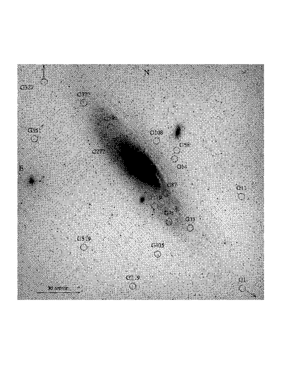
Figure 1: The positions of the observed fields overplotted on an image of M31.

In Fig. 1, the positions of the observed fields are overplotted on a $\sim 1\deg\times 1\deg$ image of M31, obtained using the Tautenburg Schmidt telescope. Our fields sample the disk and halo of M31 over a wide range of radii and positions, from $\sim$ 20 arcmin ($\sim$4.5 kpc) as far as $\sim$ 150 arcmin ($\sim$ 35 kpc) along the major and minor axes.

Table 1 gives the observed fields, which are designated by their associated globular cluster (using both Sargent et al. (1977) and Battistini et al. (1987) designations). The rectangular coordinates X and Y [arcmin] are reported in column 3 and 4, where the X axis coincides with the major axis of M31, and the Y axis coincides with the minor axis. $R=\sqrt{X^{2}+Y^{2}}$, the radial distance from the center of the galaxy, is reported in column 5, and the adopted reddening $E(B-V)$ is reported in column 6 (see sect. 2.2). Finally, we report in column 7 the approximate fraction of spheroid stars over the total ($F_{Sph}$), as estimated in sect. 2.1 (but see also Sect. 9,10 for discussion).

2.1 Expected contributions to the observed samples

Only the outermost lines of sight in M31 sample a pure halo population, and clear traces of a disk population are found even at those locations somewhat outside the faint disk isophotes. Therefore, we image some combination of disk and halo in most fields.

It is possible to derive an approximate estimate of the relative contribution of the disk and the spheroid along a particular direction using the models by Walterbos & Kennicutt (1988) which reproduce very well the surface brightness profiles of both components over a very wide range (see also Pritchet & van den Bergh, 1994). The fraction of light must scale as the fraction of light contributors (stars), at least to first order. Since the Walterbos & Kennicutt (1988) models refer to the major axis and minor axis profiles, reasonably good estimates can be obtained for the fields that lie in the vicinity of the axes.

The fields G33, G87, G287 and G322 can be considered to lie on the major axis. All of these fields are largely dominated by disk population. However, while G33, G322 and G287 are sufficiently far from the center and suffer only a marginal contamination by halo stars ($\sim 7$% for the first two fields and $\sim 12$ % for the latter), the growing importance of the bulge has some influence on the G87 field ($\sim 18$% of contribution by the spheroid).

The fields G76, G119 and G272 are clearly projected onto prominent features of the disk and their distance from the major axis is $<12^{\prime}$. Given their position with respect to the bulge, the contamination by spheroid stars can be assumed to be $<10$%. Obviously, the model of Walterbos & Kennicutt (1988) doesn’t include disk substructures such as spiral arms, and some fluctuation is possible. In particular the line of sight of G76 samples the $R=40^{\prime}$ring, the site of the most vigorous star formation in M31 (Hodge, 1992; Williams, 2002).

The fields G108, G64 and G58 are relatively close to the NW arm of the minor axis, so the contribution of the various components to their population mix can be more correctely estimated from the minor axis profile. The relative contributions of the spheroid are $\sim 60$ %, $\sim 65$ % and $\sim 70$ %, respectively. These lines of sight intersect the halo, but the contribution from the disk population is very important.

For the other fields a clearcut estimate based on the axis-oriented profiles cannot be done. However, all of them are farther than one degree from the center of M31 and most are expected to be dominated by the halo. In particular G319, not very far from the minor axis and at $Y=-68.9$ arcmin, can be considered a “pure halo” field; G11, G219 and G351 all have $Y>40^{\prime}$, and the contamination by disk stars is expected to be low ($<10$ %). G105 has $Y=-29.8^{\prime}$ and, judging from the minor axis profile the minimum contribution from the disk population should be $\sim 20$ %. Finally, G327 has $Y=5.1^{\prime}$ but is more than $2\deg$ from the center of the galaxy. The halo contribution as formally estimated from the major axis profile (with considerable uncertainty) is $\sim 6$ %, but the large distance from the center of the galaxy suggests that it may be considerably larger than this.

Contamination by foreground stars belonging to our own Galaxy and by background distant galaxies and quasars is also possible. This issue has been extensively discussed by Holland et al. (1996) who found the contamination from such sources on the final CMDs and luminosity functions to be negligible. We repeated their tests and confirm their results.

3 Observations and Data Reduction

The observational material is described in detail in Table 2, which gives: (1) the field identification, (2,3) right ascension and declination of the associated PC pointing, (4) date of the observations, (5,6) identification number of the $HST$ program that obtained the observations, and name of the program PI, and (7) filter and exposure time of the available CCD frames.

Most of the images are from the WF chips of exposures in which the PC was centered on the globular cluster (which was the prime target). One globular cluster, G327, was missed; our field is 36^′ from the cluster but we preserve our usual naming convention.

The G272 and G351 fields are parallel WFPC2 images from GO-5420, which imaged G280 and G351 using the FOC. Both fields are located at $<5^{\prime}$ of the respective clusters.

The G287 field was accidentally observed twice: G287b is slightly rotated relative to G287a. These data enable us to test our photometry (Sec. 3.4). Although we consider 17 fields, our survey actually has only 16 independent lines of sight.

The principal characteristic we want to stress here is the great homogeneity of the dataset. Of the 17 fields, 11 were imaged as part of the same proposal, and the integration times in each filter are identical. The other six image sets have been selected because of similar exposure times and choice of filters. Furthermore, all of the repeated exposures in each set were taken at fixed pointing and we verified that the relative position of each image within a data set coincides with the others to within a small fraction of a pixel. This allowed us to produce stacked images without any shift and/or interpolation (see below).

The distribution of stars within each field is very homogeneous over the scales sampled by the WFPC2 camera. Image crowding is an issue in all cases, with significant variations between the different fields, ranging from 640 resolved sources/sq. arcmin in the outermost halo fields, to 13000 resolved sources/sq. arcmin for those fields nearest the nucleus. Obtaining good photometry in such conditions is very difficult, since even the best PSF-fitting packages are subject to significant errors both in the photometry and in the interpretation of the detected sources. This class of problems are the most subtle and dangerous because they permit contamination by large numbers of spurious sources (e.g. see Jablonka et al., 1999). Since most of our fields are not lacking in sample size, we imposed quite severe selection criteria in order to clean our sample from spurious or badly measured sources. In some cases, up to 20% of the detected sources are rejected, under well defined and fully reproducible criteria which are described in the following subsections.

After several tests that allowed us to optimize all the parameters involved in any step of the data reduction process, we assembled a fully automated pipeline where the only input data are an estimate of the background level of the images, the exposure times and the dates of the observations. The pipeline carries out all the steps that are described in detail in the next subsections, from the PSF-fitting photometry on the stacked and cosmic ray cleaned images, to the production of the final calibrated and selected catalogue, every step being carefully checked.

The only key step requiring manual intervention is the determination of aperture corrections, where obvious bad measures or erroneous associations must be removed by hand (see sect. 3.2). Thus, also the data reduction process is strictly homogeneous for every image set. Its reproducibility has ben carefully tested by comparing the results obtained by different people reducing the same image set, and by the comparison of the results of the independent reduction of the two overlapping fields G287a and G287b. We stress the homogeneity of the data set and of the data analysis procedure because we believe that this is a fundamental issue for a systematic study, as the one presented in this paper.

3.1 Relative photometry

All the analysis was performed on the bias subtracted and flat field corrected frames from the STScI pipeline. The overscan region was trimmed and each set of repeated exposure images was coadded and simultaneously cleaned by cosmic ray spikes with the standard utilities in the IRAF/STSDAS package.

The PSF-fitting photometry was performed using the DoPHOT package (Schechter et al., 1993), running on two Compaq/Alpha stations at the Bologna Observatory. We adopted a version of the code with spatially variable PSF and modified by P. Montegriffo to read real images. A quadratic polynomial has been adopted to model the spatial variations of the PSF. The parameters controlling the PSF shape were set in the same way as Olsen et al. (1998), that successfully applied DoPhot to the analysis of WFPC2 images.

Inspection of the F814W images shows that they have a higher S/N in general than F555W despite their being exposed for equal times in most cases. This is not surprising given that most of the detected stars are old, metal rich RGB stars. A few preliminary tests convinced us to use the F814W frames for the source catalog, classifying as valid those sources brighter than 3 times the local background noise. We then forced the code to fit the same sources in the F555W images, using the so called “warmstart” option of DoPHOT.

Since DoPHOT provides a classification of the sources, we retained only the sources classified as stars (type 1, 3 and 7). We cross-correlated the F555W and F814W output catalogues with a tolerance of 1 pixel and finally produced a catalogue containing, for every image set, the positions in the frame, F555W and F814W instrumental magnitudes and the associated errors, as well as a parameter connected with the shape of the sources (ext = extendedness parameter, see Schechter et al., 1993). We found that in all cases the bulk of the sources classified as stars are confined in the range $-20.0\leq ext\leq 20.0$, and consequently we excluded from the catalogue all the outliers.

The CTE corrections have been applied according to Whitmore et al. (1999).

3.2 Calibrations

To transform the instrumental magnitude from the PSF-fitting photometry to the Johnson-Cousin and/or STMAG system it is necessary to apply the aperture corrections to a radius of $0.5$ arcsec, i.e 5 WF pixels (Holtzman et al., 1995).

Aperture photometry at a radius of 5 px was obtained for all the stars whose peak intensity was higher than ten times the local background noise and having no detected companion within a 15 px radius, using the Sextractor package (Bertin & Arnouts, 1996). Average aperture corrections were obtained for each field using these stars. Deriving reliable aperture corrections in such extreme (and uniform) crowding conditions is very difficult [see, for instance, Jablonka et al. (1999)]. Furthermore, because of the heavy undersampling of the PSF in the WF cameras, the flux sampled in the 5px aperture is strongly dependent on the exact position of the peak of the PSF within the central pixel of the star image (see Biretta, 1996). Thus there is no unique correction for all the stars but one has to rely on an average correction.

The total uncertainty in the absolute photometry introduced by the aperture corrections is in general $\pm 0.05$ mag, but can reach $\pm 0.11$ mag in the worst cases, a non negligible uncertainty indeed. However, these are the intrinsic and unavoidable limits of the WFPC2 as a photometer, at least in the presence of heavy, uniform crowding. It is interesting to observe that all the independently derived corrections are very similar (i.e. standard deviations are rather small), a fact that testifies the stability of the whole aperture corrections procedure. No trend of aperture corrections with position in the frame was detected to within the quoted uncertainties.

Once the aperture corrections were applied, the instrumental magnitudes have been reported to the Johnson-Cousin and STMAG systems using the standard calibration relations provided by Holtzman et al. (1995).

3.3 Cleaning from contamination

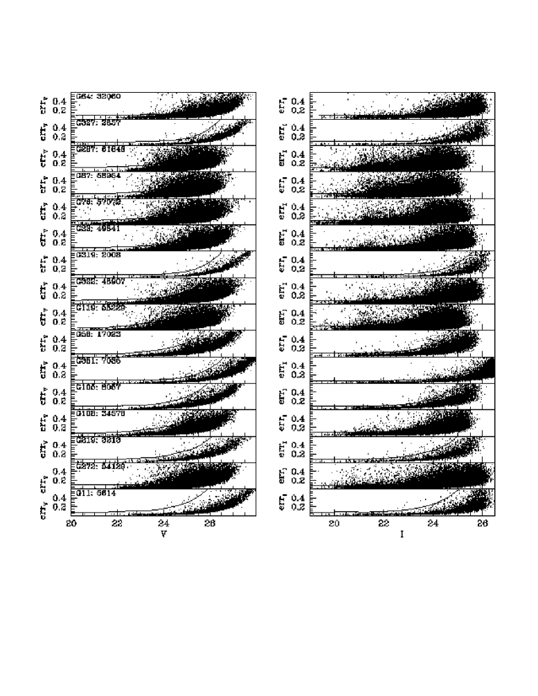
Figure 2: Photometric errors as a function of V and I magnitude. The lines represent the treshold for three times the average error. The points above the lines are excluded from the final sample.

In Fig. 2 the errors in the relative photometry for all the measured sources are shown as a function of magnitude. It can be readily appreciated that the mean uncertainties and the limiting magnitudes are determined primarily by the crowding conditions, and differences in exposure time are much less important. For all cases errors are smaller than $0.1$ mag for $V<24.5$. A check of the reliability of the errors provided by DoPHOT will be described in the next subsection.

All the stars with an associated error (either in V or in I magnitude) larger than three times the average error at their magnitude level were excluded from the sample, as well as all the stars having $err_{V}\geq 0.6$ mag and/or $err_{I}\geq 0.6$ mag. The average error as a function of magnitude was calculated applying a $2-\sigma$ clipping average algorithm on 0.5 mag wide boxes. The lines superimposed on the plots of Fig. 2 represent the $3\times err_{V}$ or $3\times err_{I}$ thresholds actually adopted. Errors much larger than the mean can originate from a number of reasons: bad interpretation by the PSF-fitting algorithm, exceptionally high and/or variable background, proximity to a very bright and/or heavily saturated source, proximity to chip defects, partial saturation, etc. In any case, our aim is to prevent contamination by spurious sources and this selection criteria is a very effective one.

A careful comparison between the derived catalogues and the corresponding images showed us that there were still three categories of undesirable sources that passed all the selection criteria applied, i.e.:

1. Spurious stars detected in diffraction spikes and coronae around heavily saturated stars (type a).

2. Faint spurious stars detected in luminous extended background galaxies (type b).

3. Faint background galaxies misinterpreted by the code as stars (type c).

Identification and hand removal of the type a and b sources was completed for all the fields with $n_{source}\leq 35000$ stars (see Fig. 2). In the same fields some type c sources have been indentified by accurate visual inspection of the frames, but some faint galaxies probably remain in the final catalogues. For the remaining fields ($n_{source}\geq 48000$) the crowding prevented any further cleaning. However the spurious sources represent a negligible fraction of the samples: 3545 sources of type a,b and c were removed over a total of more than 100000 in the inspected fields ($<3.5$ %).

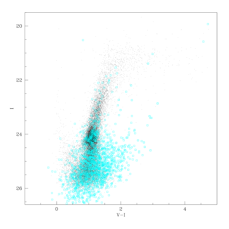
Figure 3: The manually removed contaminating sources (open squares) from the entire sample superposed on the Color Magnitude Diagram of the field G64. Most of the sources redder than $(V-I)\sim 1.5$ are galaxies or spurious stars from the decomposition of extended galaxies, most of the sources bluer than this figure are spurious stars from spikes and/or coronae of heavily saturated stars

Fig. 3 shows the rejected sources superposed on the CMD of the G64 field. Most of them are type a sources that lie upon the real stars distribution, mainly populating the region $(V-I)\leq 1.5$, while sources of type b and c are redder than this value. The blue region of the diagram is little affected by this kind of contamination. If the faintest objects are excluded (those with $I\geq 26$), only $10$ % of the spurious sources populate the $(V-I)<0.8$, $65$ % are found in the range $0.8\leq(V-I)\geq 1.5$ and $25$ % are redder than $(V-I)=1.5$. Most of the spurious sources are rather faint, $58$ % of them lie below the red HB clump ($I<24.5$), while the upper RGB is nearly free of contamination, only $8$ % of spurious sources being brighter than $I=23.5$.

We can safely conclude that any spurious sources possibly surviving these cuts could not affect the interpretation of our CMDs, that are largely dominated by bona fide stars; in particular, the RGB and red HB that we consider in this study are clean.

3.4 Reproducibility of measures and reliability of errors: a direct test.

The large overlapping area of the G287a and G287b fields made it possible to perform a direct test of the reliability and reproducibility of our measures. As this is the most crowded field of the whole set, it assures that we are testing the entire procedure under the most unfavorable conditions. Thus the uncertainties derived from this comparison are conservative.

Both images were independently reduced, from the raw frames to the calibrated and selected catalogue, including aperture corrections. The comparison was finally performed for each WF chip separately. First, it has to be noted that virtually all the stars in the overlapping areas were measured in both image sets and independently survived the selections. Thus the detection and selection criteria are very stable and reliable.

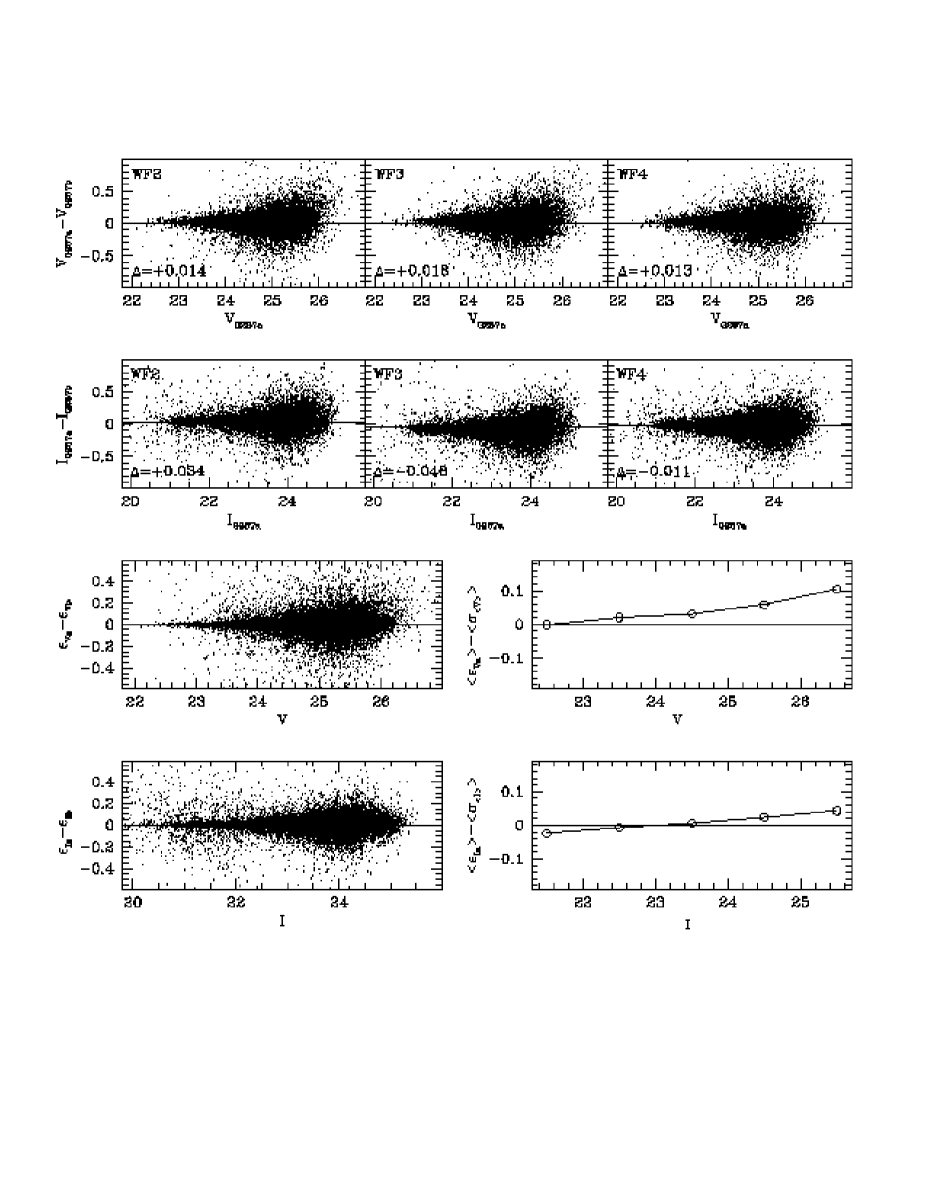
Figure 4: Comparison between the photometry of the stars in common in the fields G287a and G287b. In the upper two panels the difference in the final calibrated magnitudes is shown for the three WF cameras independently (first panel: V magnitudes, second panel: I magnitudes). In the lower two panels are reported the differences between the errors as computed by DoPHOT and the error on the mean obtained by the two repeated measures of the stars in common, versus magnitude in the corresponding filter (third panel: V, fourth panel I. The differences has been averaged over 0.5 mag boxes. The errors provided by DoPHOT are good estimates of the true photometric uncertainties.

In the upper two panels of Fig. 4 the magnitude differences as a function of the G287a magnitudes are shown, for all the stars in common. Note that in 4 out of 6 cases, the absolute average differences are $<0.02$ mag and in all cases they are $<0.05$ mag. This demonstrates that the uncertainties in the field-to-field relative photometry are fairly small in the final calibrated catalogue, i.e. the whole sample of 17 data sets is tied to a common photometric system that is homogeneous to $<0.05$ mag. The reproducibility of the results is excellent.

Individual uncertainties in the relative photometry are nearly as important as the measurements themselves. DoPHOT, as well as many other popular photometry packages, derives the errors in each measurement mainly from the signal to noise ratio of the fitted images and from the errors in the fitting procedure. While the approach is formally correct and usually produces a correct ranking of the quality of the measures, it is not guaranteed that the absolute estimate of the error is correct. The ideal estimate should be derived from the dispersion of many repeated measures, a procedure clearly not viable in the present case. In the lower panels of Fig. 4 the differences between the errors from DoPHOT ($\epsilon_{Va}$, $\epsilon_{Ia}$) and the error on the mean from the two measures obtained for the stars in common ($\sigma_{<V>}$, $\sigma_{<I>}$) are averaged over 1 mag intervals and plotted versus V and I magnitudes. The two quantities are well correlated and their difference is generally lower than 0.03 mag. Furthermore, DoPHOT seems to slightly overestimate errors, thus the most dangerous occurrence is prevented, i.e. drawing conclusions that are not supported by the true intrinsic accuracy of the data.

4 The Color Magnitude Diagrams

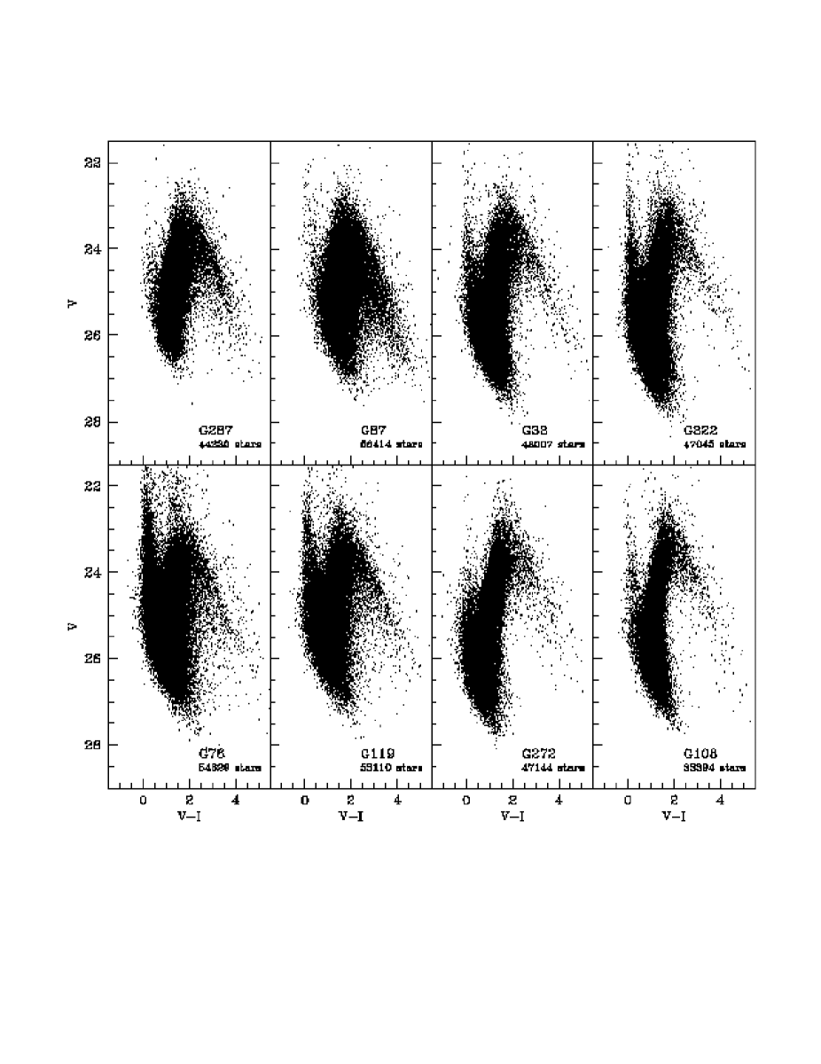
Figure 5: The (V,V-I) Color Magnitude Diagrams for the fields: G287, G87, G33, G322, G76, G119, G272, G108. In this figure and in figure 6 the diagrams are shown in order of increasing distance from the major axis, with the only exception of G327 (see text).

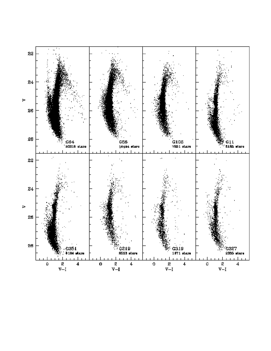
Figure 6: The (V,V-I) Color Magnitude Diagrams for the fields: G64, G58, G105, G11, G351, G219, G319, G327. See the caption of Fig. 5.

Final CMDs for all of the 16 fields are shown in Figures 5 and 6. The diagrams are ordered (from top to bottom and from left to right) according to the projected distance of the field from the major axis X (see Fig.1). The only exception is the field G327 that is the outermost one (130  arcmin from the center of the galaxy) but is relatively close to the major axis and has been plotted as last. Note that nearly the same order is obtained ranking the CMDs by increasing contribution from spheroid stars, as reported in column 7 of Table 1.

The limiting magnitude depends mainly on crowding. The deepest photometry reaches $I\sim 27$ (G351) but on average is about $I\sim 26$. Stars brighter than $I\sim 20.5$ are partially saturated. Despite the large differences in positions among the fields, the diagrams are quite similar if one takes into account the differences in the number of sampled stars.

4.1 The main morphological features

Our color-magnitude diagrams display the following common features:

• A red and broad RGB, ranging from $(V-I)\approx 1$ to $(V-I)\approx 4$, with the RGB tip near $I\approx 21$, and a prominent red clump (RC) on the RGB and HB, at $(V-I)\approx 1$ and $I\approx 24.3$. In all fields the upper part of the RGB bends towards redder colors and fainter magnitudes in the $V$ vs $(V-I)$ CMD, a characteristic seen in metal rich globular clusters and caused by TiO blanketing in metal rich first ascent stars. These characteristics are consistent with a relatively high metallicity and a wide abundance range.

  The presence of the dominant red clump in all of the halo fields is prima facie evidence for an old metal-rich stellar population in the halo, which is most likely a mixture of intermediate age RGB stars over the full metallicity range and metal-rich old halo HB and RGB stars. The high metallicity is also consistent with the slope of the RGB.

• A blue plume at $(V-I)<0.5$, reaching in some cases $I\sim 20$, is very evident in some of the CMDs. This feature can be identified with the main sequence of an intermediate/young population (YMS).

  Despite the large number of sampled stars, the YMS is barely noticeable in the G287 and G87 fields, while it is clearly present in G33, G322, G119, G272, G108 and G64, and it is strongly present in the G76 field.

  The existence of a sparse YMS cannot be excluded in the fields G58, G11 and G351. In the last two cases the low total number of stars in the sample prevents any firm conclusion in this sense. In any case, the good anti-correlation between the prominence of the YMS and the estimated $F_{Sph}$ is remarkable.

• A small number of blue HB stars at $(V-I)\sim 0.5$ and $I\sim 24.5$ is present in many of the halo fields (e.g. G11, G105, G219, G327, G319, G319 and G351), and could be also present, but hidden within the YMS population, in the other fields (see e.g. G64).

  These stars indicate the presence of some globular-cluster age metal poor stars, because presumably only stars older than 12 Gyr can reach the blue HB. Their numbers ($\approx 15$% of the RHB) are consistent with the fraction of metal poor stars in the abundance distributions that we derive from the RGB.

• In the CMDs where the YMS is most conspicuous, a red plume is seen between $I\sim 22$ and $I\sim 20$, around $(V-I)\sim 1.5$. Because of the strong young stellar population, we interpret stars in this region as being red supergiants, the evolved counterpart of the YMS stars.

We represent the CMD of the G76 field as a contour plot (Hess diagram) in Fig. 7, in order to illustrate more clearly the principal features present in all of our fields.

The most prominent feature common to all of the CMDs (other than the red giant branch) is the Red Clump, which shows an elongated structure with a very sharp peak. The few stars brighter than $I\sim 21$, beyond the RGB tip, could either be cool RSG and/or bright AGB stars, the latter not necessarily indicative of the presence of intermediate age populations, [see Guarnieri et al. (1997)]. There is also a real possibility that some of these are simple blends of normal RGB stars, since this is expected in extremely crowded fields [see Jablonka et al. (1999), in particular their figs. 5a and 5d, and see also Renzini (1998)].

An accurate treatment of the blends, requiring a large number of artificial star experiments, is important for some issues (e.g. to constrain the fraction of intermediate-age stars in the halo) that are beyond the scope of the present paper.

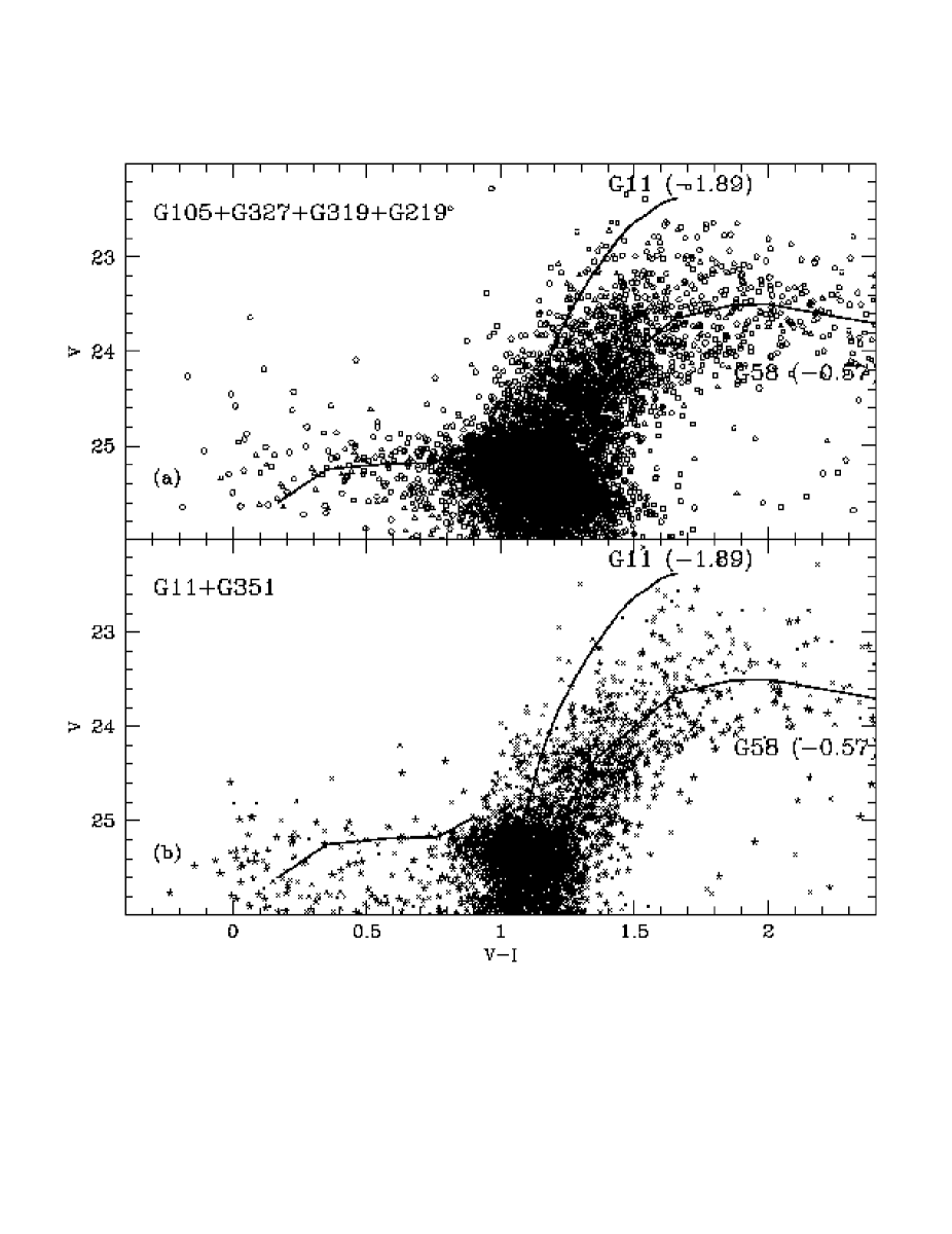
Figure 8: CMD for the coadded halo fields zoomed to show the details of the HB morphology (see text). The lines superimposed to the plot are the HB fiducial for M68, shifted by $\Delta$V=9.44 and $\Delta$V-I=0.09 to match the blue HB of the M31 fields, and the RGB ridge lines of the M31 globular clusters G11 ([Fe/H] = -1.89) and G58 ([Fe/H] = -0.57). Panel (a) the CMDs of G105, G327, G319 and G219. Stars from different fields are marked with different symbols (G105: pentagons; G327: circles; G319: triangles; G219: squares). Panel (b) the CMDs of G11 and G351 (G11: $\times$s; G351: stars). The BHB of the CMDs presented in panel (b) is contaminated by an apparent blue plume that is not present in the CMDs of panel (a).

Figure 8$a$ shows stars from the halo fields G105,G219, G319 and G327 are plotted together in the same (V,V-I) CMD, centered on the Horizontal Branch. To limit the contamination from spurious measures, we plot only the stars with photometric errors less than 0.15 mag in both passbands.

The BHB is clearly visible at $V\sim 25.2$, extending from the red HB clump to $(V-I)\sim 0$, as previously found by Holland et al. (1996). A schematic ridge line derived from the HB of the metal poor globular cluster M68 [data from Walker (1994)] is superimposed on the plot, applying a shift of 9.44 mag in V and 0.09 mag shift in color.

Fig. 8$b$ shows the CMDs of the fields G11 and G351, plotted as in panel (a). A BHB similar to that shown in panel (a) is still present, but in this case the feature is partially contaminated by fainter stars looking like the base of the YMS blue plume described above, and this is the reason why the CMDs are plotted separately. Considering the distance of G11 and G351 from the disk, the blue stars might also be field blue stragglers.

As G11 and G351 are among our deepest fields, we cannot exclude such a blue plume from the other fields either. Given the complexity of the M31 halo, it is possible that intermediate-age populations are distributed throughout the halo in various tidal streamers, present in some fields and not (or less) in others. The only secure determination of the nature of these faint blue stars will be imaging deep enough to reach the old main sequence turnoff at $M_{V}=+5$. However, even from the present data sets we can already deduce that subtle and possibly important differences may exist in the stellar populations of the outer fields of the M31 halo.

4.2 The intermediate-young population

In those fields with a substantial disk contribution, the presence of a blue plume is evidence of star formation within the last 0.5 Gyr. The power of our survey is that we can use deep imaging over a range of fields, enabling us to probe well past the few Myr of star formation history revealed by the brightest OB stars and HII regions.

Any attempt to derive the star formation history (SFH) from the CMDs and LFs would need a detailed analysis based on the comparison with appropriate synthetic evolutionary tracks and taking into account all the observational effects [see, e.g. Tosi et al. (1989), and Aloisi et al. (1999); Gallart et al. (1999); Hernandez et al. (1999) as examples of recent applications]. Williams (2002) performed a similar type of analysis in M31 using 27 fields imaged by $HST$ along the disk, in order to determine the star formation history that best fits his observations.

This type of detailed study is beyond the scope of the present paper; however, it is possible to apply a simple analysis to our data and obtain useful information to constrain the relevant timescales and stellar masses associated with the prominent YMS of many disk-dominated fields. This aim can be easily achieved by comparison with theoretical isochrones, and would also help to set a basic interpretative scheme for the CMDs we present.

In order to compare our CMDs to theoretical quantities, however, we need to make assumptions on two basic parameters, reddening and distance modulus.

• $Reddening-$ Interstellar extintion toward M31 can be due to dust screens residing either in our Galaxy or internal to M31 itself. While a reliable estimate of the average reddening due to the Milky Way can be obtained from reddening maps (Burstein & Heiles, 1982), estimates of the “intrinsic” reddening are not available and this is one of the major sources of uncertainty in the study of stellar populations in M31 [see the thorough discussion by Barmby et al. (2000)]. These latter authors attempted to estimate the total reddening toward the M31 globulars, calibrating the relations between integrated colors (essentially B-V) and metallicity with Galactic globulars for which the amount of reddening is known from independent measures.

  We have applied a similar relationship to the integrated colors and metallicities of the globular clusters associated with the fields that are projected onto clear disk structures, i.e. that are more likely affected by intrinsic extinction. For G76, G87, G119, G272 and G287 we find an average $<E(B-V)>=0.14$ and $\sigma_{E(B-V)}=0.03$. We decided to adopt this value since the single values were remarkably similar and to avoid the introduction of noise due to the uncertainties of the calibration.

  For all the remaining fields that are distant from the high surface brightness regions of the disk we adopt the Galactic reddening toward M31. Following Hodge (1992), we adopt $E(B-V)=0.11\pm 0.02$ from McClure & Racine (1969); we use the Dean, Warren & Cousins (1978) extinction law $E(V-I)=1.34E(B-V)$ and $A_{I}=1.31E(V-I)$.

• $Distance-$ We adopt the Cepheid distance modulus of $(m-M)_{0}=24.43\pm 0.06$ ($\sim 770$ kpc) from Freedman & Madore (1990). Other distance estimates may be found in Table 3.1 in van den Bergh (2000).

4.2.1 The age range of the YMS stars

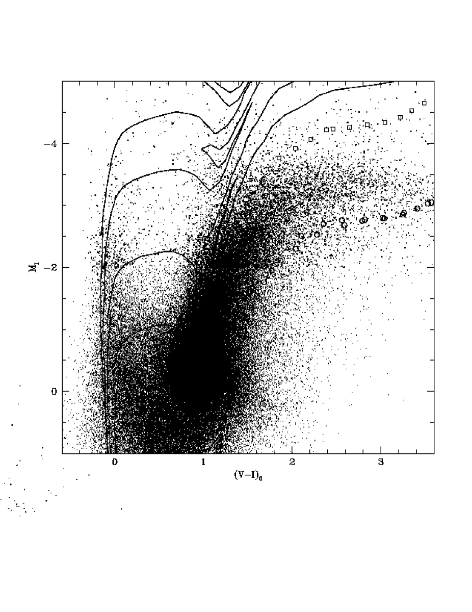
Figure 9: CMD of all the 154784 stars from the disk-dominated fields G76, G119 and G322, reported to the absolute plane $[M_{I},(V-I)_{0}]$. Isochrones at $[Fe/H]=0.0$ and $Y=0.28$, from the set of Bertelli et al. (1994) are superimposed on the diagram. The continuous lines are isochrones of age t = 60, 100, 200 and 400 Myr, from top to bottom. Open squares and circles correspond to isochrones of t = 1 and 12 Gyr, respectively. The stars brighter and fainter than the $M_{I}=-2$ threshold are shown as points of different thickness to allow easier recognition of both the densely populated features in the lower part of the CMD (e.g. the HB Clump) and the sparse bright features (e.g. the upper MS and the red plume of RSG stars

Fig. 9 shows the CMD (in $M_{I},(V-I)_{0}$ for the sum of the disk-dominated fields G76, G119, and G322 (154,748 stars). The stars above and below the $M_{I}=-2$ threshold are plotted using points of different thickness to allow easier recognition of both the densely populated features in the lower part of the CMD (e.g. the HB clump) and the sparse bright features (e.g the upper MS and the red plume of RSG stars).

Six isochrones with solar metallicity and helium abundance $Y=0.28$, from the set by Bertelli et al. (1994), are superimposed to the diagrams. They correspond to ages of 60, 100, 200 and 400 Myr (from top to bottom, continuous lines), 1 Gyr (open squares) and 12 Gyr (open circles). Our adopted composition seems the most appropriate for intermediate/young populations in the disk of a large spiral galaxy.

Before we consider Fig. 9, recall that the brightest MS stars known in M31 reach $M_{V}\sim-6.2$, but the saturation level in our survey occurs at $M_{V}\sim-4$, which eliminates the brightest main sequence stars from our sample.

The isochrones of 60, 100, 200 and 400 Myr fit well the observed distribution of young and intermediate age stars, thus constraining the age range associated with the sampled YMS.

The RSG branches of these isochrones group between $(V-I)_{0}\sim 1$ and $(V-I)_{0}\sim 1.6$, providing an excellent fit to the red plume described in the previous section (figures 6 and 9). The 1 Gyr isochrone illustrates clearly how intermediate age AGB stars can populate the region of the CMD immediately above the RGB Tip.

As a final consideration we note that RGB stars as red as (or redder than) the 12 Gyr isochrone are clearly present in the composite CMD of Fig. 9. The obvious conclusion is that very old and very metal rich stars are found in the disk of M31.

4.2.2 A Classification Scheme for the Blue Plume Population

In order to model the main sequence luminosity function we have grouped stars by luminosity bins so that they crudely sample different mass ranges. We can use these counts to explore the relative importance of the YMS in different fields.

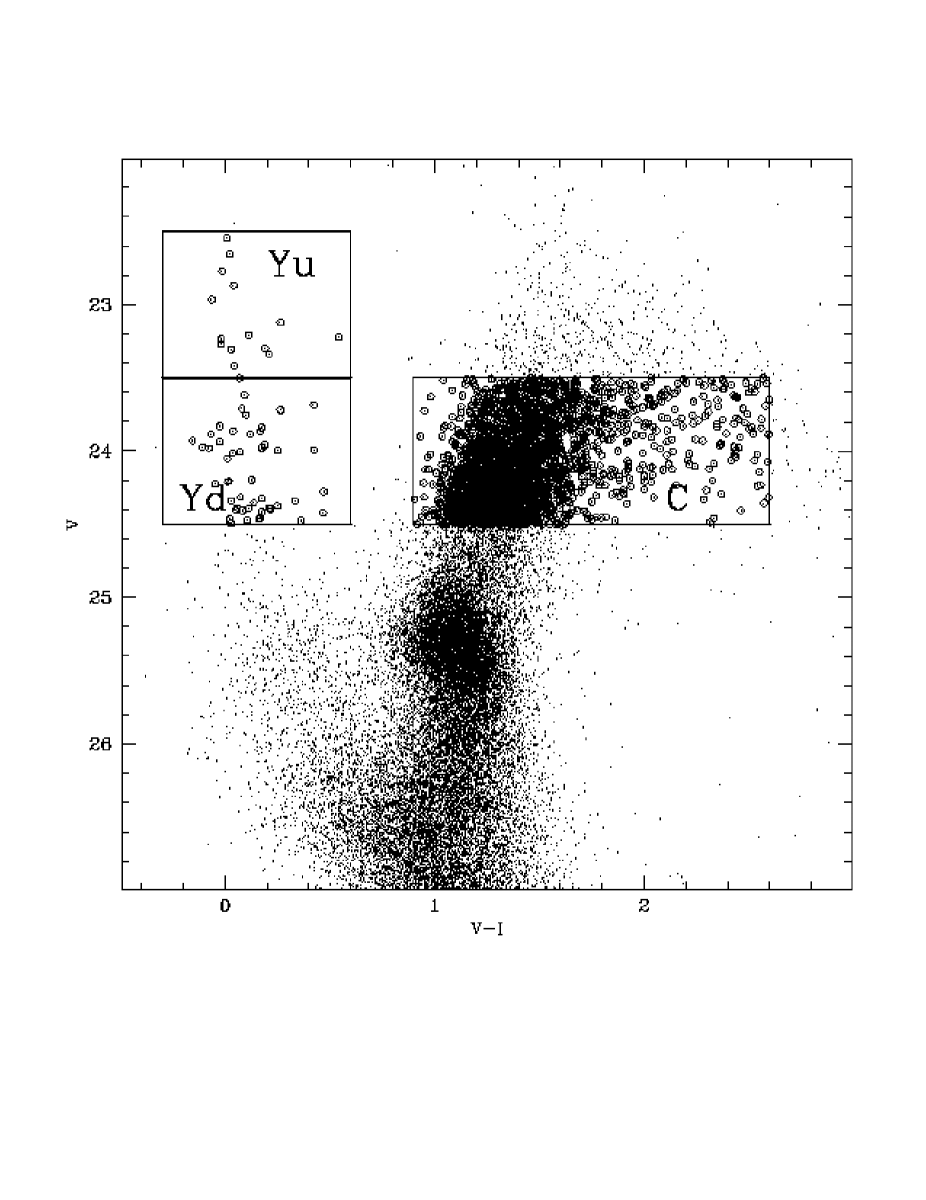
Figure 10: The population boxes defined to study the YMS are evidenced in the [V,(V-I)] CMD of the G64 field. The boxes marked with Yu and Yd samples different part of the Main Sequence, while the box marked with C has been defined for normalization purposes. The stars falling into the indicated boxes has been indicated with open circles.

In Fig. 10 we overplot 3 boxes on the (V,V-I) CMDs of the G64 field, as an example. These boxes are rather large and clearly separated in order to include a portion of a particular sequence independent of any slight difference in reddening or metallicity among the different fields.

The regions are defined as follows:

1. Yu: ($23.5<V\leq 22.5$ and $-0.3\leq V-I\leq 0.6$) samples the upper YMS. The number of stars in this part of the CMDs are indicated as $N_{Yu}$.

2. Yd: ($24.5<V\leq 23.5$ and $-0.3\leq V-I\leq 0.6$) samples the lower YMS. The number of stars in this box are indicated as $N_{Yd}$.

3. C: ($24.5<V\leq 23.5$ and $0.9\leq V-I\leq 2.6$) samples the RGB in the same magnitude range as Yd. The number of stars in this box are indicated as $N_{C}$. We will use $N_{C}$ to normalize the star counts in the previous boxes.

According to the same set of isochrones shown in Fig. 9 it can be stated that the Yd box samples stars younger than $\sim 0.5$ Gyr while the Yu boundary samples stars younger than $\sim 250$ Myr. We thus derive the following indices::

• $(N_{Yu}+N_{Yd})/N_{C}$: ranks the fields according to the relative importance of the YMS population.

• $(N_{Yu}/N_{Yd})$: since more massive (i.e. younger) YMS stars are expected to reach brighter magnitudes, this ratio tests differences in the recent star formation history between the different fields.

The errors in the star counts have been estimated according to Poisson statistics, and we propagate the errors to derive errors in the indices. It is obvious that our detection of the bright MS is most significant for the most populous, disk dominated fields. The fields G11, G58, G105, G219, G319, G327 and G351 have too few young stars to be worthy of further consideration in this sense. As already noted, this doesn’t necessarily mean that no young stars are present in these fields, since the low total stellar density can prevent the detection of short lived stars. However, a comparison with the most similar field having a significant YMS population, i.e. G64, shows that these fields are intrinsically deficient of “Yu+Yd” stars by a factor $\sim 2-5$ with respect to G64.

Fig. 11 shows $(N_{Yu}+N_{Yd})/N_{C}$ (panel a) and $(N_{Yu}/N_{Yd})$ (panel b) plotted as a function of the distance from the center of the galaxy, deprojected to “face-on” $Rp_{[arcmin]}$ (see Hodge, 1992, and references therein). The deprojection has been obtained adopting $i=12.5\deg$, and it is justified in the present case since we are dealing with $(i)$ mostly disk dominated fields in the plane of M31, and $(ii)$ the YMS population which is expected to be located in the star forming disk.

The prominent feature appearing in panel (a) is the strong peak in the relative abundance of stars younger than $\sim 0.5$ Gyr occurring at $Rp\sim 60^{\prime}$, shown mostly by G76 but also by G119 and G322. This corresponds to the $R\sim 10$ kpc ring in which neutral hydrogen and virtually any tracer of a young population seem to cluster (Hodge, 1992; van den Bergh, 2000). This main structure of the star forming disk is clearly sampled by our fields as a very significant enhancement in the recent star formation rate: there is a factor $\sim 35$ in the relative abundance of YMS stars between the nearly quiescent inner regions (fields G87, G287) and the peak of the ring structure (field G76).

In panel (c) of Fig. 11, we show the $(N_{Yu}+N_{Yd})/N_{C}$ index as a function of the absolute distance along the major axis ($|X|$), to provide a different view of the results presented in panel (a).

In particular, this panel allows a direct comparison with the distribution of disk tracers as depicted by Hodge (1979) (see his Fig. 7 and 8). The agreement is indeed remarkable, and the general picture assembled by Hodge (1992) is confirmed by our survey, at least to the extent permitted by our limited spatial sampling.

Panel (b) shows that also the star formation in the last 250 Myr was particularly strong near the position of the G76 field. However, the most noteworthy feature is the high $N_{Yu}/N_{Yd}$ value in the innermost field G87, indicating that most of the (weak) star formation in this field occurred quite recently.

This is particularly interesting in comparison with the otherwise similar field G287 that shows a $N_{Yu}/N_{Yd}$ a factor $\sim 5$ lower for the same value of $(N_{Yu}+N_{Yd})/N_{C}$.

As a result of these considerations, we can conclude that the star formation rate has varied significantly over the last 0.5 Gyr in different regions of the disk of M31. Although our findings are not based on as sophisticated an analysis as that of Williams (2002) we agree with the conclusions of that study. It is noteworthy that the observable activity in the 10 kpc ring corresponds to recent significant star formation, and that recent star formation activity is not necessarily correlated with a high total rate of star formation. Surveys with the $HST-ACS$ and more sophisticated modelling will greatly improve our understanding of this issue.

5 Assumptions and procedures for metallicity determinations

It is well known that the color of the RGB of an old Simple Stellar Population [SSP, i.e. an ensemble of stars sharing the same age and chemical composition, see Renzini & Buzzoni (1986)] is mainly affected by the abundance of heavy elements and only at a lesser extent by the age of the population. The influence of age becomes smaller and smaller with increasing age and it is almost negligible for ages in excess of $\sim 10$ Gyr. In principle, the metallicity of a RGB star is uniquely determined by its color and luminosity, once its age is known and a suitable calibration is available. The obvious application of such principle is to derive the metallicity distribution for a given population from the distribution in color and magnitude of its RGB stars (see Saviane et al., 2000).

However, when dealing with a Composite Population (CP), i.e. a mix of stars of different ages and metallicities, there are two main factors that can affect the correct recovery of the underlying metallicity distribution:

• AGB sequences, in general, run nearly parallel to the RGB but are slightly bluer. In the absence of any useful criterion to exclude them from the sample, they would appear as more metal deficient than their parent population, introducing a bias in the metallicity distribution (see Holland et al., 1996).

  The existence of a blue HB (as well as the results of the spectroscopic survey by Guhathakurta et al., 2000) tells us that a metal poor old population exists for sure. Hence, the blue side of the RGB must contain their metal poor giant precursors. If this is the case, contamination from AGB stars is necessarily very small since their lifetimes are significantly shorter than lifetimes on the RGB. In fact, for a solar metallicity population of age 15 Gyr, the number of RGB stars is predicted to overwhelm the number of AGB stars by a factor $\sim$ 40 (Renzini, 1998). Based on the above considerations, only a very small fraction of our metal poor giants may, in principle, be misclassified AGB stars.

• Age differences at fixed metallicity produce a widening of the RGB that could be erroneously interpretated as a metallicity range. This effect is rather subtle, since it depends on the whole star formation and metal enrichment histories of the composite population under study.

  For example the RGB of an old population (say $\sim 12$ Gyr) of solar metallicity can be contaminated by stars from a population of the same metal content but several Gyr younger that would simulate the presence of older metal poor stars [see sec. 3.6.1 of van den Bergh (2000)].

  The metallicity distributions (MDs) derived from the color distributions of RGBs in our CMDs are based on the assumption that the observed RGBs are dominated by old stars.

  This hypothesis is not at odds with observational evidence [see Tinsley & Spinrad (1971); van den Bergh (2000); Hodge (1992), and references therein], and all the numerous attempts made in previous studies are based on it (Rich et al., 1996; Holland et al., 1996; Pritchet & van den Bergh, 1994; Richer et al., 1990; Morris et al., 1994; Jablonka et al., 1999, 2000; Durrell et al., 1994; Couture et al., 1995; Durrell et al., 2001; Ferguson & Johnson, 2001; Harris & Harris, 2000, 2002; Sarajedini & Van Duyne, 2001).

  However, our previously stated caveats should be kept in mind when drawing any conclusion from the derived abundance distributions. This is especially true for the abundance distributions measured in those fields dominated by disk stars.

In addition to the above issues related to a composite population, there is a third problem one must take into account, i.e. the differential reddening that might affect the photometric data especially in the disk dominated fields.

Differential reddening does not seem to affect significantly any of our fields at a cursory inspection: for example, the wide RGB is found in distant halo fields, and no dispersion of the red clump along the reddening vector is seen in any field. Further, the blue main sequence, where present, is not similarly broadened.

However, we tested possible variations in interstellar/intergalactic extinction across the observed fields by comparing the CMDs obtained from different subsections of each single WFPC2 field. In every case we failed to detect any difference in the location of the main branches, and we conclude that variations of the extinction across the observed fields, if any, are negligible with respect to the intrinsic width of the branches and the observational errors.

Variations of the extinction along the line of sight could also affect the CMDs, but this effect would be more subtle. Dust structures in M31 might be embedded in the population, with some stars in front and some behind the cloud. However, the striking similarity between MDs (see Sect. 6.2) of fields sampling dense and active regions of the disk (f.i. G287, G33, G76) and those sampling outer halo lines of sight (f.i. G319, G351, G1), that are expected to be unaffected by M31 dust, argues against this type of differential extinction. To obtain such a result from a dataset where differential reddening has a significant effect in some fields and none in others would imply an implausible fine tuning between differential reddening, metallicity distribution and star formation history.

We conclude that differential reddening has at most a marginal effect on our CMDs and MDs.

5.1 The grid of Galactic Globular Cluster Templates

In our analysis we shall adopt as a reference system the Carretta & Gratton (1997) (CG) abundance scale, that is tied to high-resolution spectroscopy and offers a better guarantee of accuracy and reliability with respect to the Zinn & West (1984) (ZW) metallicity scale, that was based on photometric indices. However, the ZW scale has been and still is widely used, so we shall comment our results by comparing the effects of both scales (see Sect. 7.1).

For a detailed description of the CG vs. ZW scales we refer to Carretta & Gratton (1997). Here we just note that the CG scale yields more metal-rich values in the interval $-2<[Fe/H]<-1$ (this effect disappearing progressively as one moves towards the edges of this interval) and more metal-poor outside. Also, the metal-rich extension towards solar values is still poorly sampled and very uncertain for both scales, with CG yielding slightly more metal-poor values than ZW.

As we will discuss below, the choice of the CG or ZW metallicity scale has little effect on our main conclusions concerning the overall properties of the derived MDs. In fact, the same general conclusions can be drawn by a direct comparison of the star color distributions with the grid of the RGB ridge lines for Galactic GCs of known metallicity. However, the detailed shape of our abundance distributions and, therefore, some specific conclusions may indeed be affected by this choice (and, more significantly, by the adopted globular cluster grid and interpolating procedures).

Finally, we caution the reader that systematic effects on the zero-points of magnitudes and colors or of the metallicity scales may actually have the strongest impact on the overall picture.

For the metallicity determinations we adopt an approach similar to Holland et al. (1996), i.e. we compare the observed RGBs with a grid of accurately chosen RGB fiducial ridge lines at various metallicities, and then derive a metallicity estimate for each star by interpolating from the grid of templates. We apply the technique in the $[M_{I},(V-I)_{0}]$ plane since in this plane the behaviour of the RGB sequence is less susceptible of “curvature” effects (see Saviane et al., 2000).

As RGB templates we adopt the ridge lines of the galactic globular clusters NGC 6341 ($\rm[Fe/H]_{CG}=-2.16$), NGC 6205 ($\rm[Fe/H]_{CG}=-1.39$), NGC 5904 ($\rm[Fe/H]_{CG}=-1.11$) and 47 Tuc ($\rm[Fe/H]_{CG}=-0.71$) from Saviane et al. (2000).

As noted by all the authors adopting the present approach, the extension of the grid to more metal-rich values than 47 Tuc is quite difficult (for the lack of suitable candidates) and extremely uncertain (for intrinsic uncertainties in the high-Z regime).

After a careful revision of the available data, we choose to adopt for the very metal-rich regime two clusters, NGC 6553 and NGC 6528, for which sufficiently good V,I data and metallicity estimates (for both CG and ZW scales) are available.

Therefore we completed the reference grid with the ridge line of:

NGC 6553 ($\rm[Fe/H]_{CG}=-0.16$, Cohen et al. (1999)) obtained from the photometric data of Guarnieri et al. (1997), and

NGC 6528 ($\rm[Fe/H]_{CG}=+0.07$, Carretta et al. (2002)) obtained from the photometric data of Ortolani et al. (1995).

Reddenings and distance moduli are taken from the compilation by Ferraro et al. (1999), since their approach in the measure of distance moduli is homogeneous for all the clusters and independent of their HB morphology or of the presence of RR Lyrae variables. Table 3 includes these values and the metallicities of our calibrating clusters.

Before proceeding further, we wish to add a few considerations on the problems and implications the choice of a different grid may have on the subsequent analysis.

All previous studies dealing with a similar procedure of deriving the MDs from the color distributions of the giant branches in the CMDs have adopted their own custom-tailored recipe and reference grid (see Sect. 8). Some authors have adopted purely empirical grids or, alternatively, purely theoretical ones, others have adopted a mixture of both, using GC data to set the zero-point of a given set of theoretical models, or adding suitably calibrated isochrones to empirical templates to cover missing parts of the metallicity range. Furthermore, within each adopted procedure, the choice of selected GCs and/or set of models differs from study to study. Though the bulk of the main results is probably independent of these differences, there is no doubt that the detailed shapes and properties of the MDs are strongly affected and, especially in the very high-metallicity regime, these choices may dominate the results.

The reader should be aware that the same original data, transformed into MDs with different recipes, may yield significantly different results in some details. Coupled with the intrinsic, quite high uncertainties still affecting the observational data-bases themselves, one has to admit that all our analyses are still at a rather preliminary stage and far from offering an unambiguous detailed comprehension of this issue (see Harris & Harris, 2002, for discussion).

We have emphasized above that our reference grid relies only on empirical templates, chosen to be a homogeneous and reliable set, and sufficiently sampled to cover the relevant metallicity range in suitably fine steps. The accuracy of this approach depends only on observable quantities, i.e. photometric and spectroscopic data and reddening estimates, whose errors can be known and minimized to some extent, within the present possibilities. The use of theoretical models, that would be in principle easier and more precise, suffers of its own set of problems. In fact, while great progress has been made in producing synthetic RGB sequences, the physics of late-type stellar atmospheres (e.g. convection, alpha enhancement, etc.) and the color-temperature calibration, bolometric corrections, etc. are still poorly known, and the use of theoretical RGBs might introduce additional uncertainties which are difficult to correctly estimate and quantify.

5.2 The procedure of metallicity determination

Both the M31 CMDs and the templates are transformed to the absolute plane, using the values of reddening and distance quoted in Sect. 4.2 for M31, and listed in Table 4 for the templates.

The estimates of metallicity are performed on stars having $-3.9<M_{I}<-2.0$ and $0.90<(V-I)_{0}<4.0$. The reasons of this choice can be summarized as follows:

• Lower Luminosity limit: $M_{I}<-2.0$

  to retain the region of the RGB with the highest sensitivity to metallicity variations and to avoid contamination by RC stars. This choice also avoids the inclusion in the sample of the AGB clump stars, which are predicted (and observed) to lie around $-1<M_{I}<-1.6$ (see Ferraro et al., 1999). Thus the more densely populated feature of the AGB is excluded and we can be confident that only a marginal fraction of old AGB stars may contaminate our metallicity distributions.

• Upper Luminosity limit: $M_{I}>-3.9$

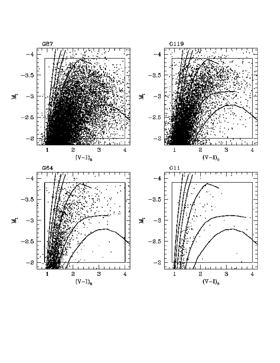
Figure 12: CMDs of the upper RGB in the absolute plane, for four fields, illustrating the full range of crowding in the data set. The ridge lines of template galactic globular clusters are superimposed to each plot. From left to right (CG metallicity scale): NGC 6341 ($\rm[Fe/H]=-2.16$), NGC 6205 ($\rm[Fe/H]=-1.39$), NGC 5904 ($\rm[Fe/H]=-1.11$) and NGC 104 ($\rm[Fe/H]=-0.70$), NGC 6553 ($\rm[Fe/H]=-0.16$) and NGC 6528 ($\rm[Fe/H]=-0.07$). The inner frame encloses the stars whose metallicities are determined using the interpolating scheme described in Fig. 13.

  to avoid the inclusion of bright AGB stars. To examine in detail the possible impact of different bright cuts we have carried out several tests (cutting at different luminosity thresholds and using different interpolating schemes; the one actually used is illustrated in Fig. 12 and 13). These tests have produced insignificant deformations in the MDs, and varying the upper luminosity cut has a negligible effect on the basic morphology. Therefore, in the following we shall use the above bright limit because it adds statistical significance, especially in the poorly populated halo fields.

• Blue color limit : $(V-I)_{0}>0.90$

  to limit the contamination by AGB stars and young stars (see Fig. 9).

• Red color limit: $(V-I)_{0}<4.0$

  to avoid contamination by foreground and/or background sources.

The interpolation procedure has been accurately checked and tested, and proven to perform very well. We estimate that the uncertainty in a single metallicity measure is $\pm 0.2$ dex (random error).

Our interpolation scheme is strictly self-consistent only over the metallicity range defined by our grid of GGC templates, but we decided to allow a modest linear extrapolation to stars slightly bluer than the ridge line of NGC 6341 and slightly redder than the ridge line of NGC 6528. The allowed extrapolation is of the order of the assumed uncertainty in the metallicity estimates, i.e. 0.2 dex: stars beyond these extrapolated limits are excluded from the final metallicity distribution (MD). The fraction of stars excluded from each sample is in general less than $2-3$ % (see Table 4), and does not have significant effects on the description of the MDs.

6 Results: the Metallicity Distributions (MDs)

6.1 A first cursory inspection

We show in Fig. 12 the $[M_{I},(V-I)_{0}]$ CMDs of the upper RGBs for four fields, taken as representative of the whole sample: G87 (the innermost one), G119 (a disk dominated field with a rich YMS population), G64 (an intermediate field with significant contributions from both disk and spheroidal components), and G11 (a typical halo dominated field).

The template ridge lines are superimposed to each plot, from left to right: NGC 6341 (M92), NGC 6205 (M13), NGC 5904 (M5), NGC 104 (47 Tuc), NGC 6553, NGC 6528. The inner frame drawn on each plot shows the region of the CMD selected for the metallicity estimate, as described in the previous section.

A cursory inspection of Fig. 12 shows the following qualitative characteristics:

• The distribution of the stars with respect to the ridge lines is quite similar for the four cases, i.e. the bulk of them is bracketed by the ridge lines of 47 Tuc and NGC 6553, with a very wide spread. Taken at face value, this suggests that the metallicity distributions must peak somewhere in the range $-0.7\leq[Fe/H]\leq-0.4$, independently of which metallicity scale is used for the detailed abundance estimates. This is in agreement with many previous results (Mould & Kristian, 1986; Richer et al., 1990; Durrell et al., 1994; Morris et al., 1994; Couture et al., 1995; Holland et al., 1996; Durrell et al., 2001; Ferguson et al., 2002; Harris & Harris, 2000, 2002).

• The width of the RGB distribution in M31 largely exceeds the observational errors, which are less than 0.10 mag in each bandpass. This result too has been found in all previous M31 studies. Differential reddening, which could cause such a spread, can be ruled out as it was discussed in Sect. 5. Therefore, some metallicity (and possibly age) spread must be present.

• The statistical weight of the metallicity distributions varies from field to field depending on the density of the stellar population: sparse halo fields can suffer from small number fluctuations but are cleaner from contaminants, rich disk dominated fields have a larger number of stars but are more prone to contamination by younger populations. Note however that the adopted selection in color is quite effective in preserving the samples from the pollution by undesired stars in such fields (see the CMD of G76).

For a more quantitative and detailed analysis, we need to investigate the metallicity distributions in all our fields.

6.2 MDs of the individual Fields

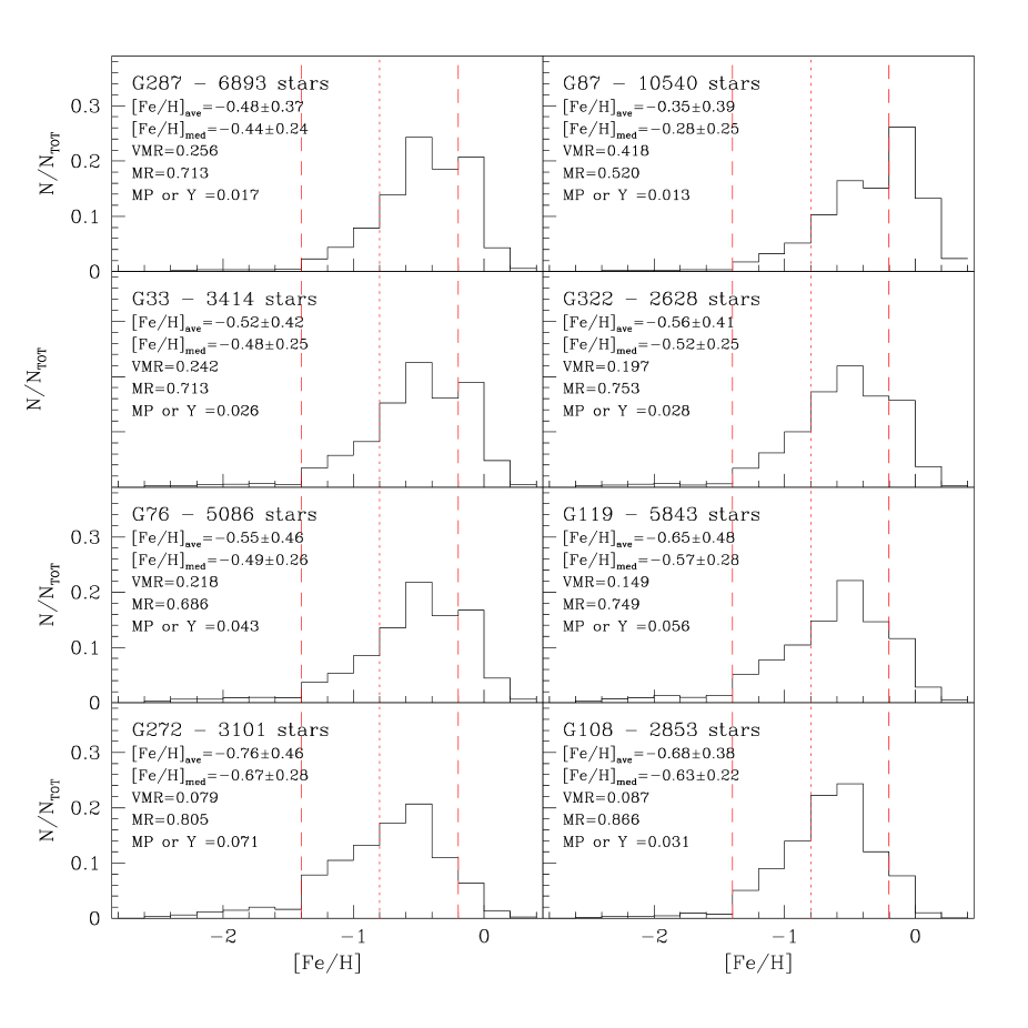
Figure 14: Histograms of the metallicity distributions, in the Carretta & Gratton (1997) scale, for the fields: G287, G87, G33, G322, G76, G119, G272 and G108. In the upper left corner of each panel are reported: the name of the field, the number of stars used to derive the MD, the average metallicity ($[Fe/H]_{ave}$) together with the associated standard deviation, the median metallicity together with the associated semi-interquartile interval, and the fractions of stars with: $\rm[Fe/H]<-1.4$ [Metal-Poor or Young–MP or Y], $\rm-1.4<[Fe/H]<-0.2$ [Metal-Rich –MR], $\rm[Fe/H]>-0.2$ [Very Metal-Rich – VMR], respectively.

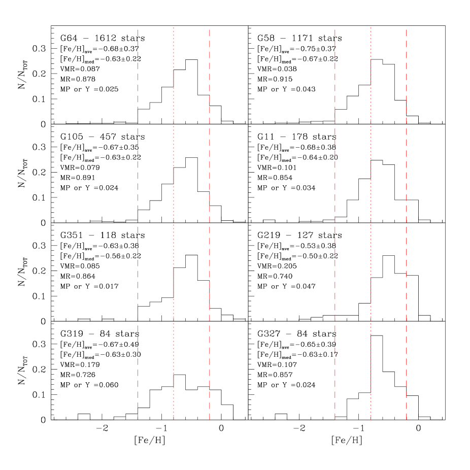
Figure 15: The same as Fig. 14 for the fields: G64, G58, G105, G11, G351, G219, G319 and G327.

Based on the ridge lines, the distance moduli and the reddenings of the template clusters listed in Table 3, and on the assumptions we have made about the distance modulus and reddening of M31 (Sect. 4.2), we have derived the metallicity distributions for all the individual fields shown in figures 14 and 15 in the same order as in figures 5 and 6.

In each panel is reported: the name of the field, the number of stars used to derive the MD, the average metallicity ($\rm[Fe/H]_{ave}$) together with the associated standard deviation, the median metallicity together with the associated semi-interquartile interval, and the fractions of stars with $\rm[Fe/H]<-1.4$ [Metal-Poor or Young – hereafter: MPorY], $\rm-1.4<[Fe/H]<-0.2$ [Metal-Rich – MR], and $\rm[Fe/H]>-0.2$ [Very Metal-Rich – VMR], respectively (see below).

The most striking property of the MDs shown in figures 14 and 15 is their overall similarity. To describe them in a quantitave way (without ”forcing” the analysis beyond a certain level of speculation), after several different tests we decided that the best solution would be to schematically subdivide the histograms into three main intervals as indicated by the vertical lines drawn in the plots presented in Fig. 14 and 15:

• $\rm[Fe/H]<-1.4$, the Metal-Poor or Young group – MPorY

• $\rm-1.4<[Fe/H]<-0.2$, the Metal-Rich group – MR

• $\rm[Fe/H]>-0.2$, the Very Metal-Rich group – VMR

The values of –1.4 and –0.2 were chosen because they mark either a discontinuity in the MDs (at –1.4), or a discontinuous behaviour of the metal-rich tail (at –0.2).

The long ”thin” tail reaching metallicities as low as $\rm[Fe/H]<-2.5$ could be interpreted as due to: (a) very metal-poor old stars truly representative of the old halo of M31, though at a trace level, and/or (b) young blue stars which mimic a metal poor population, especially in the inner disk fields. This is the reason why we have called this group MPorY.

On the opposite extreme of the distributions, in the VMR-regime, at $\rm[Fe/H]=-0.2$, especially in some fields (e.g. G287, G87, G33, G322, G76, G219, G319), one can see a second discontinuity (variable in size from field-to-field) which could be ascribed to the existence of a very metal-rich component, added to the metal-rich tail of the bulk population.

In a few fields (i.e. G108, G58, G351, G219, G327) one might also see another discontinuity at $\rm[Fe/H]\sim-0.8$. However, taking into account the quoted intrinsic uncertainties and the possible effects induced by the binning size, we are inclined to adopt just two cuts. We will discuss in a specific section (sect. 9.3) the results of dividing the total sample in two sub-samples only, cutting at $\rm[Fe/H]\sim-0.8$.

Before summarizing it may be useful to note that we do not report the results of any multi-gaussian fitting to the data, as we found that the degree of discretionality in setting the several parameters (number of components, metallicity limits, widths, etc.) is rather high compared to the intrinsic quality of the available data.

In synthesis all the fields:

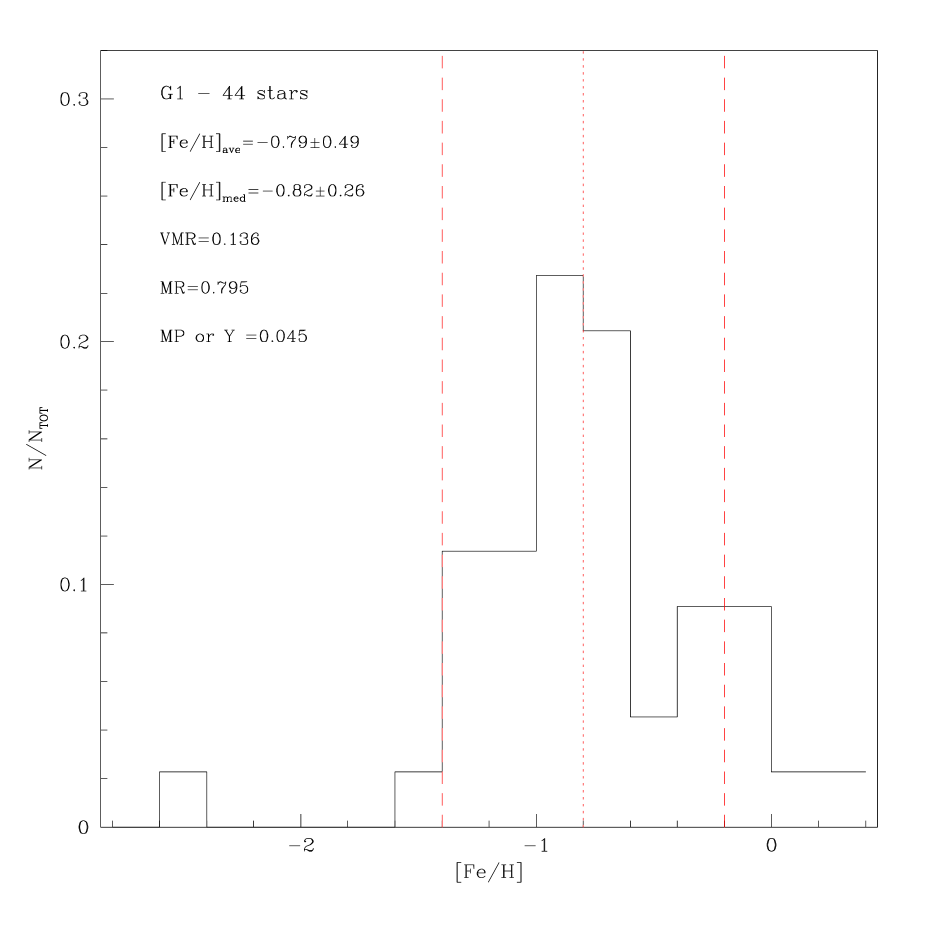
Figure 16: The metallicity distribution (same as Fig. 14, 15) for the field adjacent to the remote globular cluster G1, 35 kpc from the M31 nucleus. The frames from Rich et al. (1996) have been reduced in the same way as all other fields in our dataset.

• have the bulk of the population located within the central metallicity interval, i.e. $\rm-1.4<[Fe/H]<-0.2$, with an obvious main peak around $[Fe/H]\simeq-0.6\pm 0.20$. Most of the fields in Fig. 15 are so distant from the disk as to be true halo fields, yet the metal rich peak is the most evident feature of the distribution, and the fraction of stars with $\rm[Fe/H]<-0.8$ ranges from only 0.1 to a maximum of 0.4 (see Table 5). To test further this point, we reduced the frames used by Rich et al. (1996) and derived the calibrated photometry of the field of the remote cluster G1 ($R_{arcmin}\sim 150$), with the same pipeline adopted for all fields presented here. The resulting CMD is virtually identical to that presented by Rich et al. (1996). In Fig. 16 it is shown that the MD of this extreme region of M31 is very similar to that of the other inner fields. In particular, the mean metallicity is still as high as $\rm[Fe/H]=-0.8$.

• show a long, poorly populated tail spanning the metallicity interval $\rm-2.5<[Fe/H]<-1.4$. As one can see in Fig. 8, stars bluer (more metal-poor) than the ridge line of G11 ([Fe/H] $\sim$ -1.9) do exist and have been detected in all fields at the level of a few percent of the total sample. These stars are probably representative of the very metal-poor old halo of M31 in the outer, less disk contaminated fields. In the inner disk-dominated regions this subsample most probably includes blue young stars which in our procedure (based on colors) may mimic metal-poor objects.

• show a significant population of stars with $\rm[Fe/H]>-0.2$, varying with distance along the Y-axis from $\sim 40$% in the most central fields to less than $\sim 4$% in the most distant ones, with a few exceptions (e.g. G219).

• the field of G219 stands out in that its VMR pupolation is stronger than might be expected from its location, and the distribution looks qualitatively different from the others. As discussed later and shown in Fig. 20 , this field is well superposed on the metal rich tidal tail found by Ibata et al. (2001) and Ferguson et al. (2002) (their Fig. 7). It is interesting to note that the abundance range of this field is similar to those located at large galactocentric distance, only the prominence of the VMR peak is greater.

  A similar behaviour, albeit with a much wider MD and a less pronounced peak, might be present in G319 located not far from the quoted stream (see Fig. 20).

Table 4 reports the populations of each metallicity bin (step 0.2 dex) for each field to make available to the reader the grid of the MDs for further analysis.

6.2.1 Is our Very Metal-Poor population real?

As mentioned earlier, metal poor stars are expected to be present, based on the existence of a blue HB. If the metal poor tail were mostly due to contaminating younger stars it would be expected to reach its minimum extent in the most external halo fields where no such stars are expected to be present. However, the fraction of blue objects seems to be fairly constant ($\sim 2-5$%), so we are inclined to interpret them as truly old and very metal-poor stars.

Independent confirmation of the existence of metal-poor halo giants has been provided by the recent work of Reitzel & Guhathakurta (2002) based on Keck/LRIS spectra. ¿From a preliminary sample (obtained from a $16\times 16$ arcmin² field located at $R=1.6\deg$ on the M31 minor axis), they selected 24 bona fide M31 RGB stars on the basis of their position in the CMD and their radial velocity, and derived metallicity estimates from the strength of the Ca II lines. 21 of the selected RGB stars have $[Fe/H]\leq-1$, 17 of them have $[Fe/H]\leq-1.5$ and some reach metallicity of $[Fe/H]\sim-2.5$ or lower. The result is independent of the assumed metallicity scale. So metal poor stars are indeed present in the M31 halo and are not rare.

6.2.2 Is our Very Metal-Rich population real?

As already noted by simple visual inspection of the CMDs, it is quite evident that, at any level of magnitude, a good number of stars redder than the ridge line of NGC 6553 ($[Fe/H]=-0.16$) is present almost in all fields, and varies from field-to-field depending mostly on galactocentric position.

These objects cannot be accounted for by photometric blends or by any other conceivable photometric effect. There is also no indication to suspect that they are not members of the M31 system. If this is true, this population of stars does exist in these fields, and should have a very high metal content given its location in the observed CMD.

However, due to the combined effects in the (I,V-I) plane of factors like e.g. (a) the V,I limiting magnitudes, (b) the saturation for the brightest stars, (c) the increasing bending and separation, and the non-monotonic behaviour of the ridge lines with increasing metallicity, (d) the possible existence of patchy differential reddening, and (e) the uncertainties in the adopted metallicity scale that are larger at the high metallicity end, it is very difficult to assign a precise value of metallicity to these objects. Both the value of their absolute average metallicity and, especially, the detailed distribution over smaller metallicity bins are very uncertain and need a much better and deeper analysis, probably not feasible via photometric means.

Harris et al. (1999) and Harris & Harris (2000, 2002) find the same result for the halo of NGC 5128. Interestingly, both the metal poor and metal rich peaks they find in NGC 5128 are identical to those in the halo of M31.

We emphasize again that any abundance estimate depends on the choice of the calibrating templates. The suggestion of sub-structures and a fit to the Simple Model of chemical evolution discussed by Harris & Harris (2000, 2002) are tantalizing, but we caution that the present abundances are not sufficiently accurate to allow firm astrophysical conclusions with such detail.

7 Effect of varying assumptions on the MDs

Metallicity determinations obtained via purely photometric data (i.e. stellar/population colors) are strongly dependent on various assumptions and uncertainties in fundamental issues such as (for known/assumed population age) the choice of the metallicity scale, the reddening and the distance modulus.

We explored these effects by re-deriving the MD of a test field (G64) under a set of different assumptions for the metallicity scale, the distance modulus and the reddening. The results of this test are shown in Fig. 17. It may be useful, however, to discuss in some detail the possible impact of each parameter, separately.

7.1 The metallicity scale

Panels (a) and (b) in Fig. 17 show the MD derived for G64 using our standard assumptions, and the CG and ZW metallicity scales, respectively. Our major conclusions are unaffected if we simply shift by about –0.2 dex (i.e. the offset between the two scales at mid-metallicity range) the adopted metallicity boundaries (from -1.4 to -1.6, and from -0.2 to -0.4) when passing from CG to ZW.

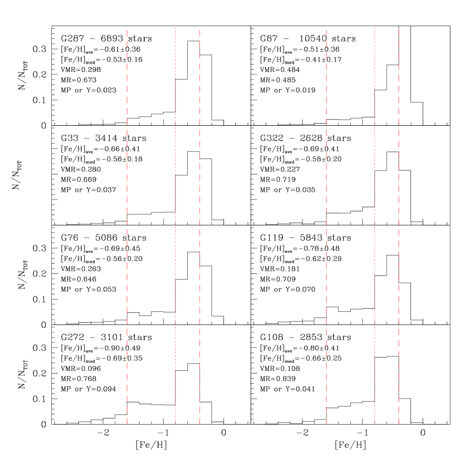
Figure 18: Histograms of the metallicity distributions, in the Zinn & West (1984) scale, for the fields: G287, G87, G33, G322, G76, G119, G272 and G108. In the upper left corner of each panel are reported: the name of the field, the number of stars used to derive the MD, the average metallicity ($[Fe/H]_{ave}$) together with the associated standard deviation, the median metallicity together with the associated semi-interquartile interval, and the fractions of stars with: $\rm[Fe/H]<-1.6$ [Metal-Poor or Young–MP or Y], $\rm-1.6<[Fe/H]<-0.4$ [Metal-Rich –MR], $\rm[Fe/H]>-0.4$ [Very Metal-Rich – VMR], respectively.

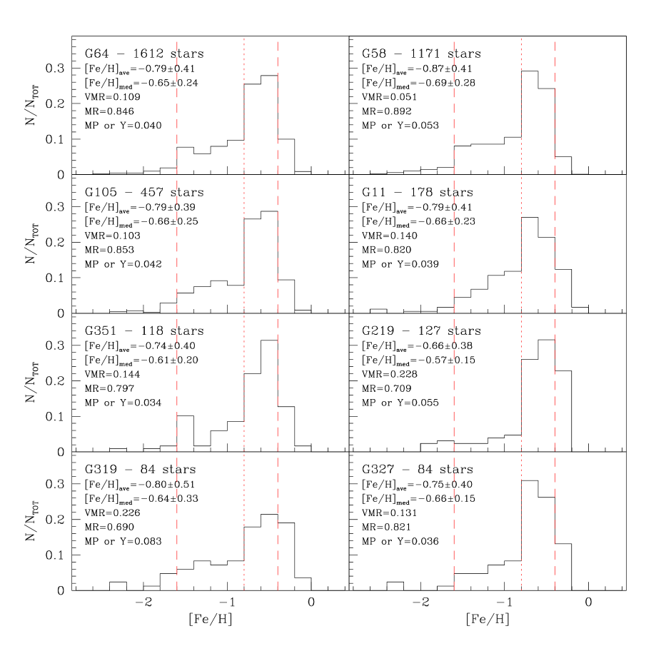
Figure 19: The same as Fig. 18 for the fields: G64, G58, G105, G11, G351, G219, G319 and G327.

In particular, we see that both sets of MDs show a poorly populated tail reaching as far as $[Fe/H]<-2$. The use of the ZW scale does not affect the median of the MD, which remains at [Fe/H] $\sim-0.6\pm 0.1$, but it shifts the average by about $-0.13$ dex. A possible additional peak at $[Fe/H]\sim-1.5$ dex seems to emerge. The evidence for the very metal-rich (VMR) component remains, though shifted by one bin. In fact, a large fraction of the VMR objects in the ZW-scale (see figures 18, 19) are found within the interval $-0.4<[Fe/H]<-0.2$ due to the non-linear relationship between the two metallicity scales.

Given the importance of this issue, we have then derived the MDs for all fields using the ZW scale, to ease the comparison with the previous studies. Figures 18 and 19 show the resulting distributions for all the considered fields. We note that:

• the bulk of the population is metal-rich and peaks at $[Fe/H]\sim-0.6$, as with CG;

• the young/metal-poor population (MPorY) is well detectable and perhaps even enhanced, displaying a slightly bumpy feature whereas the use of the CG scale produces a smoother metal-poor tail;

• a significant very metal-rich population with $[Fe/H]>-0.4$ is clearly present, though the separation from the metal-rich side of the ”central” component is sligtly less clear. We also note that a large fraction of these metal-rich objects populate the bin -0.4, -0.2, due the already mentioned different behaviour of the two metallicity scales in the very metal-rich regime.

• the percentage of the VMR stars varies from field-to-field as with the CG-scale; G219 is confirmed to be peculiar.

In summary, the only possible (and very marginal) difference between the two sets of results is the slightly different appearance of the MDs in the metal-poor range, that could be interpreted as an indication for the existence of a possible secondary peak at $[Fe/H]_{ZW}$ $\sim-1.5$ in a few fields. However, we do not attach much weight to this interpretation, since this might be due to, or enhanced by, a slight discontinuity in the behavior of the RGB colors as a function of [Fe/H]_ZW in the template grid, that occurs at [Fe/H]_ZW $\sim$ –1.4. This discontinuity is not present in the CG scale.

We note again that the choice of a different metallicity scale does not make any dramatic difference in the results, at least at the level of detail we believe is compatible with the intrinsic quality of the available data.

7.2 The distance

The panels (c) and (d) in Fig. 17 consider the effect of varying the M31 distance modulus by $\pm 0.15$ mag on the MD of G64. This variation is rather large and must be considered an upper limit, yet the variation induced on the mean and mode of the metallicity distribution is only $\pm 0.07$ dex.

Also the variation induced on the relative contributions of the three possible components defined by the three metallicity regimes (Sect. 6.2) is quite small.

7.3 The total reddening

The effect of a total reddening variation of $\pm 0.05$ is not negligible, producing a variation of $\pm$ 0.13 dex on the mean and mode of the MD, and, consequently, would alter quite significantly the relative contribution of the smaller components (i.e. MPorY, VMR) to the global abundance distribution. However, the blue locus of the RGB, along with other estimates of the reddening toward M31, constrain the reddening of our fields well within this range.

As already noted, since within the adopted approach the MDs are fully drawn from the distributions of the intrinsic colors translated into MD via the adopted grid, it is unavoidable that any systematic shift of the colors correspondingly affects the MDs. And, since the relationship between color and metallicity is highly non-linear, even a small variation of the adopted reddening (at the level of a few hundredths of a magnitude) induces both a shift and a deformation of the MDs, especially in the metal-poor regime where the sensitivity to color variation is much larger. Note however that the median and mean metallicity estimates do not vary more than $\pm 0.2$ dex in response to a $\pm 0.05$ change in reddening.

7.4 Conclusions from the Tests

The results of the above tests can be summarized as follows:

i) With any plausible choice of distance modulus and total reddening, most of the stars (i.e. $\sim 60-80$% of the total) lie in the range $\rm-1.4\leq[Fe/H]\leq-0.2$ and the peak of this main component of the MD lies between $\rm[Fe/H]=-0.8$ and $\rm[Fe/H]=-0.4$, independently of the metallicity scale.

ii) Although the existence, as distinct populations, of two additional components at the very metal-poor and very metal-rich ends of the MDs may be debatable, the existence of very metal poor stars (also supported by the presence of a BHB population) and of very metal-rich stars seems to be quite firmly established.

iii) As repeatedly noticed, the uncertainties in deriving abundances from photometry are still rather large, and settling the question of whether the abundance distributions are merely skewed or bimodal or even tri-modal will require much more accurate and reliable means of metallicity determinations, e.g. better photometric data coupled with a more reliable and extended grid of reference GC or the availability of spectroscopic data for a wide sample of stars.

8 Comparison with other MDs in the literature

Several authors have investigated M31 fields using both ground-based facilities and $HST$ observations. We here compare our present results with those of the most recent previous analyses, noting that all of them work in the ZW metallicity scale.

• Holland et al. (1996)

  These authors studied the halo fields near G302 and G312, located 32 and 50 arcmin approximately along the SE minor axis, respectively. The reddening and distance modulus assumed for M31 were $E(B-V)=0.08\pm 0.02$ and $(m-M)_{0}=24.3\pm 0.1$. The RGBs were compared with the RGB ridge lines for three Galactic GCs (i.e. M15, NGC1851 and 47 Tuc) and two metal-rich fiducials selected from isochrones with age $t_{0}=13.8$ Gyr and [m/H]=–0.4 and 0.0. The resulting MDs show a spread in metallicity of $-2\leq[m/H]\leq-0.2$ with the majority of stars having $[m/H]\sim-0.6$.

  We have not analysed these fields, but we can compare these results with ours on halo fields such as G105 and G319. The $(V-I)_{0}$ color distribution of the RGBs at the approximate level I $\sim$ 22.45 (i.e. $M_{I}=-2.0$) seems to peak around 1.25 $\pm$ 0.2, at a cursory inspection of their Fig. 2 and 3; the resulting MDs are in very good agreement with our results, both in the shape and in the location of the MD peak at $[Fe/H]\sim-0.6$.

• Sarajedini & Van Duyne (2001)

  The disk-dominated field near G272 was recently analysed by Sarajedini & Van Duyne (2001), who derived a MD for it. Their analysis is based on the assumptions that $E(B-V)=0.08$ and $(m-M)_{0}=24.5$ for M31. Their fiducial sequences are the RGB ridge lines of 6 Galactic globular clusters and one open cluster, of which only 47 Tuc is in common with our grid.

  The interpolation procedure, similar in principle to ours, was applied within a narrow range of magnitude along the RGB, i.e. I=22.65 $\pm$ 0.1 corresponding to $M_{I}=-2.0\pm 0.1$ mag. The $(V-I)_{0}$ color distribution within this strip (Fig. 6 in Sarajedini & Van Duyne (2001)) has a Gaussian shape peaking at $(V-I)_{0}\sim 1.4$, whereas the color distribution we derive from our data under our assumptions peaks at $(V-I)_{0}\sim 1.2$. This difference is largely accounted for by the different choice of reddening; differences in the absolute calibration (e.g., aperture corrections) may also contribute.

  The MD obtained by Sarajedini & Van Duyne (2001) is similar in shape to ours, with an extended metal-poor tail reaching [Fe/H] $\leq$ –2, but their main peak at [Fe/H] $\sim$ –0.2 is definitely shifted by about 0.2 dex toward the metal-rich end. This is at least partly due to the quoted systematic difference in the color distribution.

  On this basis, these authors conclude that their Gaussian component peaking at $<[Fe/H]>=-0.22\pm 0.26$ comprises $70$ % of the total number of stars in the sample, and is attributed to the thick-disk population.

  We cannot compare this result homogeneously with ours because we have not fitted our MD with Gaussian components: however, we note that the fraction of very metal-rich stars with [Fe/H] $\geq$ –0.4 is $\sim$ 10% in the ZW scale (see Fig. 18 and Table 5), which is not unusually large and is quite consistent with the position of G272 with respect to the major axis of M31. If indeed we are observing the thick-disk population in this field, its relative contribution is not overwhelming and is found also, and to a larger extent, in all the other fields located on the disk of M31 (see Sect. 9).

• Ferguson & Johnson (2001)

  The far outer disk field near G327 was recently investigated by Ferguson & Johnson (2001). Under the standard assumptions of E(V–I)=0.10 and $(m-M)_{0}$=24.47, the RGB was compared with the fiducial ridge lines of three GGCs in the metallicity range –1.9 to –0.3. A best fit was performed at the luminosity level $M_{I}=-0.13\pm 0.1\leavevmode\nobreak\ mag$, consistent with a predominantly old-to-intermediate age stellar population with [Fe/H] $\sim$ –0.7 plus a trace population of old metal-poor stars.

  In this field we also find a MD with a median value at [Fe/H] $\sim$ –0.66 (ZW-scale), and only $\sim$ 20% of stars with [Fe/H] $<$ –0.8.

• Durrell et al. (2001)

  An outer halo field located 90 arcmin (i.e. 20 kpc) SE of the M31 nucleus and roughly along the minor axis was studied by Durrell et al. (2001) using CFHT V,I data. A reddening value $E(V-I)=0.10\pm 0.02$ was derived from the color distribution of the foreground Milky Way halo stars, and a distance modulus $(m-M)_{0}=24.47\pm 0.12$ was derived from the luminosity of the RGB tip.

  A cursory inspection of their Fig. 7 indicates that the RGB stars at V $\sim$ 22.6 (corresponding to $M_{I}\sim-2$) populate a (V–I) color range between approximately 0.9 and 1.6 with a presumable accumulation between 1.2 and 1.4.

  The MD functions are derived by comparison with evolutionary tracks for 0.8 $M_{\odot}$ stars. The MD for the RGB magnitude interval 20.6 $<$ I $<$ 22.5 is skewed toward the metal-poor side reaching almost [m/H]=–2.5, and could be well fitted by two Gaussian components peaking at [m/H]=–0.52 and –1.20 and including 60% and 40% of the total stellar population, respectively. The agreement with our analysis of the distant fields G105 and G319 is quite satisfying (see Tables 4 & 5).

• Reitzel & Guhathakurta (2002)

  A spectroscopic study based on Keck-LRIS data of about 30 halo red giant stars in a field at R=19 kpc on the SE minor axis of M31 was done by Reitzel & Guhathakurta (2002). The MD they find for these halo giants spans more than 2 dex range with a mean/median value [Fe/H] $\sim$ –1.9 to –1.1 (depending on calibration and sample selection). However, the high metallicity end of this distribution is poorly constrained by these data since the selection function for secure M31 members excludes $>$ 80% of the giants in solar/super-solar metallicity range.

  No direct comparison is possible with our results, except for a general comment on the confirmation of the existence of a well-detectable fraction of metal-poor stars in the outer halo of M31 (see Sect. 6.2). Our field G319 is within $\sim$ 30 arcmin of their field on the minor axis, and we do observe the MR population found in other fields.

9 Correlation of metallicity with position

9.1 The wide-field survey by Ferguson et al. (2002)

In a very important photometric survey of the halo and outer disk (appeared when the present analysis was nearly completed), Ferguson et al. (2002) have studied in great detail both the spatial density and metallicity variations (as inferred from color information, like in the present paper), covering an area of about 25 square degrees around M31. This is by far the most detailed and complete ground-based study carried out so far on the field population in M31.

Since the CCD data were obtained with the 2.5m INT-WFC at La Palma, the limiting magnitudes (with $S/N=5$) are V=24.5 and $i=23.5$, much brighter than those we have obtained from our $HST$ photometry. The shallower limits in magnitude are however amply balanced by the much wider area sampled. Therefore this survey and our work from $HST$ data are nicely complementary.

Their conclusions, very convincingly supported by their fig. 2-7, are schematically:

• There is evidence for both spatial density and metallicity variations across the whole body of M31, which are often, but not always, correlated.

• Besides the known Ibata’s stream, two other overdensities at large radii can be detected, close to the SW major axis, in the proximity of the very luminous GC G1 (called the ”G1-clump”), and near the NE major axis, coinciding with and extending beyond the previously known ”northern spur”.

• The most prominent metallicity variations are found in two large structures in the southern half of the halo, the first one coinciding with the giant stellar stream found by Ibata et al. (2001), and the second one corresponding to a much lower stellar overdensity. Their metallicities are above the average value, which corresponds approximately to that of 47 Tuc, i.e. $[Fe/H]\sim-0.7$.

Since the areas covered by the previous studies are very small compared to this wide survey, as correctly pointed out by Ferguson et al. there is no ground to identify significant conflicts between the results of previous studies on individual fields and those derived from this general panoramic study. This is especially true because of the clear detection of streams and substructures (both in star density and metallicity) allover M31, which has made somehow ”unpredictable” the nature of the population one would expect to find on the basis of the mere X,Y location within M31.

This fact has an obvious impact on the general interpretation we might derive from our analysis, as the lines of sight we have investigated, though quite numerous (16 + G1), could be not sufficiently representative of the global scenario.

In this new light we have reconsidered the properties of our observed fields, with particular attention to the map of the spatial and chemical substructures Ferguson et al. (2002) presented in their Fig. 7, and reported here in Fig. 20 where the locations of our fields are overplotted. We anticipate that the results coming out from our deeper $HST$ fields suggest that indeed some of the considered lines of sight may be affected by the presence of streams and overdensities.

9.2 Our 16+1 $HST$ fields

As reported in figures 14 and 15 and Table 4, a number of parameters have been derived from the metallicity distributions for each field. A straightforward application is to check first for any trend with position in the galaxy, recalling the already quoted caveat that only projected distances are available.

9.2.1 The (X,Y)–plane

Fig. $21a,b,c$ report the fractions of MPorY and VMR stars as a function of the X and Y coordinates and galactocentric distance R in arcmin, respectively. The error bars associated to each point are based on the square roots of the star numbers in each individual sample.

Because of the large difference in the error bars associated to the different fields, as the respective population size ranges from about 10,000 stars in the inner fields down to less than 100 in the outer halo fields, it is quite hard to assign a fair statistical significance to any trend one might see. Nevertheless, considering also the histograms presented in figures 14 and 15, some general comments can be made:

• The fraction of MPorY stars is substantially constant and independent of position. As already noted, this does not necessarily mean that there is a constant percentage of metal-poor halo stars in all the observed fields, because of the possible (and, at the present status, unknown) contamination by Young objects in the inner samples. However, metal-poor old stars are surely present in the halo, albeit in rather small quantity.

• The inner fields (G87, G287) have a population with a higher average metallicity than all other fields, resulting from the combination of a higher than average VMR fraction and a (correspondingly) smaller MR fraction (remember that the total MPorY + MR + VMR = 1.0). This evidence is especially clear looking at the Y-plot (Fig. 21b).

• Ferguson et al. (2002) noted that the average metallicity of the SW fields (i.e. with negative Y and negative X) is slightly larger than the average metallicity estimated for the NE fields. Though the statistical significance is weak, this effect is perhaps visible also in Fig. 21a,b, as a slight enhancement of the mean fraction of VMR stars in the $Y<0$ and $X<0$ regions.

• G219 and G319 have an unusually large fraction of metal-rich stars for their distance from the M31 center (90 and 70 arcmin respectively). This anomaly may be connected with their (projected) proximity to the Ferguson et al. (2002) stream.

In summary, the considerations reported above show that a simple description of the results making use of just the $HST$ fields and their projected location in the X.Y-plane coupled with a ”simple” description of the M31 outer disk and halo may be not fully capable to extract all the information potentially offered by the available data.

This has prompted us to look at our result within the new scenario emerging from Ferguson et al. (2002) work.

9.2.2 HST fields and detected substructures

If we briefly rediscuss our data within the framework reported in Fig. 20 (where the fields are identified over the cartoon reproduced from Fig. 7 of Ferguson et al.), we can add some further notes:

• Several fields (e.g. G33, G219, G105, G58, G64, G108) are located or projected on the ”giant stream” first identified by Ibata et al. (2001) and now confirmed by Ferguson et al. (2002).

  Some of these fields (see Table 4,5) show a very high fraction of VMR stars, with a clear peak in the MD. The G219 field presents one of the best examples of this case. G219 is located well off the plane but lies precisely on the detected stream; the field has an anomalously large fraction ($\sim 20$%) of very metal rich stars.

  Though one cannot conclude for sure that the existence of these VMR stars in most of these fields has to be ascribed to the possible physical connection with the ”giant stream”, it seems conceivable that the two facts may be related. On the other hand, there are also fields that are located/projected on the stream which do not show a similarly evident ”excess” of VMR stars (see f.i. G58, G64, G105).

• The MD of G1 may also be worth of a short comment within the new scenario. In fact, even though it is a distant field (projected some 32 kpc from the nucleus) and with a total population of measured stars of only 44 objects, its MD shows (see Fig. 16) a weak indication for a second metal-rich peak (at $[Fe/H]\sim-0.2$, with F(VMR) $\sim 10$%.

  Since, as shown in the map in Fig. 20, the region called by Ferguson et al. the ”G1 clump” denotes a possible substructure (at least in star density) within the area they surveyed, it may be of some relevance to investigate further the existence and origin of VMR objects in this field.

In summary, the re-analysis of the properties of the MDs within the framework provided by Ferguson et al. (2002) does not yield a fully satisfactory ordering and detailed explanation for all the fields investigated in the present study. However, some (otherwise unusual) results are nicely fitting (or, at least, are compatible with) a scenario that accounts for the existence of significant substructures within M31. These may add an important piece of information for a detailed description of the formation and evolution of this galaxy, including the possible interaction with close companions such as M32 (Bekki et al., 2002; Choi et al., 2002).

9.3 Large-scale trends

In the previous sections we have carried out and discussed the analysis of the MDs we have obtained from the histograms shown in figures 14 and 15 assuming that, independently of the physical reasons or adopted models for M31, one could identify two features or discontinuities, at $[Fe/H]=-1.4$ and $[Fe/H]=-0.2$, to separate the stars into three main groups. We are quite confident that such an approach is meaningful and the considerations listed above add some support to this.

An alternative and more schematic approach could be simply to consider two groups of stars obtained by dividing the total MDs for instance at $[Fe/H]=-0.8$.

This value for the cut has been chosen to identify roughly what we call hereafter the “Metal-Rich Population” (MRP) from the “Metal-Poor Population” (MPP) on the basis of the already quoted (weak) evidence of a small discontinuity in the MDs at that bin-border (deduced from inspecting the histograms, see f.i. G33, G322, G108, G58, G351, G219, G327; see also Fig. 12).

Table 5 reports for each field the values so obtained from the histograms for the fraction of the Metal-Poor Population , F(MPP), and the Metal-Rich Population, F(MRP), the Y-coordinate, and the average (median) metallicity of the total sample.

Fig. 22 a,b shows the plots of F(MPP) and of the median metallicity vs. the absolute Y-coordinate, respectively.

As said, the contribution of stars from the spheroid is expected to grow faster along the Y-direction because of the inclination of the M31 disk with respect to the plane of the sky.

In fact, F(MPP) grows very rapidly from 0.10 at $|Y_{arcmin}|\sim 0$, to $\sim 0.45$ at $|Y_{arcmin}|\sim 17$, showing a good correlation between the involved variables. However, from $|Y_{arcmin}|\sim 20$ to $|Y_{arcmin}|\sim 70$, F(MPP) remains nearly constant at F(MPP)$\sim 0.4$, with a larger scatter. Note that the two “outliers” with low values of F(MPP) at quite large Y are G219 and G351, both located on or near the ”giant stream” (see Fig. 20). A similar behaviour is shown by the median metallicity (Fig. 22b)

The trend displayed in figures 22a and 22b is quite clear: the MRP dominates the inner region but the relative importance of the MPP population rapidly grows going far from the visible disk. However, in the explored range of $|Y_{arcmin}|$, the Metal-Poor population never becomes dominant, Metal-Rich stars remain the major component of the stellar mix.

In summary, these plots suggest that, besides the existence of important substructures, there is also evidence of a more regular pattern in the inner parts of the galaxy, possibly testifying of a relatively homogeneous and ordered formation process, later perturbed by merging events.

10 Summary and Conclusions

We have analysed HST-WFPC2 images of 16 fields in M31 at a wide range of distances from the galactic center and plane. These fields have been observed in the F555W (V) and F814W (I) filters and reach a roughly uniform depth.

The color-magnitude diagrams of these fields are generally dominated by a red giant branch and a populous red clump. The RGB has a strong descending tip, indicative of a metal rich population. In the outermost fields a blue Horizontal Branch is also detected. When present, the blue HB represents about 15% of the total HB population, roughly estimated from the fraction of metal poor giants.

In fields superposed on the disk, a blue plume of main sequence stars is also identified. We report a simple analysis of the blue plume population, which shows that the star formation history of the disk has been spatially inhomogenous during the last 0.5 - 1 Gyr.

We have obtained photometric metallicity distributions from RGB stars by interpolation on a grid of empirical globular cluster RGB templates.

The most robust result of the present $HST$ survey is the evidence that the metal-rich population, with $[Fe/H]\sim-0.6$, is the major component of the stellar mix everywhere in the $10\leq R_{arcmin}\leq 130$ range. A minor metal-poor component (with $[Fe/H]<-1.4$) is also ubiquitous. The old stellar population is remarkably uniform across the disk, outer halo fields, and in the proposed tidal stream. This uniformity is the dominant feature of the old stellar population.

This basic result is not new (see, e.g., Durrell et al., 2001, and references therein), but coupled with data shown by the very wide mapping carried out by Ferguson et al. (2002), fixes on solid grounds the conclusion that the stellar population of the M31 spheroid differs substantially from that of the Milky Way and is almost an order of magnitude more metal rich, on average. In this respect, we confirm also the finding of Rich et al. (1996), that the metal rich population is present even at 150 arcmin ($\sim$ 35 kpc) from the nucleus, at the location of the globular cluster G1.

An obvious explanation for the origin of the metal rich halo of M31 is that the population formed in connection with the outflow of metal-enriched winds, perhaps associated with the formation of the spheroid. Metal rich populations in halos are clearly widespread (e.g. NGC 5128; Soria et al., 1997; Harris et al., 1999; Harris & Harris, 2002). There is evidence for the outflow of metal enriched winds in Lyman break galaxies, and for near-solar abundances in these galaxies, at high redshift (Steidel et al., 1996). The stars formed from this material might well live to comprise the population II halo. The outflow of enriched material will not affect the shape of the abundance distribution (the classic Simple Model form is retained) but the yield (mean abundance of the whole galaxy) does decline (Hartwick, 1976).

The increasing fraction of the ”Metal-Poor Population” (i.e. with $[Fe/H]<-0.8$) with distance from the plane Y suggests a dissipational origin for the regions that are closer to the galactic plane. This evidence is compatible with the hypothesis that a ”homogeneous” formation event may have occurred in the very early stages of the M31 history.

On the other hand, the image of the M31 halo illustrated by Ibata et al. (2001) and Ferguson et al. (2002) shows (for the metal-rich stars taken as a global population) a quite flattened, disk-shaped distribution, associated with the outskirts of the inner disk. It is possible thus that the metal rich population might be associated with a proto disk or flattened halo. The large number of stars involved would strongly favor the notion that we study the old disk, and not just some trace population such as the thick disk. So we have this alternative scenario, where the dominant metal-rich population might be associated with a meta-disk extending perhaps more the 20 kpc, while the metal-poor population might be associated with the spheroid. The two populations – and the corresponding structures – would have different evolutionary histories. The old stellar disk would be much larger than previously believed, extending out to a few degrees from the nucleus of M31 and dominating the stellar mix also along lines of sight very distant from the center of the galaxy (Ferguson & Johnson, 2001; Ferguson et al., 2002). It is also possible that the inner disk and bulge had common, or closely tied, formation histories.

In addition to this, the sub-structures (“streams” and “clumps”) clearly detected by Ibata et al. (2001); Ferguson et al. (2002) and supported by our results might be related to the phenomena of merging or interaction with satellites. In this case the metal rich component might be connected with the tidal disintegration of a companion (Ferguson et al. (2002)), a likely candidate being M32, perhaps involving a good deal of its mass (Bekki et al., 2002; Choi et al., 2002).

New data are now required to choose among the scenarios presented here. Deeper HST imaging, some of which is in progress, may constrain the actual age distribution of stars in some regions of the halo. Large scale spectroscopic surveys of halo stars have just begun, and have the potential to determine what fraction of the M31 halo might have originated from the tidal disruption of satellites. Our first round of large-scale HST imaging gives evidence that the old “halo” stellar population is more metal rich than that of the Milky Way, with surprisingly little variation in the properties of the old stellar population, even for fields ranging up to galactocentric distances exceeding 30 kpc. The challenge now will be assemble a data set for the Galaxy and M31 powerful enough to constrain their origins.

Table 1: Location of the observed fields.

G	Bo	Xarcmin	Yarcmin	Rarcmin	E(B-V)	Fsph
G1		$-149.54$	$29.88$	$152.50$	$0.11$	$>0.9$
G11	293	$-61.72$	$43.91$	$75.75$	$0.11$	$>0.9$
G33	311	$-57.58$	$1.24$	$57.59$	$0.11$	$0.07$
G58	6	$-6.80$	$27.37$	$28.20$	$0.11$	$0.70$
G64	12	$-10.65$	$23.01$	$25.35$	$0.11$	$0.65$
G76	338	$-44.15$	$-8.84$	$45.03$	$0.14$	$<0.1$
G87	27	$-26.41$	$1.00$	$26.43$	$0.14$	$0.18$
G105	343	$-57.57$	$-29.81$	$64.83$	$0.11$	$0.80$
G108	45	$7.38$	$20.21$	$21.52$	$0.11$	$0.60$
G119	58	$-28.88$	$-10.06$	$30.59$	$0.14$	$<0.1$
G219	358	$-64.79$	$-58.32$	$87.17$	$0.11$	$>0.9$
G272	218	$17.13$	$-16.88$	$24.05$	$0.14$	$<0.1$
G287	233	$35.44$	$-0.26$	$35.45$	$0.14$	$0.12$
G319	384	$-21.18$	$-68.89$	$72.07$	$0.11$	$0.99$
G322	386	$61.64$	$-4.49$	$61.80$	$0.11$	$0.07$
G327		$130.01$	$5.10$	$130.11$	$0.11$	$>0.9$
G351	405	$63.14$	$-53.71$	$82.90$	$0.11$	$>0.9$

Table 2: Observations.

Name	R.A. (2000)	Dec. (2000)	Date	Proposal	P.I.	Filters (t${}_{exp}[s]$)
G11	0 36 20.78	40 53 36.60	Feb 3,2000	GO 6671	Rich	F814W (5400), F555W (5300)
G33	0 39 33.75	40 31 14.36	Feb 26,1999	GO 6671	Rich	F814W (5400), F555W (5300)
G64	0 40 32.79	41 21 44.65	Aug 17,1999	GO 6671	Rich	F814W (5400), F555W (5300)
G76	0 40 58.83	40 35 47.32	Jan 11,1999	GO 6671	Rich	F814W (5400), F555W (5300)
G87	0 41 14.61	40 55 51.12	Aug 16,1999	GO 6671	Rich	F814W (5400), F555W (5300)
G119	0 41 53.01	40 47 08.63	Jun 13,1999	GO 6671	Rich	F814W (5400), F555W (5300)
G287a	0 44 41.97	41 43 56.40	Sep 26,1999	GO 6671	Rich	F814W (5400), F555W (5300)
G287b	0 44 41.97	41 43 56.40	Sep 26,1999	GO 6671	Rich	F814W (5400), F555W (5300)
G319	0 46 21.92	40 17 00.01	Feb 28,1999	GO 6671	Rich	F814W (5400), F555W (5300)
G322	0 46 26.94	42 01 52.94	Jan 10,1999	GO 6671	Rich	F814W (5400), F555W (5300)
G327	0 49 38.91	43 01 13.85	Jun 19,1999	GO 6671	Rich	F814W (5400), F555W (5300)
G272	0 44 51.40	41 19 16.00	Jan 22,1995	GO 5420	Fusi Pecci	F814W(10800), F555W (3800)
G351	0 49 58.10	41 32 17.00	Jan 18/19,1995	GO 5420	Fusi Pecci	F814W(10800), F555W (3800)
G58	0 40 26.79	41 27 27.72	Feb 15,1994	GTO 5112	Westphal	F814W (2000), F555W (2000)
G108	0 41 43.26	41 34 20.76	Feb 15,1994	GTO 5112	Westphal	F814W (2000), F555W (2000)
G105	0 41 43.17	40 12 22.76	Feb 15,1994	GTO 5112	Westphal	F814W (2000), F555W (2000)
G219	0 43 17.81	39 49 13.53	Feb 15,1994	GTO 5112	Westphal	F814W (2000), F555W (2000)

Table 3: Grid of Galactic Globular Clusters template for metallicity determinations in the Zinn & West (1984) and Carretta & Gratton (1997) scales

	[Fe/H]ZW	[Fe/H]CG	E(B-V)	$(m-M)_{0}$
NGC6341  M92	$-2.24$	$-2.16$	$0.02$	$14.74$
NGC6205  M13	$-1.65$	$-1.39$	$0.02$	$14.38$
NGC5904  M5	$-1.40$	$-1.11$	$0.03$	$14.31$
NGC104  47Tuc	$-0.70$	$-0.70$	$0.04$	$13.29$
NGC6553	$-0.34$	$-0.16$	$0.84$	$13.44$
NGC6528	$-0.23$	$\leavevmode\nobreak\ \leavevmode\nobreak\ \leavevmode\nobreak\ 0.07$	$0.62$	$14.35$

Table 4: Metallicity Distributions in the Carretta & Gratton (1997) scale: population (in percentage) of individual metallicity bins (step 0.2 dex) for each observed field, and for all (coadded) fields.

Name	$<-2.5$	$-2.5$	$-2.3$	$-2.1$	$-1.9$	$-1.7$	$-1.5$	$-1.3$	$-1.1$	$-0.9$	$-0.7$	$-0.5$	$-0.3$	$-0.1$	$0.1$	$.2-.27$	$>.27$
G1	0.0	2.3	0.0	0.0	0.0	0.0	2.3	11.4	11.4	22.7	20.5	4.5	9.1	9.1	2.3	2.3	2.7
G11	0.0	1.1	0.0	0.0	0.6	0.6	1.1	2.2	9.0	17.4	24.7	23.0	9.0	9.0	1.1	0.0	1.2
G33	1.3	0.2	0.2	0.4	0.6	0.7	0.4	3.5	5.8	8.2	15.2	22.5	16.1	19.0	4.8	0.5	0.6
G58	0.4	0.1	0.5	0.5	0.9	1.1	1.2	5.9	11.2	15.5	25.6	23.7	9.5	3.3	0.5	0.0	0.0
G64	0.6	0.2	0.2	0.4	0.4	0.8	0.5	6.0	8.6	14.7	21.5	25.6	11.5	7.3	1.3	0.1	0.5
G76	3.6	0.3	0.6	0.7	0.9	0.9	0.9	3.7	5.3	8.5	13.6	21.8	15.7	16.7	4.4	0.6	1.7
G87	0.4	0.0	0.2	0.2	0.3	0.3	0.4	1.7	3.2	5.2	10.3	16.5	15.1	26.2	13.2	2.3	4.6
G105	0.2	0.0	0.0	0.7	0.4	0.2	1.1	5.0	8.8	15.3	21.9	25.8	12.3	6.8	0.9	0.2	0.4
G108	1.2	0.2	0.4	0.4	0.5	0.9	0.8	5.0	9.0	14.0	22.2	24.4	12.0	7.7	1.0	0.1	0.3
G119	3.9	0.3	0.8	0.9	1.2	1.0	1.3	5.2	7.8	10.4	14.8	22.1	14.6	11.6	2.8	0.5	0.8
G219	0.8	0.0	0.0	0.0	0.8	1.6	2.4	2.4	2.4	7.1	17.3	26.0	18.9	18.1	2.4	0.0	0.0
G272	4.1	0.3	0.6	1.1	1.5	2.0	1.6	7.9	10.5	13.2	17.3	20.7	11.0	6.4	1.3	0.2	0.4
G287	0.5	0.1	0.2	0.3	0.3	0.4	0.4	2.3	4.4	7.9	13.9	24.3	18.6	20.7	4.3	0.6	0.8
G319	0.0	0.0	2.4	0.0	0.0	1.2	2.4	4.8	11.9	13.1	17.9	11.9	13.1	11.9	6.0	0.0	3.6
G322	1.8	0.2	0.3	0.5	0.7	0.3	0.6	3.4	6.2	10.0	17.2	21.9	16.5	15.7	3.7	0.3	0.5
G327	0.0	0.0	2.4	0.0	0.0	0.0	0.0	1.2	8.3	10.7	33.3	19.0	13.1	9.5	1.2	0.0	1.2
G351	0.8	0.0	0.8	0.0	0.8	0.0	0.0	5.9	7.6	9.3	21.2	26.3	16.1	5.1	2.5	0.8	2.5
ALL	1.7	0.2	0.4	0.5	0.7	0.7	0.7	3.7	6.0	9.2	15.0	21.4	15.0	16.8	5.5	0.9	1.7

Table 5: Parameters derived from the Metallicity Distributions in the Carretta & Gratton (1997) scale. Columns: (1) name of the field, (2) fraction of stars with $\rm[Fe/H]<-1.4$ [Metal-Poor or Young – MP or Y], (3) with $\rm-1.4<[Fe/H]<-0.2$ [Metal-Rich –MR], (4) with $\rm[Fe/H]>-0.2$ [Very Metal-Rich – VMR] (5) fraction of stars with $\rm[Fe/H]<-0.8$ [Population Metal-Poor –PMP], (6) fraction of stars with $\rm[Fe/H]>-0.8$ [Population Metal-Rich –PMR], (7) average metallicity ($\rm[Fe/H]_{ave}$) (8) associated standard deviation, (9) median metallicity, (10)associated semi-interquartile interval. The corresponding figures in the Zinn & West (1984) scale are partially reported in Fig. 18 and 19.

Name	$Fr$(MP or Y)	$Fr$(MR)	$Fr$(VMR)	$Fr$(PMP)	$Fr$(PMR)	[Fe/H]av	$\sigma_{av}$	[Fe/H]med	$\sigma_{med}$
G1	0.045	0.795	0.136	0.500	0.477	-0.79	0.49	-0.82	0.26
G11	0.034	0.854	0.101	0.320	0.669	-0.68	0.38	-0.64	0.20
G33	0.026	0.713	0.242	0.200	0.781	-0.52	0.42	-0.48	0.25
G58	0.043	0.915	0.038	0.369	0.627	-0.75	0.37	-0.67	0.22
G64	0.025	0.878	0.087	0.317	0.672	-0.68	0.37	-0.63	0.22
G76	0.043	0.686	0.218	0.218	0.729	-0.55	0.46	-0.49	0.26
G87	0.013	0.520	0.418	0.114	0.837	-0.35	0.39	-0.28	0.25
G105	0.024	0.891	0.079	0.315	0.678	-0.67	0.35	-0.63	0.22
G108	0.031	0.866	0.087	0.311	0.673	-0.68	0.38	-0.63	0.22
G119	0.056	0.749	0.149	0.289	0.664	-0.65	0.47	-0.57	0.28
G219	0.047	0.740	0.205	0.165	0.827	-0.53	0.38	-0.50	0.22
G287	0.017	0.713	0.256	0.163	0.568	-0.48	0.37	-0.44	0.24
G272	0.071	0.805	0.079	0.386	0.824	-0.76	0.46	-0.67	0.28
G319	0.060	0.726	0.179	0.357	0.607	-0.67	0.49	-0.63	0.30
G322	0.026	0.713	0.242	0.224	0.753	-0.56	0.41	-0.52	0.25
G327	0.024	0.857	0.107	0.226	0.762	-0.65	0.39	-0.63	0.17
G351	0.017	0.864	0.085	0.246	0.720	-0.63	0.38	-0.56	0.22
ALL	0.032	0.702	0.233	0.220	0.746	-0.54	0.43	-0.50	0.27

Figure 7: The CMD of the G76 field represented as an isodensity contour plot (Hess diagram) for greater clarity. The main features described in the text are indicated. The outermost countour correspond to a density of 10 stars per $0.1\leavevmode\nobreak\ mag\times 0.1\leavevmode\nobreak\ mag$ box. The step between subsequent contours is 5 up to the 8th contour. The 9th contour corresponds to 75 stars per $0.1\leavevmode\nobreak\ mag\times 0.1\leavevmode\nobreak\ mag$ box and after this contour the step is 100. The innermost contour is at 2200 stars per $0.1\leavevmode\nobreak\ mag\times 0.1\leavevmode\nobreak\ mag$, while the box sampling the peak of the RHB Clump has a density of 2334 stars.

Figure 11: YMS (young main sequence) indices versus deprojected distance from the center of the galaxy (panels a and b), and versus absolute distance along the major axis (panel c). Where no error bars are seen, they are smaller than the symbol size. Only the fields with a substantial YMS population (e.g. disk fields) are plotted. The upper and lower panels plot the total fraction of stars younger than $\sim 0.5$ Gyr as a function of distance from the nucleus, while the center panel shows the fraction of young stars as a function of galactocentric distance. Note that while the G76 field has the strongest young population, it is the sparsely populated G87 field that has the youngest main sequence. The G76 field coincides with a ring of general enhanced star formation 10 kpc from the nucleus.

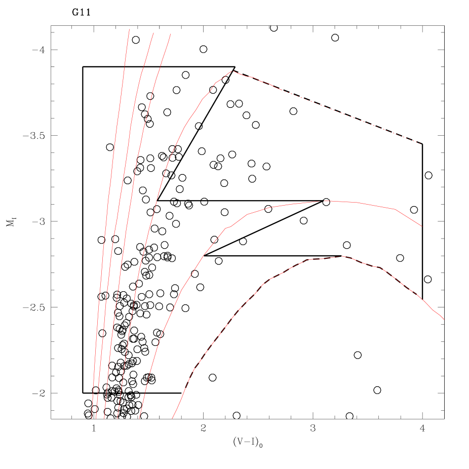
Figure 13: This plot illustrates how our interpolation scheme works. To the left of jagged boundary, we interpolate in color, while to the right, metallicity is determined using an interpolation in magnitude. Stars falling below the curved locus of NGC 6528 are excluded from the sample, but represent only $\approx 1$% of the total in any field.

Figure 17: The metallicity distribution for the field G64 shows the effect of choosing different parameters. The detailed shape of the abundance distribution and the possible existence of a metal poor peak are both sensitive to these choices. Panel (a): Using our adopted CG metallicity scale, distance modulus, and reddening. Panel (b): same as (a), ZW metallicity scale. Panel (c): $(m-M)_{0}$ increased by 0.15 mag, and (d): $(m-M)_{0}$ decreased by 0.15 mag. Panel (e): $E(B-V)$ increased by 0.05 mag, and (f): $E(B-V)$ decreased by 0.05 mag.

Figure 20: Map of the spatial and chemical substructures as described by Ferguson et al. (2002) (their Fig. 7). The positions of our fields are plotted over the cartoon describing the location of the possible projected orbit of the ”giant stellar stream”, the ”northern spur”, and the ”G1 clump”.

Figure 21: Metallicity parameters, derived from the MDs, are plotted versus the angular distance from the center of M31. $\rm[Fe/H]<-1.4$ [Metal-Poor or Young – MP or Y], and $\rm[Fe/H]>-0.2$ [Very Metal-Rich – VMR], versus (a) the X-coordinate, (b) Y, (c) R, the galactocentric distance, respectively. A few fields are evidenced by different symbols (see Sect. 9.2.1): G287 (solid circle); G87 (solid square); G219 (star) and G319 ($\times$).

Figure 22: Panel (a): Fraction of the Metal-Poor Population (with $\rm[Fe/H]<-0.8$ [MPP] plotted versus the absolute distance from the major axis $|Y|$. Panel (b): Median metallicity (GC97-scale) plotted vs. the absolute distance from the major axis $|Y|$.