Type Ia Supernova models: latest developments

Abstract

Supernovae of type Ia (SNe Ia) are very important for cosmography. To exclude systematic effects in linking the observed light of distant SNe Ia to the parameters of cosmological models, one has to understand the nature of supernova outbursts and to build accurate algorithms for predicting their emission.
We review the recent progress of modeling the propagation of nuclear flame subject to numerous hydrodynamic instabilities inherent to the flame front. The Rayleigh–Taylor (RT) instability is the main process governing the corrugation of the front on the largest scales, while on the smallest scales the front propagation is controlled by the Landau-Darrieus instability.
Based on several hydrodynamic explosion models, we predict the broad-band UBVI and bolometric light curves of SNe Ia, using our 1D-hydro code which models multi-group time-dependent non-equilibrium radiative transfer inside SN ejecta. We employ our new corrected treatment for line opacity in the expanding medium, which is important especially in UV and IR bands. The results are compared with the observed light curves. Especially interesting is a recent 3D-deflagration model computed at MPA, Garching, by M. Reinecke et al.

1 Introduction

Supernovae of type Ia (SNe Ia) are important for cosmology due to their brightness. They are not standard candles, but can be used for measuring distances (i.e., for cosmography) with the help of the peak luminosity – decline rate correlation, established by Yu.P. Pskovskii [28] and M.M. Phillips [26] (see the review [22]). The physical understanding of the Pskovskii-Phillips relation is crucial for estimating the validity of cosmological results obtained with SNe. To exclude systematic effects in linking the observed light of distant SNe Ia to the parameters of cosmological models, one has to understand the nature of supernova outbursts and to build accurate algorithms for predicting their emission.

This involves:

• understanding the progenitors of SNe Ia;

• the birth of thermonuclear flame and it accelerated propagation leading to explosion;

• light curve and spectra modeling.

Although there is no doubt that an SN Ia outburst is a result of thermonuclear explosion, the details of the process are not yet clear. We point out some problems which seem most important to us.

We review the recent progress of modeling the propagation of nuclear flame subject to numerous hydrodynamic instabilities inherent to the flame front. The Rayleigh–Taylor (RT) instability is the main process governing the corrugation of the front on the largest scales, while on the smallest scales the front propagation is controlled by the Landau-Darrieus instability.

Based on several hydrodynamic explosion models, we predict the broad-band UBVI and bolometric light curves of SNe Ia, using our 1D-hydro code which models multi-group time-dependent non-equilibrium radiative transfer inside SN ejecta. We employ our new corrected treatment for line opacity in the expanding medium, which is important especially in UV and IR bands. The results are compared with the observed light curves. It seems that classical 1D thermonuclear supernova models produce the light curves that fit the observations not so good as the recent angle-averaged 3D deflagration model computed at MPA, Garching, by M. Reinecke et al.  [29]. We believe that the main feature of the latter model, which allows us to get the correct flux during the first month, is strong mixing that moves the material enriched with radioactive nickel-56 to the outermost layers of the SN ejecta.

2 Progenitors

There is no hope to get a thermonuclear supernova from a normal star composed of a classical plasma. Those stars have negative effective heat capacity and they are thermally stable. The situation changes, if a star is made of a degenerate matter. The total heat capacity becomes positive, and runaway can set in as in terrestrial explosives. So, a progenitor of SN Ia must be a degenerate star - a white dwarf.

A single white dwarf is unable to explode, it cools down. But when it is in a binary system the chances to produce a supernova do appear (we need only one in $\sim 300$ dying white dwarfs to explode in order to explain the rate of SNe Ia). Even if the binary has two dead white dwarfs, it can explode because they can merge due to emission of gravitation waves (double-degenerate, or DD scenario [16]). If one star in the binary is alive, the white dwarf can accrete its lost mass and reach an instability (single-degenerate, or SD scenario [37, 8]). It is unclear which scenario is most important, there are strong arguments [19] from chemical evolution that only SD is the viable one. On the other hand, it seems that DD can produce a richer variety of SN Ia events. Moreover, discoveries of intergalactic SNe Ia [4, 11] can be explained more naturally, because a DD system may evaporate from a galaxy. It is quite likely that both scenarios are being played, but their relative role may change in young and old galaxies. If so, a systematic trend may appear in SNe Ia properties with the age of Universe, and this may have important consequences for cosmology.

3 Thermonuclear flames

After merging in DD scenario, or after the white dwarf accretes large amount of material in SD case, the explosive instability develops. In principle, combustion can propagate either in the form of a supersonic detonation [1] wave, or as a subsonic deflagration [17, 24] (flame). In detonation, the unburned fuel is ignited by a shock front propagating ahead of the burning zone itself. In deflagration, the ignition is governed by heat and active reactant transport, i.e. by thermal conduction and diffusion.

3.1 Laminar flames

Most likely, the runaway starts as a laminar flame propagating due to thermal conduction.

The rate of thermonuclear heating scales as

$$\langle\sigma v_{0}\rangle\sim\exp-(\alpha_{G}/T)^{1/3}$$

due to the Gamow’s peak: the chances to penetrate the Coulomb barrier for fast nuclei grow, but the tail of Maxwell distribution goes down. Here $\alpha_{G}$ depends strongly on nuclei charges $Z_{i}$: $\alpha_{G}\propto Z_{1}^{2}Z_{2}^{2}$, thus high-$Z$ ions can fuse only at high $T$. Small perturbations of $T$ produce huge variations in energy production rate since, normally, $T\ll\alpha_{G}$.

In terrestrial flames, the ‘fusion’ of molecules goes with the rate:

$$\langle\sigma v_{0}\rangle\sim\exp(-{E_{a}/{\mathcal{R}}T}),$$

– the Arrhenius law of chemical burning. Here $E_{a}$ is activation energy. The parameter, showing the strong $T$-dependence of the heating

$$\mathrm{Ze}={\partial\log\langle\sigma v_{0}\rangle/\partial\log T}\simeq{E_{a}/{\mathcal{R}}T}$$

is called the Zeldovich number in the theory of chemical flames. For them typically $\mathrm{Ze}\sim 10\dots 20$. The classical theory [41] predicts the flame speed

$$v_{\mathrm{f}}\approx\mathrm{Ze}^{-1}[{v_{T}l_{T}}/\tau_{\mathrm{reac}}(T_{2})]^{1/2},$$

with $T_{2}$ – the temperature of burnt matter (ashes) and $\tau_{\mathrm{reac}}(T)\propto\exp[E_{a}/({\mathcal{R}}T)]$. In SNe, for nuclear flames, $\tau_{\mathrm{reac}}(T)\propto\exp[\alpha_{G}^{1/3}/(3T^{1/3})]$, and,

$$\mathrm{Ze}={\partial\log\langle\sigma v_{0}\rangle/\partial\log T}\simeq\alpha_{G}^{1/3}/(3T^{1/3}),$$

which has values very similar to terrestrial chemical flames.

A big difference with chemical flames is the ratio of heat conduction and mass diffusion, the Lewis number, $\mathrm{Le}=(v_{T}l_{T})/(v_{D}l_{D})$. $\mathrm{Le}\sim 1$ in laboratory gaseous flames, while $\mathrm{Le}\sim 10^{7}$ in thermonuclear SNe, since heat is transported by relativistic electrons, $v_{T}\sim c$, and there is almost no diffusion, $l_{T}\gg l_{D}$. Nevertheless, the modern computations [36] follow the old theory [41] closely. The conductive flame propagates in a presupernova with $v_{\rm f}$ which is too slow to produce an energetic explosion: the ratio of $v_{\rm f}$ to sound speed, i.e. the Mach number, Ma, is very small (see Table 1). The star has enough time to expand, to cool down, and the burning dies completely. So an acceleration of the flame is necessary in order to explain the SN phenomenon. This is the main problem in current research of SNe Ia hydrodynamics.

Table 1: Flame speed $v_{\mathrm{f}}$ and width $l_{\mathrm{f}}$ in C+O [36]

$\rho$	$v_{\mathrm{f}}$	$l_{\mathrm{f}}$	$\Delta\rho/\rho$	Ma
$10^{9}$ gcc	km/s	cm
6	214	$1.8\times 10^{-5}$	0.10	$2\times 10^{-2}$
1	36	$2.9\times 10^{-4}$	0.19	$4\times 10^{-3}$
0.1	2.3	$2.7\times 10^{-2}$	0.43	$4\times 10^{-4}$

3.2 Flame Instabilities and its Acceleration

There is a rich variety of instabilities that can severely distort the shape of a laminar flame. The Rayleigh–Taylor (RT) instability governs the corrugation of the front on the largest scales. On the smallest scales the flame is controlled by the Landau-Darrieus (LD) instability. RT, LD instabilities and turbulence make computations difficult, but without them a star would not explode. All these instabilities were considered already by L.Landau [21] as a means to accelerate the flame.

Although he did not used a term ‘Rayleigh-Taylor instability’, Landau derived his dispersion relation with account of gravity, so RT is there! Let $k$ be wave number, and $\Omega$ frequency of perturbations on the flame front, the shape of perturbations being of the form $\exp(iky+\Omega t)$. Here we reproduce most important expressions for the Landau dispersion relation when $g\neq 0$ and the surface tension of the fuel is $\alpha$. The notation below follows Landau [21], so $v_{1}$ is the velocity of fuel, $v_{2}$ the same for ashes, $j\equiv\rho_{1}v_{1}=\rho_{2}v_{2}$ is the mass flux across the front. Then the Landau dispersion relation is

$$\Omega^{2}(v_{1}+v_{2})+2\Omega kv_{1}v_{2}+k^{2}v_{1}v_{2}(v_{1}-v_{2})-kg(v_{1}-v_{2})+\alpha k^{3}{v_{1}v_{2}/j}=0.$$

Note that this relation contains RT instability: when $k$ is small and $v_{i}$ is small, we have

$$\Omega^{2}(v_{1}+v_{2})-kg(v_{1}-v_{2})=0.$$

That is, if we replace $v_{i}$ by $1/\rho_{i}$ using $j=\rho_{i}v_{i}=\mathrm{const}$, we get a ‘pure’ RT dispersion equation.

When surface tension is not negligible, we have its stabilizing effect in RT:

$$\Omega^{2}(v_{1}+v_{2})-kg(v_{1}-v_{2})+\alpha k^{3}{v_{1}v_{2}/j}=0.$$

But this is normally important only for very short waves, and if we have

$$kv_{1}v_{2}\gg g\;,$$

i.e. a case of short, but not extremely short waves, then LD becomes important while the term with $\alpha$ can still remain negligible. The latter inequality means that gravity can be ignored, but it is just

$$\frac{1}{k}\ll\ell_{\min}=\frac{v_{1}v_{2}}{g}.$$

A fast flame runs from RT instability away, and the RT instability has no time to develop. But this does not mean that the flame becomes stable! No stabilization is obtained for waves below $\ell_{\min}$, if the role of $\alpha$ or a thermal diffusion is negligible, but the instability looks now not as RT, but as a ‘pure’ LD. Since $\epsilon=v_{1}/v_{2}<1$ (from mass flux $j\equiv\rho_{1}v_{1}=\rho_{2}v_{2}$ and $\rho_{\rm 1}>\rho_{\rm 2}$) this gives a growing mode of LD instability:

$$\Omega_{\mathrm{LD}}=\frac{\sqrt{\epsilon+\epsilon^{2}-\epsilon^{3}}-\epsilon}{\epsilon+1}kv_{2}.$$

Of course, in real life one has to use the full Landau relation, since the subdivision into domains of RT and LD instabilities is only approximate. In many laboratory experiments laminar flames remain stable. Below a certain scale, so-called Markstein length, dissipative effects (like thermal conduction) dominate and smear out all perturbations, so that the flame may remain stable on small scales. In the majority of experiments the flame is attached to a burner, which sets bounds to the development of LD instability at the Markstein scale, but some special experiments with spherical flames do show a growth of LD instability and fractalization of the front. Very nice examples of the action of the LD instability are also observed in growth of bubbles in a overheated liquid.

Because of instabilities, the flame surface becomes wrinkled and its area grows as $S\propto\bar{R}^{\alpha}\;,$ with average radius $\bar{R}$ and $\alpha>2$, i.e. faster than $S\propto\bar{R}^{2}$. In other words the surface becomes ‘fractal’. The exponent $\alpha$ is actually the fractal dimension, $\alpha=D_{\rm F}$. The effective flame speed is determined [39] by the ratio of the maximum scale of the instability to the minimum one: $v_{\rm eff}=v_{\rm f}(\lambda_{\rm max}/\lambda_{\rm min})^{D_{\rm F}-2}.$

Proper understanding of the behavior of flames cannot be reached if we restrict ourselves to a linear analysis of the problem, even if we take into account dissipation. However, good progress can be made with the help of a simple nonlinear model for the flame.

When the vorticity is not important it is possible to study in detail the non-linear stage of LD instability and to find the fractal dimension [5]. Instead of $\epsilon$ we define

$$\eta=\Delta\rho/\rho=1-\rho_{\rm b}/\rho_{\rm u}=1-\epsilon\;.$$

For $\rho_{1}\gtrsim 10^{8}$ g/cm³, which is typical for preSN cores, $\eta\lesssim 0.4$, since the unburned matter is very degenerate and its thermal expansion relatively low. For small $\eta$, it is easy to show that the flow behind the flame front remains irrotational (to first order relative to $\eta$) if the incoming flow is potential and to use a simple model to compute the flame propagation. Laboratory flames in gases have typical values of $\eta\approx 0.8$. In this case a lot of vorticity is generated on the front and the simple model is not applicable.

One can see that for low $\eta$ fractalization is not so pronounced as for high density jumps. We predict [5],

$$D_{\rm F}(\eta)({\rm LD})\rightarrow 1+D_{0}\eta^{2},\;\mbox{ when}\;\eta\rightarrow 0\;.$$

Making a least-square fit to the power law dependence of the length of the flame on the mean radius yields the values in the Table 2. We find that $D_{0}\approx 0.3$.

Table 2: $D_{\rm F}$ for small $\eta=\Delta\rho/\rho$.

$\eta$	$\eta^{2}$	$D_{\rm F}$
0.3	0.09	1.022
0.35	0.122	1.039
0.4	0.16	1.046

3.3 Numerical Thermonuclear Flames

The fractal description is good for LD instability while it remains mild, because it operates in a star on the scales from the flame thickness (a tiny fraction of a cm) up to $\sim 1$ km. For the RT instability, $\lambda_{\rm max}/\lambda_{\rm min}$ is very uncertain and the fractal dimension is uncertain too. (Although a dependence of the flame fractal dimension on the density jump across the front was found in SPH simulations of the flame subject to RT instability [7] similar to the LD case).

So a direct 3D numerical simulation is necessary. The same is true for a low density regime of LD when it is strongly coupled to turbulence (generated on the front, or cascading from large RT vortices). A great progress is achieved here in several groups [14, 29, 31, 18]. When simulating 3D turbulent deflagrations one encounters two problems: the representation of the thin moving surface separating hot and cold material, and the prescription of the local velocity $v_{\mathrm{f}}$ of this surface as a function of the large-scale flow with a crude numerical resolution $>1$ km. One solution is sketched in [29]; for a different approach see [18]. In spite of the progress this problem cannot be treated as completely solved, and even 1D approach may give interesting results, especially for unusual SNe Ia [10].

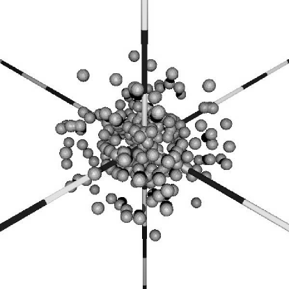
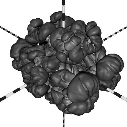
Figure 1: Snapshots of the flame front for 3D simulations [30]. Left panel: initial multi-point ignition. Right panel: flame after 0.5 seconds

4 Light curves of SNe Ia

4.1 Basics

At the moment, there are many models of thermonuclear explosion of a star, that lead to the event we know as SN Ia. Only a few parameters, such as kinetic energy and total ⁵⁶Ni production, can be derived directly from the modelling of the explosion and compared with the observational values. The subsequent evolution of the exploded star gives us much more possibilities to compare models and to decide which one fits observations better by reproducing more details in SN Ia light curves and spectra. We will focus here on the broad-band UBVI and bolometric light curve computations for SN Ia models.

There are several effects in SNe physics which lead to difficulties in the light curve modelling of any type of SNe. For instance, an account should be taken correctly for deposition of gamma photons produced in decays of radioactive isotopes, mostly ⁵⁶Ni and ⁵⁶Co. After being emitted, gamma photons travel through the ejecta and can finish up in either thermalization or in non-coherent scattering processes. To find this one has to solve the transfer equation for gamma photons together with hydrodynamical equations. Full system of equations should involve also radiative transfer equations in the range from soft X-rays to infrared for the expanding medium [6].

There are millions of spectral lines that form SN spectra, and it is not a trivial problem to find a convenient way how to treat them even in the static case. The expansion makes the problem much more difficult to solve: hundreds or even thousands of lines give their input into emission and absorption at each frequency.

On the first glance, the modelling of SNe Ia seems easier than that of other types of supernovae, since the hydro part is very simple: coasting stage starts very early, there are no shocks and no additional heating from them.

Figure 2: The distribution of the ratio of actual radiation energy density to the blackbody one at the local gas temperature inside the ejecta at different times. It demonstrates how radiation is decoupled from matter.

On the other hand, much more difficulties arise in the radiation part. SNe Ia becomes almost transparent in continuum at the age of a few weeks. This means that NLTE effects are stronger than for other types of supernovae. Radiation is decoupled from matter within the entire SN Ia ejecta even before maximum light (which occurs around the 20th day after explosion), see Fig. 2 and also [12]. In this case one cannot ascribe the gas temperature, or any other temperature, to radiation, since SN Ia spectrum differs strongly from a blackbody one. Instead, one has to solve a system of time-dependent transfer equations in many energy groups, with an accurate prescription for treatment of a huge number of spectral lines, which are the main source of opacity in this type of SNe [3, 27].

Recently, powerful codes appear aimed to attack a full 3D time-dependent problem of SN Ia light [15]. Yet there are some basic questions, like averaging the line opacity in expanding media, that remain controversial.

We present theoretical UBVI- and bolometric light curves of SNe Ia for several explosion models, computed with our multi-group radiation hydro code. We employ our new corrected treatment for line opacity in the expanding medium. The results are compared with observed light curves.

4.2 Method

We compute broad-band UBVI and bolometric light curves of SNe Ia with a multi-energy radiation hydro code STELLA. Time-dependent equations for the angular moments of intensity in fixed frequency bins are coupled to Lagrangean hydro equations and solved implicitly [6]. Thus, we have no need to ascribe any temperature to the radiation: the photon energy distribution may be quite arbitrary.

Figure 3: UBVI light curves of the model W7 with two opacity approximations: Eastman–Pinto (dashed) and our new approach (solid). UBV bands remain almost unaffected, while I–band shows now a structure more similar to what one can observe for real SNe Ia, though not identical. Crosses, stars and triangles show the light curves for three observed SNe Ia.

While radiation is nonequilibrium in our approximation, ionization and atomic level populations are assumed to be in LTE. The effect of line opacity is treated as an expansion opacity according to Eastman & Pinto [13] and to our new recipes [33]. We have compared the results and found that infrared bandpass (in which the ejecta are most transparent) is more sensitive to the treatment of opacity than UBV, so one should be very careful on this point. See Fig. 3 for the comparison of SN Ia light curves calculated with these two approaches. To simulate NLTE effects we used the approximation of the absorptive opacity in spectral lines. NLTE results [3] and ETLA approach [27] demonstrate that fully absorptive lines gives us an acceptable approximation of NLTE effects.

We treat gamma-ray opacity as a pure absorptive one, and solve the $\gamma$-ray transfer equation in a one-group approximation following [35]. The heating by decays ⁵⁶Ni $\to$ ⁵⁶Co$\to$ ⁵⁶Fe is taken into account.

In the calculations of SN Ia light curves we use up to 200 frequency bins and up to $\sim 400$ zones as a Lagrangean coordinate.

4.3 Light curves for presupernova models

In our previous analysis we have studied two Chandrasekhar-mass models: the classical deflagration model W7 [25] and the delayed detonation one DD4 [40], as well as two sub-Chandrasekhar-mass models: helium detonation model LA4 [23] and low-mass detonation model WD065 with low ⁵⁶Ni production [32], which was constructed for modelling subluminous SNe Ia events, such as SN 1991bg. All those models were simplified spherically-symmetrical (1D) ones.

Figure 4: UBVI light curves for 4 1D models (W7 – solid line, DD4 – dots, LA4 – dashes, WD065 – dash-dots). Crosses, stars and triangles show the light curves for three observed SNe Ia.

The UBVI light curves of 1D models are shown in Fig. 4. The Chandrasekhar-mass models demonstrate almost identical light curves. The sub-Chandrasekhar-mass ones are more different. WD065 has almost similar element distribution as Chandrasekhar-mass models, and the shape of its light curve is in principle the same as that of W7 and DD4. It is just much dimmer due to an order of magnitude less ⁵⁶Ni abundance.

LA4 is very different from any other model, since the explosion there started on the surface of a white dwarf, not in the center, as for every other model, so there is a ⁵⁶Ni layer near the surface in LA4. This feature explains why the model is essentially bluer than all three others. During first weeks UV quanta are locked inside the models with ⁵⁶Ni in the center and come out only if they are splitted into several redder photons, while in LA4 model they can travel outside from the surface freely. Unfortunately, LA4 seems much bluer than real SNe Ia, its rise and decline rates are also too fast, so centrally ignited models look better from the observational point of view.

Table 3: Parameters of SN Ia models

Model	DD4	W7	LA4	WD065	MR
$M_{\rm WD}{}^{\rm a}$	1.3861	1.3775	0.8678	0.6500	1.4
$M_{{}^{56}{\rm Ni}}{}^{\rm a}$	0.63	0.60	0.47	0.05	0.42
$E_{51}{}^{\rm b}$	1.23	1.20	1.15	0.56	0.46
ain $M_{\odot}$
bin $10^{51}$ ergs s-1

Recently, an interesting and much more sophisticated 3D deflagration model by M.Reinecke et al. [29] (MR, hereafter) has appeared. Working in more dimensions the authors have to involve less free parameters than was needed in 1D simulations, so they get their model almost from the “first principles”. The main features of the 3D model are compared with the ones of classical 1D models in the Table 3.

Figure 5: UBVI light curves for the 3D (MR; solid) and 1D (W7; dashed) models. Crosses, stars and triangles show the light curves for three observed SNe Ia.

Figure 6: Element distributions for DD4 (top left) W7 (bottom left) and MR (right) models.

From the first glance it seems that the light curves for the models which differ so much could not be similar. Nevertheless, Fig. 5 demonstrates that they are similar in many details. The possible reasons for this can be understood if one has a look at the element distribution over the ejecta. The compositions for W7 and MR models are shown in Fig. 6.

At the moment of our light curve computation the full nuclide yields for MR were not yet obtained. Therefore, the model consisted of the elements, which were chosen as representative examples for the energy release calculation, namely, “Fe” for iron group elements that were divided onto 80% of ⁵⁶Ni and 20% of ⁵⁶Fe, “Mg” for intermediate mass elements, and unburned C and O in equal proportion.

The instabilities that have developed in the 3D model were not supposed to be so huge in approximate 1D models of explosion. This has led to the differences in the nickel distribution over the ejecta: it is mixed to the outermost layers in the 3D model. These layers become much more opaque than in the 1D models, and, despite having less than a half of kinetic energy, the 3D model has a photospheric velocity comparable to that in the 1D models. It is probably still a bit too low, so the light curve is wider, since the ejecta expand a bit slower, and photons are locked inside them for a bit longer time. The broad-band light curves for MR model fit the observations of one of the typical SN Ia, SN 1994D, in $U$ and $B$ bands surprisingly well, while classical 1D models, such as W7 and DD4, show faster decline in the optics than it is observed.

Figure 7: Total (thin dotted) and UVOIR (thick solid) bolometric luminosities of MR (left panel) and W7 (right panel) models compared with observations [9].

Unfortunately, the bolometric light curve for MR model (Fig. 7) is somewhat too slow. The ejecta must expand with higher speed to let photons to diffuse out faster. This means that the total energy must be larger to fit the bolometric observations. The bolometric light curve of W7 is also shown in the Fig. 7. It demonstrate much more acceptable decline rate, though the behaviour of the light curve before maximum light seems better in MR model.

The model MR is not final. The work on getting a new, more energetic 3D model is in progress at the MPA supernova group. It seems that such a model should still be as much mixed as MR. Then one could expect that it would fit the observations of SN Ia bolometric light curves as well as the broad band ones.

There is also another reason which allows us to believe that the MR model is better than the classical 1D models. We calculated in details the X-ray emission of Tycho SNR, which is believed to be the remnant of SN Ia. The code we use takes into account the time-dependent ionization and recombination. We have compared the computed X-ray spectra and images in narrow filter bands with XMM-Newton observations of the Tycho. Our preliminary results [20] show that all Chandrasekhar-mass models produce similar X-ray spectra at the age of Tycho, but they differ strongly in the predictions of how the remnant should look like in the lines of different ions due to very different distribution of elements in the ejecta for 1D and 3D models. We found that W7 and DD4 models produce rather wide ring in Fe lines, while it is narrow for MR model. The image for the latter model is very similar to what is observed.

We believe that the main feature of this model which allows us to get correct radiation during the first month, as well as after a few hundred years, when an SNR forms, is strong mixing that pushes material enriched in iron and nickel to the outermost layers of SN ejecta.

5 Conclusions

There are many points which require attention in research of SNe Ia: progenitors; burning regimes (that may change with the age of Universe [34]). The physical understanding of the Pskovskii-Phillips is not yet achieved (probably it will be reached when the burning will be modeled completely from the first principles, because too many parameters enter in light curve computations).

The new 3D SN Ia model MR [29] is very appealing. Yet it is not a final one: a detailed post-processing of nucleosynthesis changes the composition. It has been done very recently [38], and it is not yet checked in the light curve calculation. Our light curve computations are also preliminary, since more work is needed on the expansion opacity. Hopefully, none of the required improvements will spoil the light curve of this model and its X-ray spectra on the SNR stage, since the specific qualities of the model can be primarily explained by the enrichment of the outermost layers of SN ejecta by Fe and Ni.

The SN light curve modelling still has a lot of physics to be added, such as a 3D time-dependent radiative transfer, including as much as possible of NLTE effects, which are especially essential for SNe Ia [15]. All this will improve our understanding of thermonuclear supernovae.

Acknowledgements

The authors are grateful to Wolfgang Hillebrandt and to Stan Woosley for their hospitality at MPA and UCSC, respectively, and to Bruno Leibundgut for providing us with the data [9] in electronic form. The work is supported in Russia by RFBR grant 02-02-16500, in the US, by NASA grant NAG5-8128 and in Germany, by MPA visitor program.

References

- [1] W.D. Arnett, Ap.Sp.Sci. 5, 180 (1969).
- [2] W.D. Arnett, ApJ 253, 785 (1982)
- [3] E. Baron, P.H. Hauschildt, A. Mezzacappa, MNRAS 278 763 (1996)
- [4] O. Bartunov, Outlying Supernovae - Myth or Reality? UCSB Workshop on SNe, http://www.sai.msu.su/megera/sn/outsn/ (1997).
- [5] S.I. Blinnikov, P.V. Sasorov, Phys.Rev. E53 4827 (1996).
- [6] S.I. Blinnikov et al., ApJ 496, 454 (1998).
- [7] E. Bravo, D.García-Senz, ApJ 450, L17 (1995).
- [8] A. Bragaglia et al., ApJL 365, L13 (1990).
- [9] G. Contardo, B. Leibundgut, W. D. Vacca, A&A 359, 876 (2000).
- [10] N.V. Dunina-Barkovskaya et al., Astron.Letters 27, 353 (2001).
- [11] A.Gal-Yam et al., astro-ph/0211334 (2002).
- [12] R.G. Eastman, In: Thermonuclear Supernovae. ed. by P. Ruis-Lapuente et al. (Kluwer Academic Pub., Dordrecht, 1997) p. 571.
- [13] R.G. Eastman, P.A. Pinto, ApJ 412, 731 (1993)
- [14] W. Hillebrandt, J. C.Niemeyer, Ann. Rev. Astron. Ap. 38, 191 (2000).
- [15] P. Höflich, Workshop on Stellar Atmosphere Modeling, 8-12 April 2002 Tuebingen. Eds: I. Hubeny, D. Mihalas, K. Werner, astro-ph/0207103 (2002).
- [16] I.J. Iben, et al., ApJ 475, 291 (1997).
- [17] Ivanova L.N. et al., Space Sci. 31, 497 (1974).
- [18] A. Khokhlov, e-print astro-ph/0008463 (2000).
- [19] C. Kobayashi et al., ApJL 503, L155 (1998).
- [20] D.I. Kosenko, E.I. Sorokina, S.I. Blinnikov, P. Lundqvist, K.A. Postnov, Submitted to 34th COSPAR Sci. Assembly, Houston, 10-19 october 2002 (astro-ph/0212188).
- [21] L.D. Landau, Acta Physicochim. USSR 19, 77 (1944)
- [22] B. Leibundgut: Astr.Ap.Rev. 10, 179 (2000).
- [23] E. Livne, D. Arnett, ApJ 452, 62 (1995)
- [24] K. Nomoto et al., Ap.Space Sci. 39, L37 (1976).
- [25] K. Nomoto, F.-K.Thielemann, K. Yokoi, ApJ 286, 644 (1984)
- [26] M.M. Phillips, ApJL 413, L105 (1993)
- [27] P.A. Pinto, R.G. Eastman, ApJ 530, 757 (2000)
- [28] Yu.P. Pskovskii, Astron. Zh. 54, 1188 (1977)
- [29] M. Reinecke, W. Hillebrandt, J. C. Niemeyer, A&A 386, 936 (2002)
- [30] M. Reinecke: private communication (2002)
- [31] F.K. Röpke et al., Proc. 11th Workshop Nuclear Astrophysics, rmany, February 11-16, 2002, W.Hillebrandt and E. Müller (Eds.). MPA/P13 (2002), p. 41 (astro-ph/0204036).
- [32] P. Ruiz-Lapuente et al., Nature 365,728 (1993)
- [33] E.I. Sorokina, S.I. Blinnikov: Nuclear Astrophysics, 11th Workshop at Ringberg Castle, Tegernsee, Germany, February 11–16, 2002, ed. by E. Müller, W. Hillebrandt, pp. 57–62 (astro-ph/0212187)
- [34] E.I. Sorokina, S.I. Blinnikov, O.S. Bartunov, Astron. Letters 26, 67 (2000) S.I. Blinnikov, E.I. Sorokina: A&A 356, L30–L32 (2000)
- [35] D.A. Swartz, P.G. Sutherland, R.P. Harkness, ApJ 446, 766 (1995)
- [36] F.X. Timmes, S.E. Woosley, ApJ 396, 649 (1992).
- [37] J. Whelan, I. J. Iben, ApJ 186, 1007 (1973).
- [38] C. Travaglio, private communication (2002)
- [39] S.E. Woosley, in: Supernovae, ed. A. G. Petschek, A & A library, 1990, p. 182
- [40] S.E. Woosley, T.A. Weaver. In: Supernovae, ed. by J. Audouze et al., Elsevier Science Publishers, Amsterdam (1994), p.63
- [41] Ya.B. Zeldovich, D.A. Frank-Kamenetsky, Acta Physicochim. USSR 9, 341 (1938)