000 \Year0000 \Month00 \Pagespan000000 \lhead[0]A.N. H. Eerik, P. Tenjes: Metallicity distribution of GCSs \rhead[Astron. Nachr./AN 3XX (2002) X]0 \headnoteAstron. Nachr./AN 3XX (2002) X, XXX–XXX
Metallicity distributions of globular cluster systems in galaxies
Abstract
We collected a sample of 100 galaxies for which different observers have determined colour indices of globular cluster candidates. The sample includes representatives of galaxies of various morphological types and different luminosities. Colour indices (in most cases , but also and ) were transformed into metallicities according to a relation by Kissler-Patig (1998). These data were analysed with the KMM software in order to estimate similarity of the distribution with uni- or bimodal Gaussian distribution. We found that 45 of 100 systems have bimodal metallicity distributions. Mean metallicity of the metal-poor component for these galaxies is of the metal-rich component . Dispersions of the distributions are 0.15 and 0.18, respectively. Distribution of unimodal metallicities is rather wide. These data will be analysed in a subsequent paper in order to find correlations with parameters of galaxies and galactic environment.
keywords:
galaxies: halos – galaxies: star clusters – galaxies: abundances – globular clusters: generalptenjes@ut.ee
1 Introduction
In galaxy formation theories different physical processes may determine the formation and evolution of galaxies with different luminosities and different morphological types. Star formation is regulated by hierarchical clustering of dark matter halos, accretion of gas into dark matter potential well, reionisation of ISM by first stars, outflows of gas, galactic mergers, etc. On the other hand, despite varieties between galaxies it is important to find similarities between them. Globular cluster systems (GCSs) are known to exist in galaxies with rather different morphology (see e.g. Ashman & Zepf 1998). Therefore, it is interesting to compare the properties of GCSs in galaxies with different morphological types and different luminosities.
It has been firmly established that GCSs of many galaxies may have bimodal metallicity distribution (e.g. Ashman & Zepf 1998; Gebhart & Kissler-Patig 1999), and different scenarios have been proposed to explain bimodality. It is rather reasonable that mergers between galaxies may stimulate the formation of globular clusters (GCs) as well as dwarf galaxies (Schweizer 1987; Ashman & Zepf 1992; Weilbacher et al. 2000), but before accepting mergers as a dominating mechanism in creating bimodality, additional studies and arguments are needed. A multi-phase collapse process (Forbes et al. 1997) as a dominating mechanism needs additional theoretical calculations based on the general theory of the reionisation epoch in galactic formation. Accretion of metal-poor GCs from dwarf galaxies (Côté et al. 1998) is also a rather plausible process, but before accepting it as a dominating process, additional studies are needed. Although the reasons of uni- or bimodality have not been fully understood, serious attempts have been made to explain bimodality in the case of some particular galaxies or particular group of galaxies (e.g. van den Bergh 1998; Harris et al. 2000; Forbes et al. 2001; Larsen et al. 2001a; Ashman & Zepf 2001).
In this paper, we compile a sample of colour distributions of GCS in galaxies. Colours were corrected from absorption in our Galaxy according to Schlegel et al. (1998) if not mentioned otherwise. Colours were analysed with the help of the KMM algorithm (Ashman, Bird & Zepf 1994). As initial data for the KMM we used individual cluster data and not the histograms of metallicity distributions. The KMM algorithm allows to determine the maxima in uni- or bimodal metallicity distributions. Correlations of derived metallicities with various properties of host galaxies and spatial distribution parameters of GCSs will be studied in a subsequent paper.
2 Sample and metallicity calibration
Colour distributions are now available for GCSs in nearly 110 galaxies. However, in some galaxies the observed number of clusters is too small for statistical analysis. After rejecting these systems, our sample includes GCSs in 100 galaxies. This sample contains representatives of host galaxies of different morphological types and different luminosities. Tables 1 and 2 present the names, morphological types, absolute luminosities in V colour, estimated total numbers of globular clusters and references to the sources of globular cluster data.
| Galactic | Morph. | Source | ||
|---|---|---|---|---|
| NGC name | type | |||
| 224 | Sb | -21.8 | 2 | |
| 474 | S0 | -21.4 | 1 | |
| 524 | S0 | -22.1 | 2 | |
| 584 | E4 | -21.4 | 3 | |
| 596 | Ep | -20.9 | ||
| 598 | Scd | -19.2 | 15 | |
| 821 | E4/6 | -20.8 | 3 | |
| 1023 | S0 | -21.0 | ||
| 1052 | E4 | -20.9 | 2 | |
| 1199 | E3 | -22.0 | ||
| 1201 | S0 | -20.8 | 1 | |
| 1332 | S0 | -21.2 | 1 | |
| 1374 | E1 | -19.8 | 3 | |
| 1379 | E0 | -19.9 | 3 | |
| 1380 | S0 | -21.7 | 3 | |
| 1387 | S0 | -20.2 | 3 | |
| 1389 | S0 | -19.5 | 1 | |
| 1399 | cD/E1 | -21.8 | 4 | |
| 1400 | S0 | -20.6 | 3 | |
| 1404 | E1 | -21.4 | 3 | |
| 1426 | E4 | -20.4 | ||
| 1427 | E5/3 | -20.4 | 3, 14 | |
| 1439 | E1 | -20.4 | 3 | |
| 1553 | S0 | -21.2 | 3 | |
| 1700 | E4 | -22.2 | 5 | |
| 2300 | S0 | -20.8 | ||
| 2434 | E0 | -20.6 | ||
| 2768 | S0 | -21.9 | 1 | |
| 2778 | E2 | -19.4 | ||
| 2902 | S0 | -20.2 | 1 | |
| 3031 | Sab | -21.1 | 2 | |
| 3056 | S0 | -18.9 | 1 | |
| 3115 | S0 | -20.8 | 3 | |
| 3311 | cD/E0 | -22.3 | 3 | |
| 3377 | E5/6 | -19.9 | 2 | |
| 3379 | E1 | -20.7 | 2 | |
| 3384 | S0 | -20.1 | 2 | |
| 3414 | S0p | -21.0 | 1 | |
| 3489 | S0 | -19.6 | 1 | |
| 3585 | E7 | -21.7 | ||
| 3599 | S0 | -18.4 | 1 | |
| 3607 | S0 | -20.7 | 3 | |
| 3608 | E2 | -20.7 | 2 | |
| 3610 | E5 | -21.5 | 2 | |
| 3640 | E3 | -21.8 | ||
| 3923 | E3/4 | -22.1 | 3 | |
| 4125 | E6p | -22.1 | ||
| 4192 | Sab | -20.7 | ||
| 4203 | S0 | -20.2 | 1 | |
| 4278 | E1/2 | -19.8 | 2 | |
| 4291 | E2 | -20.7 | 2 | |
| 4343 | Sb | -18.8 | ||
| 4365 | E3 | -21.8 | 3 | |
| 4374 | E1 | -21.7 | 3 | |
| 4379 | S0p | -19.6 | 1 | |
| 4406 | E3/S0 | -21.8 | 3 | |
| 4450 | Sab | -22.3 | ||
| 4458 | E0/1 | -19.5 | 6 | |
| 4459 | S0 | -20.9 | 1 | |
| 4472 | E2 | -22.6 | 2 |
| Galactic | Morph. | Source | ||
|---|---|---|---|---|
| name | type | |||
| 4473 | E5 | -20.9 | 6 | |
| 4478 | E2 | -19.9 | ||
| 4486 | cD/E0 | -22.4 | 2 | |
| 4486B | cE0 | -17.8 | 6 | |
| 4494 | E1/2 | -21.0 | 2 | |
| 4526 | S0 | -21.4 | 2 | |
| 4536 | Sbc | -21.7 | ||
| 4550 | S0 | -19.5 | 6 | |
| 4552 | E0/5 | -21.2 | 3 | |
| 4565 | Sb | -21.4 | 7 | |
| 4569 | Sab | -21.8 | 2 | |
| 4589 | E2 | -21.2 | 6 | |
| 4594 | Sa | -22.2 | 12 | |
| 4621 | E5 | -21.3 | 2 | |
| 4649 | E2 | -22.3 | 3 | |
| 4660 | E6 | -19.2 | 6 | |
| 4874 | cD/E0 | -23.1 | 8 | |
| 4881 | E0 | -21.6 | 2 | |
| 4889 | E5/4 | -23.5 | 2 | |
| 5018 | E3 | -22.6 | 4 | |
| 5061 | E0 | -21.6 | ||
| 5128 | E0p | -22.0 | 3 | |
| 5322 | E3/4 | -22.1 | 6 | |
| 5813 | E1/2 | -21.6 | 2 | |
| 5845 | E | -19.3 | 6 | |
| 5846 | E0 | -22.1 | 3 | |
| 5907 | Sc | -21.2 | 7 | |
| 5982 | E3 | -21.8 | 6 | |
| 6702 | E3 | -21.9 | 9 | |
| 6703 | S0 | -21.8 | 1 | |
| 6861 | S0 | -21.8 | ||
| 6868 | E | -22.1 | 13 | |
| 7192 | S0 | -21.5 | ||
| 7332 | E2 | -20.1 | ||
| 7457 | E/S0 | -19.5 | 10 | |
| 7619 | E2 | -22.1 | ||
| 7626 | E1p | -21.9 | 6 | |
| IC1459 | E3 | -21.4 | 6 | |
| IC4051 | E2 | -21.9 | 11 | |
| MW | Sbc | -21.3 | 2 |
Sources for total number of GCs: 1 – Kundu & Whitmore (2001b); 2 – Ashman & Zepf (1998); 3 – Kissler-Patig (1997); 4 – van den Bergh (1998); 5 – Brown et al. (2000); 6 – Kundu & Whitmore (2001a); 7 – Kissler-Patig et al. (1999); 8 – Harris et al. (2000); 9 – Georgakakis et al. (2001); 10 – Chapeton et al. (1999); 11 – Woodworth & Harris (2000); 12 – Larsen et al. (2001b); 13 – Da Rocha et al. (2002), 14 – Forte et al. (2001), 15 – Chandar et al. 2001.
Although the most frequent morphological type is elliptical, the sample includes also spirals from Sa to Sc. Luminosities differ as much as 2 orders of magnitudes.
References to color measurements of globular clusters used in present study are given in Tables 3 and 4. When for a particular galaxy colors are determined by different studies we preferred HST observations to ground based observations and later observations to earlier observations.
The next step is to move from broadband colours to metallicities. This must be done carefully as many calibrations are crude and small uncertainties in GC colours may cause large errors in derived metallicities. Calibration uncertainties are in most cases due to an inadequate database for calibrating any colour indices for metallicities above solar abundance. Nearly all the most often used empirical relations have been derived from colours of Galactic GCs. Due to the fact that the bulk of Galactic GCs are rather blue, these relations hold well only in the range of metallicities Extrapolating these relations to higher values of metallicity, they may not describe reality sufficiently well.
The relationship between the colours , , etc., and metallicities of GCs is usually approximated as linear (see e.g. Couture et al. 1990a,b; Reed et al. 1994; Harris 1996; Kundu & Whitmore 1998; Barmby et al. 2000). For the reason explained above, most of these relations overestimate the metallicity of red clusters. The metallicities of blue clusters are less affected by the choice of the transition relation (different relations give a discrepancy dex in metallicities of blue clusters, for red clusters it is dex). Theoretical models (e.g. Worthey 1994) attribute nonlinear behaviour to the relation between colours and metallicities, i.e. to higher metallicity values (red colours) corresponds a relation with a shallower slope than for blue colours. The relation varies also with the average age of GCS (Schulz et al. 2002).
With the help of more metal-rich GCs in NGC 1399 a good conversion from colour to super-solar metallicities has been derived by Kissler-Patig et al. (1998)
| (1) |
Although this relation is also linear, it is a good compromise to characterize nonlinearity of the theoretical model prediction. Investigation of calibrations that are available for other colours shows that also the relation vs from Geisler & Forte (1991)
| (2) |
offers reliable results.
Analyses of GC metallicities have often been made using the same photometric filters to avoid systematic effects in the conversion to a homogeneous system. Today the situation is even more favourable for large sample statistics. The bulk of the recent GC colours available in literature come from the HST studies and often use the and filters (e.g. Kundu & Whitmore 2001a,b; Larsen et al. 2001a). Many giant galaxies are thoroughly re-investigated in . Therefore, it is possible to compile a homogeneous sample of systems with and colour distributions. From observations in other colour systems only GCSs in NGC 1316 and NGC 1404 are included in the analysis.
Forbes & Forte (2001) have confirmed the relations vs other colours based on Galactic GCs. They show that those relations are applicable for the GCs of early type galaxies using an extrapolation to redder colours. For NGC 1316 and NGC 1404 GCs we use first the following relation from Forbes & Forte (2001)
| (3) |
This relation allows to estimate with an accuracy of . Using expression (1), we convert the derived colours to .
3 Results: globular cluster metallicity distributions
In our study we use for Galactic reddening corrected colour data. Using relations (1) – (3) the derived GC metallicity distributions are tested for bimodality.
In principle, it is possible to determine the bimodality also from a classical histogram. However, in this study we use the KMM algorithm and unbinned GC list to explore bimodality. The KMM test (Ashman, Bird & Zepf 1994) provides a statistical test for comparing the likelihood of the underlying distribution being a single or a double Gaussian. The KMM test also determines the peak values (i.e. mean metallicities) of each subpopulation. The peaks can be determined with an accuracy of 0.05 dex. Homoscedastic fitting mode was used, forcing identical dispersions. Only for galaxies NGC 1399 and NGC 5846 it has been determined that red GCs have a colour distribution almost twice as broad as the blue ones.
The input of the KMM algorithm includes individual data-points, the number of Gaussian components to be fitted and the starting point for the components’ peak values and dispersions.
Because there does not exist general databasis for globular cluster colors in external galaxies we give in Tables 3 and 4 references only to original papers. For galaxies NGC 598, 1380, 1399, 3031, 4472, 4486, 4565, 4594, 5128, 5846 and 7457 data are taken from tables or figures of corresponding original papers. For galaxies NGC 1374, 1379 and 1387 data are taken from electronic database (www.eso.org/ mkissler/Archive). For galaxies NGC 596, 821, 1404, 1426, 1700,2300, 2434, 2788, 3115, 3311, 3585, 3608, 3640, 3923, 4125, 4379, 4406, 4458, 4478, 4621 and 7192 the data are communicated by authors of corresponding papers as personal communication.
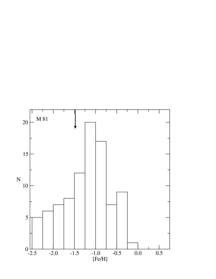
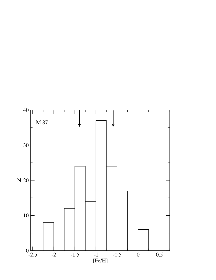
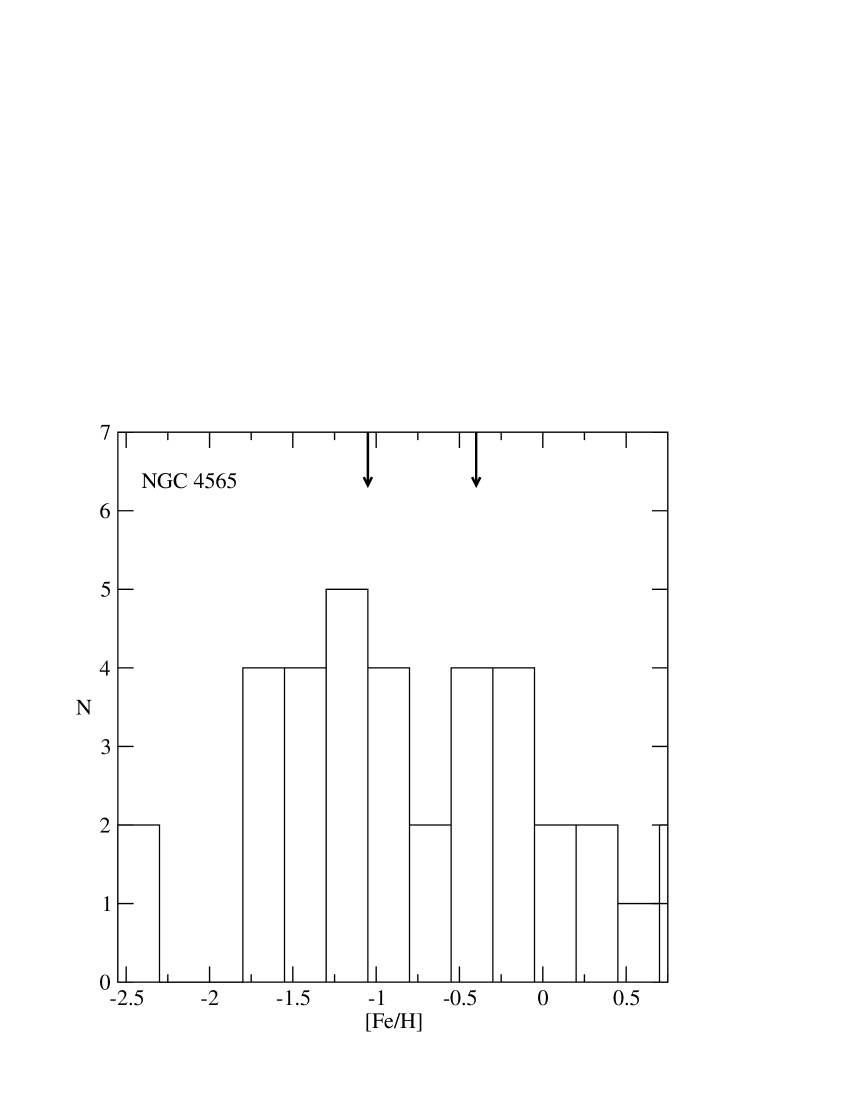
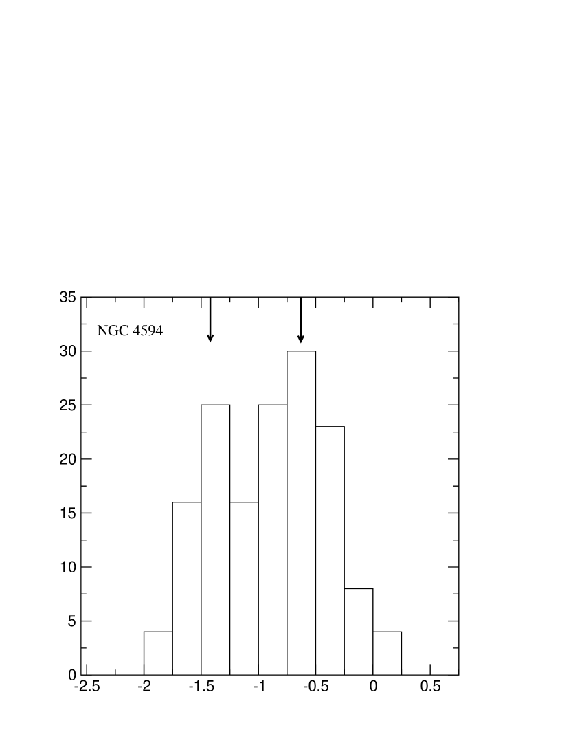
Since KMM is sensitive to highly deviating metallicity values in the data set, only the objects that are within the range are considered. The KMM test also allows to detect bimodality when the metallicity distributions do not visually express several peaks. In Figs. 1 – 4 some characteristic examples of GCSs are given. Arrow(s) at the top of the figures indicate the position of the central values of Gaussian(s). In Table 3, mean metallicities for two Gaussian components are given for galaxies where the KMM test indicated bimodality. In the Table the column labeled “Refer.” refers to the authors of GC colour measurements in a particular galaxy. If the KMM test was done by these authors and the methods correspond to ours, we did not reanalyse the corresponding data and simply accepted metallicity peak values. These cases are designated in the column “Source” by references to corresponding authors. An asterisk in the column “Source” means that the data for a particular galaxy were reanalysed by us. In Table 4 mean metallicities for a single Gaussian component are given for galaxies where the KMM test discovered unimodality.
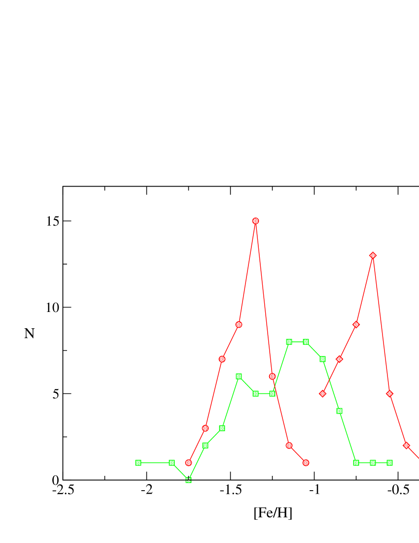
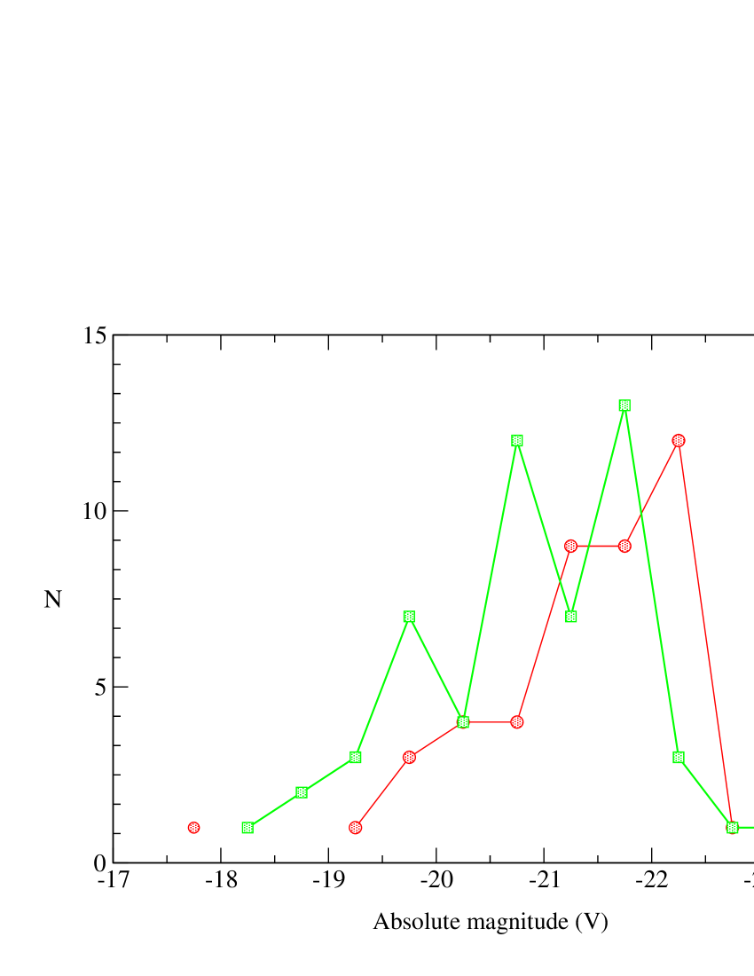
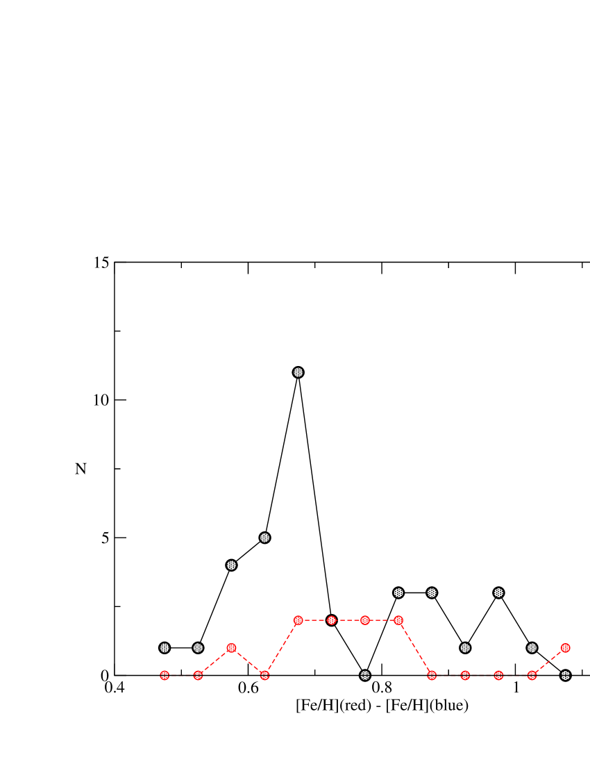
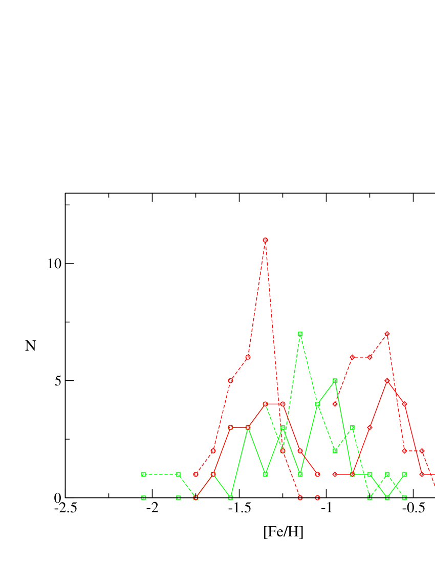
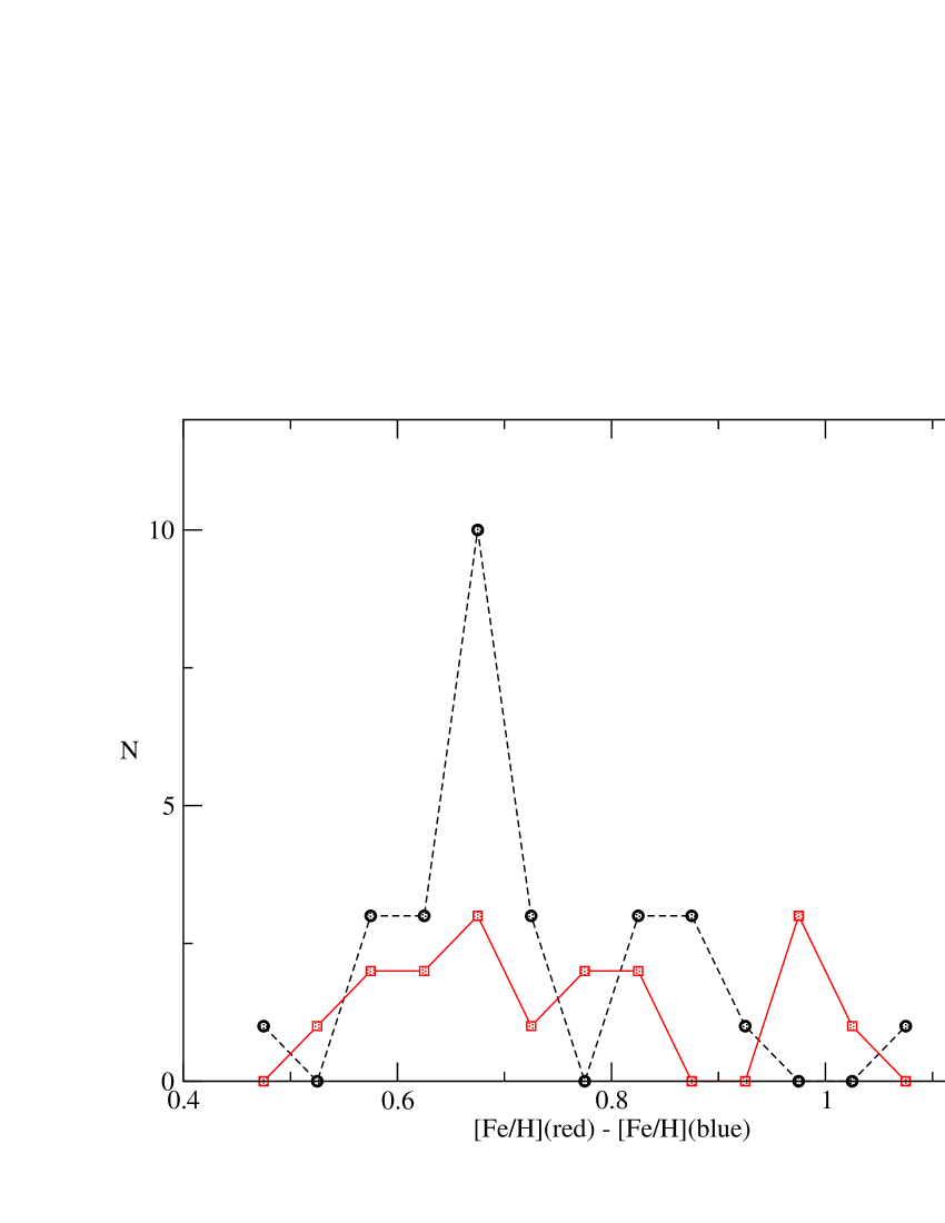
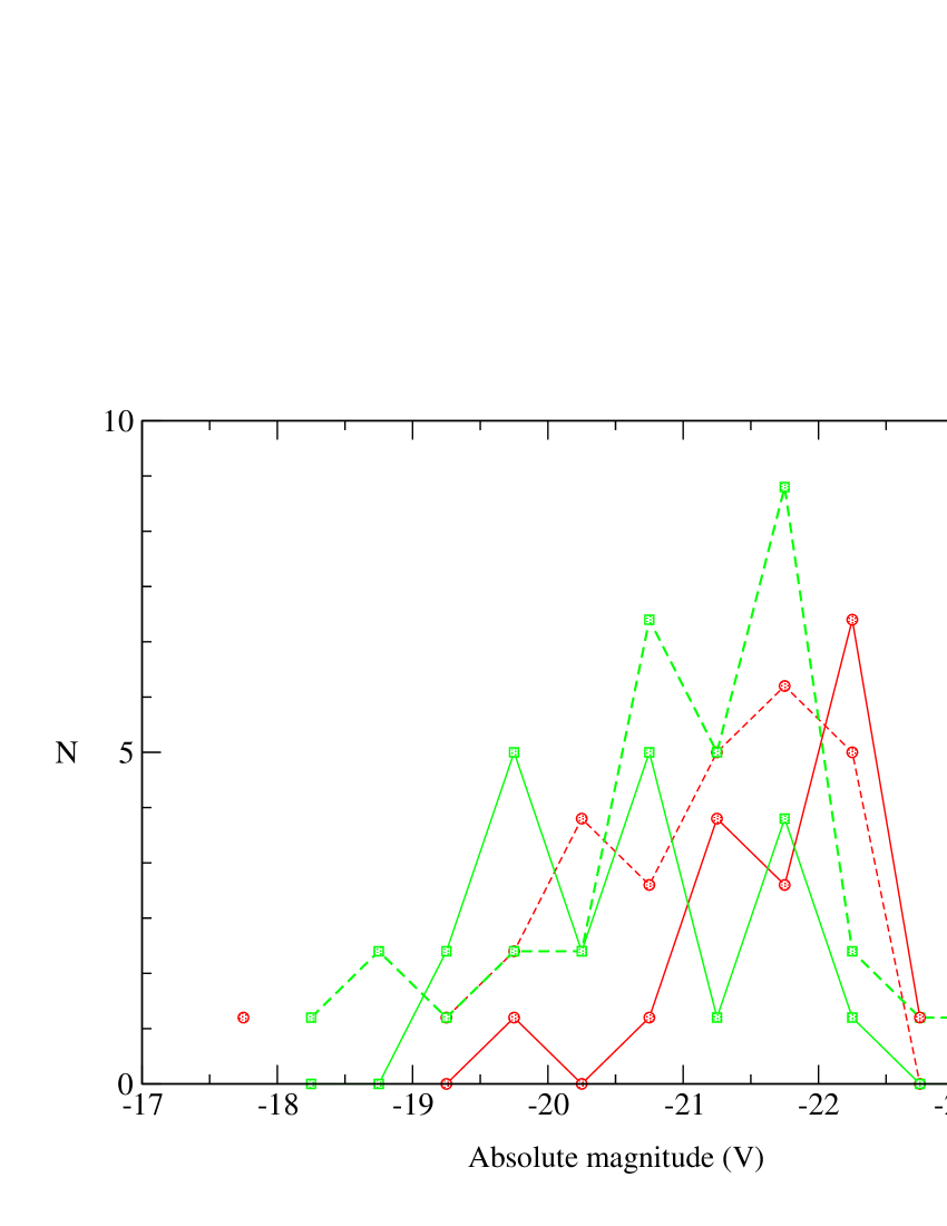
Figure 5 presents the distribution of metallicities from Tables 3 and 4. Mean metallicity of the metal-poor component is the standard deviation of the distribution is 0.15. Mean metallicity of the metal-rich component is the standard deviation is 0.18. Both distributions have similar dispersions and slight asymmetry. Distribution of unimodal metallicities is rather wide. Distribution of metallicity differences between metal-rich and metal-poor peaks in galaxies is given in Fig. 6. Mean difference is the standard deviation is 0.14. Distribution is asymmetric (skewness ), thus the median is perhaps better characteristic of the distribution than the mean. Although the decrease of at small values may be caused by intrinsic characteristics of the KMM test (smaller differences fuse into unimodal distribution) a steep decrease of at higher values seems to be a real property of GCSs. In Fig. 7, we give the luminosity distributions of galaxies with bimodal and unimodal metallicity distributions. In general, luminosity distributions have similar dispersions and skewnesses, but the galaxies with unimodal metallicity distribution are systematically fainter by about mag.
To understand possible systematic biases in further analysis due to the used database, we have repeated Figs. 5-6 separately for GCSs, metallicities of which were determined on the basis of (V–I) and (B–I) colors. color is used only in the case of a few galaxies and it is not possible to study corresponding distributions. Results are presented in Figs. 8-9. Although the number of (B–I) color measurements is rather small for accurate statistics (10 bimodal systems and only 3 unimodal systems), inspection of the figures indicates that metallicities determined from (B–I) colors are slightly shifted in the direction of smaller metallicities. This may raise a question about the precision of color-metallicity calibration. However, the (B–I) sample is small and thus statistical fluctuations are large. There seems to be no systematic shift between the distribution of differences of red (metal-rich) and blue (metal-poor) peaks for GCS with bimodal metallicity distribution.
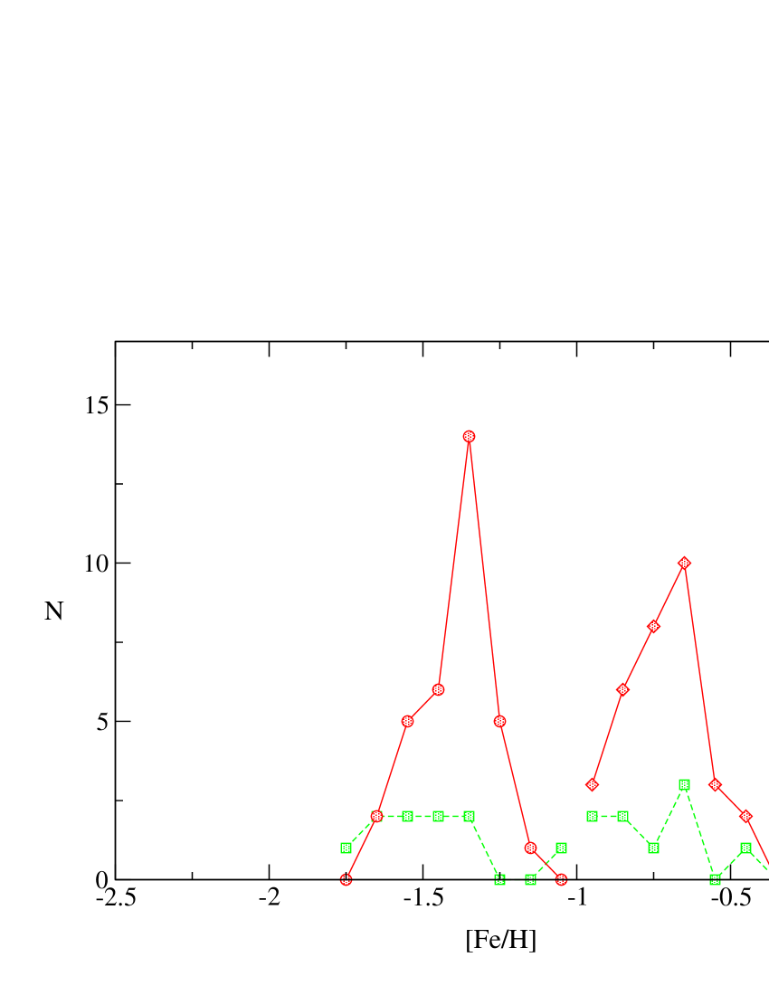
Next, we compare the metallicities of GCSs derived in the present study to those by other authors. We would like to stress that the metallicities are in both cases determined with help of the KMM test. In Figs. 10-12 we repeate Figs. 5-7 but separately for two samples. Solid lines correspond to the sample of GCSs, metallicities of which are determined in the present study, dashed lines correspond to the sample of other papers. We think that there are no systematic differences between the two samples.
| Galaxy | Refer. | Source | ||
|---|---|---|---|---|
| 224 | 22 | -1.43 | -0.60 | 22 |
| 524 | 1 | -1.30 | -0.61 | 1 |
| 584 | 2 | -1.30 | -0.70 | 2 |
| 1023 | 3 | -1.46 | -0.61 | 3 |
| 1052 | 4 | -1.56 | -0.97 | 4 |
| 1199 | 8 | -1.49 | -0.84 | 8 |
| 1380 | 5 | -1.66 | -0.71 | * |
| 1399 | 23 | -1.22 | -0.30 | * |
| 1404 | 6 | -1.45 | -0.67 | * |
| 1427 | 7 | -1.33 | -0.67 | 7 |
| 1439 | 8 | -1.33 | -0.71 | 8 |
| 1700 | 9 | -1.56 | -0.84 | * |
| 2768 | 8 | -1.52 | -0.87 | 8 |
| 3115 | 1 | -1.36 | -0.67 | * |
| 3311 | 10 | -1.52 | -0.94 | * |
| 3377 | 8 | -1.36 | -0.80 | 8 |
| 3379 | 1 | -1.36 | -0.67 | 1 |
| 3384 | 1 | -1.43 | -0.54 | 1 |
| 3923 | 11 | -1.23 | -0.58 | * |
| 4278 | 8 | -1.46 | -0.80 | 8 |
| 4365 | 1 | -1.29 | -0.63 | 1 |
| 4406 | 1 | -1.28 | -0.76 | * |
| 4472 | 12 | -1.10 | -0.50 | * |
| 4473 | 1 | -1.44 | -0.72 | 1 |
| 4478 | 13 | -1.26 | -0.28 | * |
| 4486B | 2 | -1.52 | -0.90 | 2 |
| 4486 | 14 | -1.39 | -0.59 | * |
| 4494 | 1 | -1.55 | -0.89 | 1 |
| 4526 | 2 | -1.62 | -0.74 | 2 |
| 4552 | 1 | -1.39 | -0.67 | 1 |
| 4565 | 15 | -1.05 | -0.40 | * |
| 4594 | 16 | -1.42 | -0.63 | * |
| 4621 | 13 | -1.30 | -0.71 | * |
| 4649 | 1 | -1.38 | -0.56 | 1 |
| 4660 | 13 | -1.46 | -0.97 | 13 |
| 5128 | 17 | -1.11 | -0.16 | * |
| 5846 | 18 | -1.36 | -0.67 | * |
| 5982 | 19 | -1.30 | -0.65 | 19 |
| 6702 | 20 | -1.79 | -0.71 | 20 |
| 6868 | 8 | -1.52 | -0.84 | 8 |
| 7332 | 8 | -1.62 | -0.97 | 8 |
| 7619 | 8 | -1.29 | -0.45 | 8 |
| IC1459 | 19 | -1.30 | -0.48 | 19 |
| IC4051 | 21 | -1.30 | -0.71 | 21 |
| MW | 22 | -1.59 | -0.55 | * |
References for GC colour determinations: 1 – Larsen et al. (2001a); 2 – Gebhardt & Kissler-Patig (1999); 3 – Larsen & Brodie (2000); 4 – Forbes et al. (2001); 5 – Kissler-Patig et al. (1997b); 6 – Forbes et al. (1998); 7 – Forte et al. (2001); 8 – Forbes (2001); 9 – Brown et al. (2000); 10 – Brodie et al. (2000); 11 – Zepf et al. (1995); 12 – Geisler et al. (1996); 13 – Neilsen & Tsvetanov (1999); 14 – Cohen et al. (1998); 15 – Kissler-Patig et al. (1999); 16 – Larsen et al. (2001b); 17 – Geisler & Forte (1990); 18 – Forbes et al. (1997); 19 – Forbes et al. (1996); 20 – Georgakakis et al. (2001); 21 – Woodworth & Harris (2000); 22 – Barmby et al. (2000); 23 – Ostrov et al. (1998). Sources for bimodality determinations are the same with the exception: * – present study. For galaxies 1380, 1399, 1404, 1427, 3923, 6702 reddening correction is taken from the model by Burstein & Heiles (1984).
In a subsequent paper we shall study correlations of several GCS properties with the parameters of galaxies and galactic environment in more detail.
| Galaxy | Ref. | Source | |
|---|---|---|---|
| 474 | 1 | -1.33 | 1 |
| 596 | 2 | -1.07? | * |
| 598 | 10 | -1.60 | * |
| 821 | 2 | -0.97? | * |
| 1201 | 1 | -1.10? | 1 |
| 1332 | 1 | -1.00? | 1 |
| 1374 | 3 | -0.98 | * |
| 1379 | 3 | -0.70 | * |
| 1387 | 3 | -0.50 | * |
| 1389 | 1 | -1.30 | 1 |
| 1400 | 1,4 | -1.03 | 1 |
| 1426 | 2 | -0.96? | * |
| 1553 | 1 | -1.13 | 1 |
| 2300 | 2 | -1.00 | * |
| 2434 | 2 | -1.41? | * |
| 2778 | 2 | -0.99 | * |
| 2902 | 1 | -0.67 | 1 |
| 3031 | 11 | -1.48 | * |
| 3056 | 1 | -1.00 | 1 |
| 3414 | 1 | -0.94 | 1 |
| 3489 | 1 | -1.43? | 1 |
| 3585 | 2 | -0.87 | * |
| 3599 | 1 | -1.52 | 1 |
| 3607 | 1 | -1.16 | 1 |
| 3608 | 5 | -1.25 | * |
| 3610 | 2 | -1.10 | 2 |
| 3640 | 2 | -0.97? | * |
| 4125 | 2 | -1.23 | * |
| 4192 | 2 | -1.61 | 2 |
| 4203 | 1 | -1.20 | 1 |
| 4291 | 2 | -1.30 | 2 |
| 4343 | 2 | -1.14 | 2 |
| 4374 | 2 | -1.43 | * |
| 4379 | 1 | -1.39 | * |
| 4450 | 2 | -1.42 | 2 |
| 4458 | 6 | -1.13? | * |
| 4459 | 1 | -1.16 | 1 |
| 4536 | 2 | -2.00 | 2 |
| 4550 | 2 | -1.30? | 2 |
| 4569 | 2 | -1.83 | 2 |
| 4589 | 5 | -1.10 | 5 |
| 4874 | 7 | -1.53 | 7 |
| 4881 | 2 | -1.51 | 2 |
| 5018 | 2 | -1.46 | 2 |
| 5061 | 2 | -0.91 | 2 |
| 5322 | 5 | -1.07 | 5 |
| 5813 | 5 | -1.20 | 5 |
| 5845 | 2 | -1.10 | 2 |
| 5907 | 8 | -1.24 | * |
| 6703 | 1 | -0.80 | 1 |
| 6861 | 1 | -0.87? | 1 |
| 7192 | 2 | -1.01 | * |
| 7457 | 9 | -1.09 | * |
| 7626 | 5 | -0.84 | 5 |
References for GC colour determinations: 1 – Kundu & Whitmore (2001a); 2 – Gebhart & Kissler-Patig (1999); 3 – Kissler-Patig et al. (1997a); 4 – Perrett et al. (1997); 5 – Forbes et al. (1996); 6 – Neilsen & Tsvetanov (1999); 7 – Harris et al. (2000); 8 – Kissler-Patig et al. (1999); 9 – Chapelon et al. (1999); 10 – Sarajedini et al. (1998); 11 – Perelmuter (1995). Sources for unimodality determinations are the same with the exception: * – present study. Metallicities with “?” indicate rather wide distribution. Reddening in a study by Kundu & Whitmore (2001a) is taken according to Burstein & Heiles (1984).

Acknowledgements.
We would like to thank the anonymous referee for useful comments and suggestions. We acknowledge the financial support from the Estonian Science Foundation (grant 4702) and DAAD (grant A0209036). Part of the paper was written at Goettingen University Observatory and we thank the staff for hospitality. We also thank P. Barmby, D. Forbes, K. Gebhardt, J. Kavelaars, S. Larsen, Z. Tsvetanov and S. Zepf for communicating their data in numerical form as electronic files.References
- [1] Ashman, K.M., Bird, K.A., Zepf, S.E.: 1994, AJ 108, 2348.
- [2] Ashman, K.M., Zepf, S.E.: 1992, ApJ 384, 50.
- [3] Ashman, K.M., Zepf, S.E.: 1998, Globular clusters, Cambridge Univ. Press.
- [4] Ashman, K.M., Zepf, S.E.: 2001, AJ 122, 1888
- [5] Barmby, P., Huchra, J., Brodie, J.P., et al.: 2000, AJ 119, 727.
- [6] Brodie, J.P., Larsen, S., Kissler-Patig, M.: 2000, ApJ, 543, L19.
- [7] Brown, R.J.N., Forbes, D.A., Kissler-Patig, M., Brodie, J.P.: 2000, MNRAS 317, 406.
- [8] Burstein, D., Heiles, C.: 1984, ApJS 54, 33.
- [9] Chandar, R., Bianchi, L., Ford, H.C.: 2001, A & A 366, 498.
- [10] Chapelon, S., Buat, V., Burgarella, D., Kissler-Patig, M.: 1999, A& A 346, 721.
- [11] Cohen, J.G., Blakeslee, J.P., Ryzhov, A.: 1998, MNRAS 294, 182.
- [12] Côté, P., Marzke, R.O., West, M.J.: 1998, ApJ 501,554.
- [13] Couture, J., Harris, W.E., Allwright, J.W.B.: 1990, ApJS 73, 671.
- [14] Da Rocha, C., de Oliveira, C.M., Bolte, M., Ziegler, B., Puzia, T.H.: 2002, AJ 123, 690.
- [15] Forbes, D.A.: 2001, Globular cluster Database (WWW), //astronomy.swin.edu.au/staff/dforbes/colours.html
- [16] Forbes, D.A., Forte, J.C.: 2001, MNRAS 322, 257.
- [17] Forbes, D.A., Brodie, J.P., Grillmair, C.J.: 1997, AJ 113, 1652.
- [18] Forbes, D.A., Brodie, J.P., Huchra, J.: 1997, AJ 113, 887.
- [19] Forbes, D.A., Franx, M., Illingworth, G.D., Carollo, C.M.: 1996, ApJ 467, 126.
- [20] Forbes, D.A., Georgakakis, A., Brodie, J.P.: 2001, MNRAS 325, 1431.
- [21] Forbes, D.A., Grillmair, C.J., Williger, G.M., Elson, R.A.W., Brodie, J.P.: 1998, MNRAS 293, 325
- [22] Forte, J.C., Geisler, D., Ostrov, P.G., Piatti, A.E., Gieren, W.: 2001, AJ 121, 1992.
- [23] Gebhardt, K., Kissler-Patig, M.: 1999, AJ 118, 1526
- [24] Geisler, D., Forte, J.C.: 1990, ApJ 350, L5.
- [25] Geisler, D., Lee, M.G., Kim, E.: 1996, AJ 111, 1529.
- [26] Georgakakis, A.E., Forbes, D.A., Brodie, J.P.: 2001, MNRAS 324, 785.
- [27] Harris, W.W.: 1996, AJ 112,1487.
- [28] Harris, W.E., Kavelaars, J.J., Hanes, D.A., Hesser, J.E., Pritchet, C.J.: 2000, ApJ 533, 137.
- [29] Kissler-Patig, M.: 1997, A & A 319, 83.
- [30] Kissler-Patig, M., Ashman, K.M., Zepf, S.E., Freeman, K.C.: 1999, AJ 118, 197.
- [31] Kissler-Patig, M., Brodie, J.P., Schroder, L.L., Forbes, D.A., Grillmair, C.J., Huchra, J.P. : 1998, AJ 115, 105.
- [32] Kissler-Patig, M., Kohle, S., Hilker, M., Richtler, T., Infante, L., Quintana, H.: 1997a, A & A 319, 470.
- [33] Kissler-Patig, M., Richtler, T., Storm, J., Della Valle, M.: 1997b, A & A, 327, 503.
- [34] Kundu, A., Whitmore, B.C.: 1998, AJ 116, 2841.
- [35] Kundu, A., Whitmore, B.C.: 2001a AJ 121, 2950.
- [36] Kundu, A., Whitmore, B.C.: 2001b, AJ 122, 1251.
- [37] Larsen, S., Brodie, J.P.: 2000, AJ 120, 2938.
- [38] Larsen, S.S., Brodie, J.P., Huchra, J.P., Forbes, D.A., Grillmair, C.J.: 2001a, AJ 121, 2974.
- [39] Larsen, S.S., Forbes, D.A., Brodie, J.P.: 2001b, MNRAS 327, 1116.
- [40] Neilsen, E.H., Tsvetanov, Z.I.: 1999, ApJ 515, L45.
- [41] Ostrov, P.G., Forte, J.C., Geisler, D.: 1998, AJ 116, 2854.
- [42] Perelmuter, J.-P.: 1995, ApJ 454, 762.
- [43] Perrett, K.M., Hanes, D.A., Butterworth, S.T., et al.: 1997, AJ 113, 895.
- [44] Reed, L.G., Harris, G.L.H., Harris, W.E.: 1994, AJ 107, 555.
- [45] Sarajedini, A., Geisler, D., Harding, P., Schommer, R.: 1998, ApJ 508, L37.
- [46] Schlegel, D.J., Finkbeiner, D.P., Davis, M.: 1998, ApJ 500, 525.
- [47] Schulz, J., Fritze-v. Alvensleben, U., Möller, C.S., Fricke, K.J.: 2002, A& A, in press.
- [48] Schweizer, F.: 1987, in Nearly normal galaxies: from the Planck time to the present. New York, Springer-Verlag, p. 18.
- [49] van den Bergh, S.: 1998, ApJ 492, 41.
- [50] Weilbacher, P.M., Duc, P.-A., Fritze-v. Alvensleben, U., Martin, P., Fricke, K.J.: 2000, A& A 358, 819.
- [51] Woodworth, S.C., Harris, W.E.: 2000, AJ 119, 2699.
- [52] Worthey, G.: 1994, ApJS 95, 107.
- [53] Zepf, S.E., Ashman, K.M., Geisler, G.: 1995, ApJ 443, 570