2-Dust: A Dust Radiative Transfer Code for an Axisymmetric System

Abstract

We have developed a general purpose dust radiative transfer code for an axisymmetric system, 2-Dust, motivated by the recent increasing availability of high-resolution images of circumstellar dust shells at various wavelengths. This code solves the equation of radiative transfer following the principle of long characteristic in a 2-D polar grid while considering a 3-D radiation field at each grid point. A solution is sought through an iterative scheme in which self-consistency of the solution is achieved by requiring a global luminosity constancy throughout the shell. The dust opacities are calculated through Mie theory from the given size distribution and optical properties of the dust grains. The main focus of the code is to obtain insights on (1) the global energetics of dust grains in the shell (2) the 2-D projected morphologies that are strongly dependent on the mixed effects of the axisymmetric dust distribution and inclination angle of the shell. Here, test models are presented with discussion of the results. The code can be supplied with a user-defined density distribution function, and thus, is applicable to a variety of dusty astronomical objects possessing the axisymmetric geometry.

1 Introduction

Astronomical systems are often surrounded by a shroud of dust. Evolved stars are the most typical of such, since they are responsible for more than 80% of the material annually injected into the interstellar space through dusty mass loss (Sedlmayr, 1994). The ejected matter forms a dust-rich shell around these stars, which can be very bright in the mid-infrared (mid-IR; $\sim 10-20\mu$m) due to thermal emission from warm (a few 100 K) dust grains. Therefore, the dust distribution in these circumstellar shells can be directly probed in the mid-IR.

Recent mid-IR observations at dust continuum have revealed toroidal density distribution in the circumstellar shells of evolved stars (e.g., Skinner et al. 1994; Dayal et al. 1998; Meixner et al. 1999). Such axisymmetric dust distributions have been seen not only in the circumstellar shells of evolved stars but also in the shells of massive, young stars (e.g., Ueta et al. 2001b; Smith et al. 2002). Most recently, the use of large aperture telescopes with mid-IR capabilities has pushed the diffraction-limited mid-IR imaging to sub-arcsecond resolution, and the intrinsically compact structure of the circumstellar dust shells has been revealed (e.g., Jura, Chen, & Werner 2000; Ueta et al. 2001a).

However, it is not easy to interpret the mid-IR images since the mid-IR morphologies of these dust shells are highly influenced by self-extinction introduced by the geometry and inclination of the axisymmetric shells. Therefore, we need to construct numerical models in more than 1-D to properly interpret high-resolution mid-IR images of the circumstellar shells and fully understand the intertwined relationship between the morphologies and the dust distribution.

Furthermore, recent ISO observations have greatly enhanced our knowledge of the circumstellar dust mineralogy (e.g., Waters et a. 1996; Kemper et al. 2002; Molster et al. 2002). Together with the increasing availability of laboratory-measured optical constants for astronomical dust analogs (e.g., Jäger et al. 1994 and subsequent series of papers; Jäger, Mutschke, & Henning 1998; Speck 1998 for a recent compilation), a more elaborate treatment of dust grains is necessary to properly model the energy budget within the circumstellar dust shells, especially when dust grains are the primary means for energy transport (e.g., Ueta et al. 2001a, b; Meixner et al. 2002).

In this context, we have developed a general purpose radiative transfer code, 2-Dust, for an axisymmetric dust system. Below, we will introduce the code, mainly focusing on the treatment of dust grains (§2; also see appendices), discuss the results of test models (§3), and give a summary (§4).

2 The 2-Dust code

2.1 Brief Overview

The 2-Dust code solves the equation of radiative transfer and derive the radiation and temperature field within a 2-D polar grid, while considering a fully 3-D radiation field. The code is based on the iterative scheme elucidated by Collison & Fix (1991) using the principle of long characteristic and is written in Fortran 90 to allow dynamic memory allocation for parameter arrays. The computational algorithms and assumptions are outlined in Appendix A. We have chosen the long characteristic method over other 2-D radiative transfer methods such as the monte Carlo method (e.g., Lefèvre, Daniel, & Bergeat 1983), the short characteristic method (e.g., Kunasz & Auer 1988), and the moment method (e.g., Spagna, Leung, & Egan 1991), because of the method’s simplicity and straightforwardness in implementation (see Dullemond & Turolla (2000) for a discussion on the pros and cons for each method). This method has not been widely used because of its tendency to be computationally expensive. However, this problem can be alleviated by the parallelization of the code exploiting the heavily looped structure of the algorithm.

Our unique approach is to recognize the inner radius of the circumstellar shell as an observable that can be measured from high-resolution mid-IR images (e.g., Ueta et al. 2001a, b; Meixner et al. 2002). Once the inner shell radius is observationally determined, the dust temperature at the inner radius can be specified almost immediately. Then, the subsequent derivation of the temperature and radiation field within the shell is relatively straightforward.

The inner shell radius may alternatively be fixed by assuming the dust temperature at the inner radius to be equal to the dust condensation temperature (e.g., Efstathiou & Rowan-Robinson 1990; Men’shchikov & Henning 1997), for example. However, this condition is not necessarily true when the dust shell is physically detached from the central source, since in such a case the inner edge of the shell does not correspond to the dust condensation radius. Our approach is general and does not require any assumption: the inner shell radius may correspond to the dust condensation radius as in the dust-forming circumstellar wind shells, a precipitous density drop due to cessation of mass loss as in the detached shells, or the swept-up shell boundary caused by a sudden mass ejection.

Then, we iterate on the model parameters by using the spectral energy distribution (SED) and the mid-IR images as constraints. The measured inner shell radius is a very strong constraint on the energetics within the dust shell, and helps to investigate the dust mineralogy (composition and size distribution) with sufficient details. Moreover, the mid-IR images themselves do constrain the axisymmetric dust distribution of the model, and would aid to disentangle the combined effects of the optical depth and the inclination angle of the shell to the projected shell morphologies.

2.2 Treatment of Dust Grains

One of the most crucial parts of the radiative transfer in a dusty medium is proper considerations of the dust cross sections. Our aim with 2-Dust is to model the dust continuum emission from the axisymmetric shell and to gain insights on the global energetics of the dust shell for a wide wavelength range between ultraviolet and far-IR. Therefore, we compute cross sections for a fiducial dust species that exhibits the “averaged” optical properties of all the dust species present in the shell instead of following each dust component to reproduce each of the specific narrow dust features.

Three assumptions that come into our dust consideration are that (1) all of the dust species are well-mixed (i.e., homogeneous), (2) dust grains are well-equilibrated with the radiation field (i.e., single dust temperature for all dust species), and (3) dust grains are spherical particles. The latter two assumptions may not reflect the reality very well especially since small dust grains are known to be transiently heated (e.g., Siebenmorgen, Krügel, & Mathis 1992) and it is more realistic to consider a distribution of ellipsoidal shapes (e.g., Bohren & Huffman 1983). These issues are out of the scope for the present study and will be addressed in the future upgrade of the code. Using the laboratory-measured refractive index, we calculate “$Q$” efficiency factors for the extinction, scattering, and absorption cross sections of the dust particles through Mie theory (van de Hulst, 1957; Bohren & Huffman, 1983). Since the $Q$ factors are size and frequency dependent, we integrate over the size space at each wavelength (frequency) grid. We adopt two dust size distributions derived from the study of the interstellar medium (Mathis, Rumpl, & Nordsieck 1977; hereafter the “MRN” distribution) and the study of the interstellar medium and the circumstellar shells (Kim, Martin, & Hendry 1994; Jura 1994; hereafter the “KMH” distribution).

Only isotropic scattering is typically considered in most dust radiative transfer codes. However, this simplification may not be appropriate when there are large dust grains that are known to forward scatter (e.g., Bohren & Huffman 1983). The presence of large grains has been suggested to explain, for example, the observed circumstellar polarization at the $K$ band around a carbon-rich asymptotic giant branch (AGB) star, IRC +10216 (Jura, 1994) and the observed millimeter-wave excess in the SED of the circumstellar disk around a T Tauri star, TW Hydra (Weinberger et al., 2002). Therefore, we have incorporated anisotropic scattering by generalizing the source function with the modified Henyey-Greenstein phase function (Cornette & Shanks, 1992). This phase function has been selected because (1) the function has a simple two-parameter analytic form, and (2) the function is physically reasonable. We assume azimuthal symmetry of scattering with respect to the angle of incident because dust grains are unlikely to scatter incident radiation into a specific azimuthal direction preferentially over other azimuthal directions under the assumption of randomly oriented dust grains.

3 Results of the 2-Dust Code

The 2-Dust code requires a large number of input parameters to be supplied upon execution. These parameters can generally be divided into three categories related to (1) the computational grid, (2) the physical nature of the dust shell system, and (3) the dust grain properties. Table 1 summarizes the input parameters. There are also a large number of output values generated from the code that are summarized in Table 2. The most important is a list of the specific intensities ($J_{\nu}\/$ when isotropic or $I_{\nu}$ when anisotropic, where $\nu$ is frequency) and dust temperatures at each grid point, from which the SED of the model and two dimensional projected surface brightness and optical depth maps can be generated for a given inclination angle at a given wavelength (frequency).

3.1 Spherically Symmetric Models

We tested the 2-Dust code by constructing a number of spherically symmetric models and comparing the results with results of a 1-D radiative transfer code, DUSTY (Ivezić, Nenkova, & Elitzur, 1999). As a test case, we considered a circumstellar shell of the $r^{-2}$ density profile, surrounding an F1 post-AGB central star (see Table 3 for parameters). The shell is assumed to be composed of amorphous silicate grains (Olivine; olmg50 in Dorschner et al. 1995). Then, we varied the optical depth of the shell and the dust size distributions under the isotropic and anisotropic scattering assumptions

The spherical shell models of the two codes agreed quite well. The surface brightness maps showed the radial profile of $r^{-2}$ as expected from dust-scattering of star light for the $r^{-2}$ density distribution. Especially good agreement was seen in the radial dependence of the temperature structure. The 2-Dust results, however, yielded slightly higher temperature than the DUSTY results (at most about 10% difference), which was due to the curvature effect at the inner edge of the shell: 3-D accounting of available radiation in 2-Dust has resulted in a slightly larger flux density and dust temperature.

The main difference between the MRN and KMH size distributions is the existence of the maximum grain size in the MRN distribution. Hence, the MRN distribution tends to have larger weights on the small grain population, making the MRN grains more absorptive than the KMH grains. This generally yields lower optical flux in the MRN models than the KMH models. The surface brightness maps also showed this trend: surface brightness at the optical and near-IR was generally smaller in the MRN models than the KMH models.

The models with the anisotropic scattering grains showed the forward scattering nature of large dust grains in the surface brightness maps. The optical and near-IR surface brightness at the inner shell ($r/r_{\rm min}\leq 1$) was slightly lower in the anisotropic case than in the isotropic case, while that at the outer shell ($r/r_{\rm min}\geq 1$) was slightly higher in the anisotropic case than in the isotropic case. In general, scattered radiation tends to be brought more to the forward direction, i.e., farther away from the central star. Thus, there is more optical to near-IR scattered light in the outer shell. This is corroborated by the slight increase in the thermal IR radiation (at 9.8 $\mu{\rm m}$) in the shell, which is caused by the additional dust heating due to extra optical light in the outer shell.

3.2 Axisymmetric Models

Having checked the 2-Dust code in spherical cases under both isotropic and anisotropic scattering assumptions, we have gradually changed the dust density distribution from spherical to axial symmetry to observe how the change would affect the observable properties of the dust shell. As a normalized density distribution function for the axisymmetric test models, we have adopted a so-called “layered shell model” that was developed to investigate the observed characteristics of post-AGB shells (Meixner et al., 2002):

$$\rho(r,\Theta)=\left(\frac{r}{r_{\rm min}}\right)^{-B\left[1+C\sin^{F}\Theta\left\{\text@frac{e^{-\left(\text@frac{r}{r_{\rm sw}}\right)^{D}}}{e^{-\left(\text@frac{r_{\rm min}}{r_{\rm sw}}\right)^{D}}}\right\}\right]}\left[1+A(1-\cos\Theta)^{F}\left\{\text@frac{e^{-\left(\text@frac{r}{r_{\rm sw}}\right)^{E}}}{e^{-\left(\text@frac{r_{\rm min}}{r_{\rm sw}}\right)^{E}}}\right\}\right].$$

Figure LABEL:layered schematically shows the density distribution that primarily consists of three layers of shells. The outermost region corresponds to the shell created by early AGB mass loss that occurs in almost perfect spherical symmetry, and is described by the radial fall-off part of the equation ($r^{-B}$). The axisymmetry arises at two places in the density function. The equatorial enhancement parameter, $A$, introduces the overall axisymmetric structure to the shell, which can be made disk-like or toroidal by the flatness parameter, $F$. The radial fall-off factor, $B$, can additionally be a function of the latitudinal angle through the elongation parameter, $C$. These parameters determine the toroidal structure of the innermost region of the shell, which is considered to be caused by axisymmetric “superwind” at the end of the AGB phase.

The mid-region of the shell assumes somewhat spheroidal dust distribution reflecting the transition of mass loss geometry from spherical to axial symmetry during the course of the AGB mass loss history. The symmetry transition parameters, $D$ and $E$, control the “abruptness” of the transition in the shell: small values correspond to slow transition and large values correspond to abrupt transition. The “superwind” radius, $r_{\rm sw}$, defines the “thickness” of the inner, axisymmetric region of the shell.

Therefore, the density distribution can be highly equatorially enhanced within the superwind radius, while it is nearly free of any latitudinal dependence at large radii. Two types of symmetries are thereby described by this shell density function. In the following, we will briefly explore the parameter space of the density function to gain some physical insights for the behavior of the model results. Other model parameters are the same as the spherical shell models with the KMH size distribution. Table 4 summarizes the parameters for the density function used in the axisymmetric test models.

3.2.1 Equatorial Density Enhancement

The equatorial enhancement parameter, $A$, sets the equator-to-pole density ratio ($\rho_{\rm eq}/\rho_{\rm pole}=1+A$). Here, we have considered three models: $A=0$ and $\tau_{9.8}=1.0$ (A1, spherical), $A=9$ and $\tau_{9.8}=1.0$ (A2), and $A=9$ and $\tau_{9.8}=5.0$ (A3). Figure LABEL:axisedA shows SEDs for these models at $\theta_{\rm incl}=0^{\circ}$ (gray lines) and 90^∘ (black lines). The SED shows the two-peak structure typical of a dust-enshrouded system. The difference in the inclination angle does not affect the shape of the SED in the A1 models (solid lines). The difference in the visibility of the central star causes the variation of optical peak flux among other cases.

In the A2 and A3 models (dashed and dotted lines, respectively), the equatorially-enhanced dust shell can obscure the central star, and the $\theta_{\rm incl}=0^{\circ}$ cases (gray lines) yield more optical flux than the $\theta_{\rm incl}=90^{\circ}$ cases (black lines). The A2 model with $\theta_{\rm incl}=90^{\circ}$ (black dashed line) shows more optical flux than the A1 model (black solid line). This is also due to the equatorial enhancement in the dust density distribution: since there is less dust grains along the polar directions in the A2 model than the A1 model, more optical light can scatter from the dust shell through such “bicone openings” of the shell.

The A3 model with $\theta_{\rm incl}=90^{\circ}$ (black dotted line) displays a highly reddened optical peak due to its optically thicker shell of $\tau_{9.8}=5.0$. This optically thick nature of the A3 model is also seen in the mid-IR peak. The mid-IR peak shows broad emission features at 9.8 and 18.0 $\mu{\rm m}$ of amorphous silicates except for the $\theta_{\rm incl}=90^{\circ}$ case of the A3 model, in which the dust column density along the line of sight is sufficiently high enough to convert the features into absorption.

Figures LABEL:aximapA1, LABEL:aximapA2, and LABEL:aximapA3 show the projected surface brightness maps of the A models at three inclination angles. All the A1 maps (Figure LABEL:aximapA1) appear the same irrespective of the inclination angle as expected from a spherical model. However, the A2 (Figure LABEL:aximapA2) and A3 (Figure LABEL:aximapA3) maps show emission structure that is caused by extinction and/or emission due to the equatorially-enhanced dust distribution of the shell. In the A2 model at $\theta_{\rm incl}=90^{\circ}$, the optical nebula at 0.55 $\mu{\rm m}$ shows the classic bipolar shape with the central star while the mid-IR nebula at 9.80 $\mu{\rm m}$ displays two emission peaks characterizing the limb-brightened edges of an edge-on dust torus at $90^{\circ}$ inclination. The orientation of the bipolar lobes in the optical and mid-IR are perpendicular to each other. The toroidal nature of the equatorially-enhanced dust shell becomes more apparent in the 9.80 $\mu{\rm m}$ maps at smaller inclination angles. At $45^{\circ}$ inclination, only the far side of the torus is seen through the bicone opening of the inclined torus (which creates the one-sided optical nebula at 0.55 $\mu{\rm m}$) as a U-shaped emission peak. Then, the emission peak shows a complete ring shape of the pole-on dust torus at $0^{\circ}$ inclination.

The A3 maps show the optically very thick nature of the model. The central star is completely obscured by the dust lane, and dust-scattered light creates bipolar lobes extending beyond 10″ from the central star ($\theta_{\rm incl}=90^{\circ}$ at 0.55 $\mu{\rm m}$). The elongated optical emission at 0.55 $\mu{\rm m}$ seen at the off-center position at $45^{\circ}$ inclination is due to scattered emission through the near side of the bicone opening, and no emission through the far side of the bicone opening is seen in the map. The 9.80 $\mu{\rm m}$ emission at $90^{\circ}$ inclination shows two peaks ($\theta_{\rm incl}=90^{\circ}$ at 9.80 $\mu{\rm m}$). Unlike the A2 model, the orientation of the mid-IR peaks at 9.8 $\mu{\rm m}$ is the same as that of the optical bipolar lobes at 0.55 $\mu{\rm m}$. Even the mid-IR emission can not escape from the innermost region of the shell where the optical thickness is extremely high ($\tau_{9.8}=5$).

3.2.2 Radial Density Fall-Off

The radial fall-off factor, $B$, is strongly tied to the dynamical nature of mass loss provided that the wind velocity is constant. A uniformly expanding shell generated by steady mass loss would yield $B=2$, while a larger $B$ value is expected for mass loss with a steadily increasing rate but a smaller $B$ value for a diminishing mass loss. Here, we have considered three cases in which $\tau_{9.8}=1.0$: $B=1.5$ (B1; solid lines), $B=2.0$ (A2; dashed lines), and $B=3.0$ (B2; dotted lines).

SEDs show only a slight difference in the optical peak among the models, and the distinction is almost solely due to the visibility of the central star through the shell, i.e., the inclination angle (Figure LABEL:axisedB). However, there are two major differences in the mid-IR peak: the amount of far-IR flux and the strength of the emission features. The difference in the far-IR flux arises because more dust is concentrated radially closer to the central star in models with a large $B$, i.e., a larger amount of warmer dust grains is present in the shells having a smaller $B$ value (hence, more far-IR emission). The B2 models show some far-IR flux difference due to inclination. This stems from the fact that dust distribution in this model is highly concentrated to the region close to the inner edge of the shell, where the shell has a very flattened density distribution: there is only a small column density of cold, far-IR emitting dust if the shell is observed at pole-on inclination.

There is no major distinction among emission maps of these models, except for the very inner emission structure at $90^{\circ}$ inclination. While the B1 maps (top row in Figure LABEL:aximapB) show the optical bipolar lobes with the visible central star at 0.55 $\mu{\rm m}$ and the limb-brightened mid-IR peaks at 9.8 $\mu{\rm m}$, the B2 maps (bottom row in Figure LABEL:aximapB) show the bipolar optical bipolar lobes without the central star at 0.55 $\mu{\rm m}$ and a single, O-shaped mid-IR peak at 9.8 $\mu{\rm m}$ (the central part has a lower surface brightness than the O-shaped part). A highly concentrated dust distribution of the B2 model made the central star invisible in the optical, and the mid-IR peak more centrally concentrated making it appear as a single, connected emission peak.

3.2.3 Shell Elongation

The $C$ parameter turns on and off the latitudinal dependence of the radial fall-off factor, $B$. Introduction of non-zero $C$ value can slow down the density decrease along the polar directions for intermediate radius ($r\approx r_{\rm sw}$), and therefore, $C$ defines the degree of the spheroidal elongation in the transitional mid-shell region. Here, we have considered two cases: $C=0.5$ (C1) and $C=3$ (C2). SEDs in Figure LABEL:axisedC exhibit only a slight increase in far-IR emission due to additional dust distribution “filled up” the bicone openings of the shell. The surface brightness maps show the morphological effect of shell elongation along the pole.

The C model maps at 90^∘ inclination (left frames in Figure LABEL:aximapC) show the morphological distinction induced by the parameter $C$. The $C$ parameter introduces an additional radial fall-off that can be very steep along the equator. Thus, the maps are generally more compact if $C$ is larger, i.e., the C2 maps show more centrally concentrated emission. Moreover, the emission structure of the C2 maps (especially of optical) are relatively more elongated along the pole than the C1 maps, giving an elliptical look to the overall shape of the nebula. The low-level elliptical elongation is recognizable even at the near- and mid-IR wavelengths.

Such a morphology appears to be common in post-AGB objects whose shells are optically thin (Ueta, Meixner, & Bobrowsky, 2000). The elliptical morphologies of the post-AGB shells have been reproduced only by the parameterization of shell elongation as we introduced in Meixner et al. (2002). In optically thin shells, the amount of emission is roughly proportional to the dust column density. Therefore, an elliptical elongation would suggest a far slower density drop along the poles than along the equator, especially because the density at the inner region along the equator is much higher by default.

This kind of density distribution requires a peculiar mass loss. After the initial spherically symmetric mass loss, enhancement of mass loss first occurs in the polar directions, making the shell elliptically elongated. Then, the rate of mass loss into the equatorial directions starts to increase, and it keeps increasing until the equatorial mass loss rates surpass the polar mass loss rates. Once this happens, the equatorially enhanced structure can ensue in the subsequent evolution of mass loss geometry. Further investigations of this peculiar mass loss history is crucial to identify and understand mechanisms to generate shells that are toroidal in the interior but elliptical in the surrounding regions.

3.2.4 Symmetry Transition in the Shell

The $D$ and $E$ parameters describe the “abruptness” of the geometrical transition, which has to depend on the physical nature of the emergence of axisymmetry. Larger $D$ and $E$ parameters indicate more abrupt dissipation of the latitudinal variation in the density distribution. By independently adjusting parameters $D$ and $E$, one can control which of the two latitudinal dependence of the dust density distribution (on $A$ or $B$) would persist at large radii. Here, we have considered four $\tau_{9.8}=5.0$ cases, in which $D=1$ and $E=1$ (model D1), $D=3$ and $E=3$ (model D2), $D=3$ and $E=1$ (model E1), and $D=1$ and $E=3$ (model E2).

SEDs do not show any significant difference among models (Figure LABEL:axisedD). The difference in the inclination is seen as a presence or absence of the silicate absorption features at 9.8 and 18.0 $\mu{\rm m}$ on the mid-IR peak and as the discrepancy in the optical peak arising from the visibility of the central star. Although the $90^{\circ}$ cases (black lines) do not show much distinction, the $0^{\circ}$ cases (gray lines) are different in the amount of optical emission. This is because the column density along the equatorial plane is almost uniformly set by the input value of $\tau_{9.8}=5.0$ among the models, whereas the column density along the pole differs depending on the parameters $D$ and $E$. Dust density at $r_{\rm min}$ along the equator ($\rho_{\rm min}$) is set by $\tau_{9.8}$, while that along the pole is scaled from $\rho_{\rm min}$ through eq. (3.2). Since $\rho_{\rm min}$ becomes large when $E$ is large, dust density at $r_{\rm min}$ along the pole is larger for the D2 and E2 models than for the D1 and E1 models. Thus, the D2 and E2 models suffer from more optical self-extinction than the D1 and E1 models. The detailed radial profile along the pole is determined by the specific choice of $D$, and models with a smaller $D$ value would have a slower density fall-off (i.e., a larger column density along the pole). Hence, the D1 model suffers from more self-extinction than the E1 model, and the E2 model suffers from more self-extinction than the D2 model. Therefore, the E2 model sees the largest self-extinction in the optical, followed by the D2, D1, and E1 models. This effect is also seen in the $90^{\circ}$ cases but at a much lower level.

Figure LABEL:aximapDE shows the brightness maps of the models D1, D2, E1 and E2 at $90^{\circ}$ inclination (first, second, third, and fourth row, respectively). Maps at other inclination angles are generally similar to the A3 maps (Figure LABEL:aximapA3). The effect of these parameters on the surface brightness morphology becomes pronounced when $D$ and $E$ have different values. The density structure of the E1 model ($D>E$) consists of a generally more gentle rise in the outer region and a steeper rise in the innermost region along the equator than along the pole. Thus, the high emission bipolar lobes are very elongated along the pole (i.e., more scattered light towards the bicone openings) while a low emission nebula is elongated along the equator (i.e., a wider large dust lane between the optical lobes and the oblate shape of the near-IR emission). On the contrary, the density structure of the E2 model ($D<E$) has a steeper rise in the outer region and a more gentle rise in the innermost region along the equator than along the pole. This results in a rather flattened optical bipolar lobes along the pole (i.e., the polar extent of the optical lobes is the smallest) whose emission level precipitously drops at far radii along the equatorial plane. The near-IR emission map of the E2 model shows the elliptical elongation caused by the effect of slower density fall-off at large radii along the poles. Hence, the $D$ and $E$ parameters mainly influence low-level emission arising from dust scattering, and therefore do not seem to affect the mid-IR morphologies.

3.2.5 Flatness of the Equatorial Enhancement

The $F$ parameter sets the “flatness” of the equatorially enhanced density distribution of the shell. Small $F$ values yield toroidal density distributions, while large $F$ values result in disk-like structures. Here, we present two cases with $F=3$ (model F1) and $F=9$ (model F2) at $\tau_{9.8}=1.0$. Model SEDs (Figure LABEL:axisedF) show very little difference except for the optical emission. The $F=9$ cases put out more optical emission than the $F=3$ cases, and this is because more optical light can be scattered through the shell when the density distribution is more flattened. However, the F1 model puts out more emission in the redward of the near-IR than the F2 model, simply because the amount of thermal IR emission is directly proportional to the amount of absorbed optical radiation. The distinction due to the inclination is again a result of the visibility of the central star.

The morphological differences appear most obvious in the edge-on (90^∘) surface brightness maps. The $F=9$ models (Figure LABEL:aximapF2) show more extension along the equatorial direction and less extinction along the polar directions with respect to the $F=3$ models (Figure LABEL:aximapF1). The distinction is visible even in the near-IR emission maps. However, a highly flattened density distribution alternatively means lower column density when observed closed to pole-on. Thus, $45^{\circ}$ cases of the F2 model show less elongation than those of the F1 model.

3.3 Anisotropic Scattering in Axisymmetric Shells

The above axisymmetric cases are all done under the assumption of isotropic scattering. Here, we allow anisotropic scattering by dust grains. To observe the effects of different ways of dust scattering, we used a model for a post-AGB star, IRAS 17150$-$3224 (Meixner et al., 2002). This model uses the KMH size distribution with $a_{0}=200$ $\mu{\rm m}$. Large grains tend to scatter more to the forward direction, and thus, scattered radiation tends to go farther along the direction of incident rather than sideways. Therefore, we would expect to see more extended reflection nebulosities. In this particular case, the bipolar lobes are expected to appear farther away in the anisotropic scattering case than in the isotropic scattering case.

Figure LABEL:axianisosed shows SEDs for the cases in which both isotropic (solid line) and anisotropic (dashed line) scattering are considered. The anisotropic scattering assumption yielded more scattered radiation in the optical and near-IR wavelength ($<6$ $\mu{\rm m}$). This is interpreted as a larger amount of optical to near-IR radiation is being scattered out of the optically thick dust torus through the bicone openings of the torus. Meanwhile, there is no change in the absorptivity of the grains and the IR excess remains the same between the model calculations.

Figure LABEL:axianisoslice show the cross-cuts of the surface brightness at different inclinations along the major axis of the shell (see Figures 5 and 7 of Meixner et al. (2002) for the 2-D projected images of the model). The equatorial density enhancement of the shell is so high ($1+A=160$) that scattered radiation can escape only through the bicone openings of the dust torus. At the pole-on orientation (0^∘), radiation into the equatorial region tends to be brought farther into the direction of radiation, and hence, less emission gets scattered towards the observer via $90^{\circ}$ scattering resulting in a narrower profile in the anisotropic case. Thus, reflection nebulosities appear smaller in the anisotropic case than in the isotropic scattering case at small inclination angles.

The surface brightness profiles show a markedly distinct behavior at inclination larger than $45^{\circ}$. There is less emission in the equatorial region (near the central star, i.e., in the dust lane; closer than about $0\farcs 2$ from the center) but there is more emission farther away in the bipolar lobes (farther than about $0\farcs 2$ from the center) in the anisotropic case than in the isotropic case. In effect, the lobes appear farther away from each other in the anisotropic case than in the isotropic case, as expected from a simple argument using a tendency towards forward scattering in the anisotropic cases.

3.4 Optical Depth versus Inclination Angle

The ubiquity of dusty shells/disks prompts the need for a simple “signature” to interpret the geometry (e.g., the degree of flattening or inclination) of the shell/disk from the shape of the SED. With a 2-D code like 2-Dust, we can observe how SEDs change depending on the inclination angle and the geometry of the shells/disks. Thus, we took the IRAS 17150$-$3224 model (Meixner et al., 2002), which has a highly flattened dust shell (i.e., the pole-to-equator density ratio of 160), and varied its inclination angle, $\theta_{\rm incl}$, and equator-to-pole density ratio, $\rho_{\rm eq}/\rho_{\rm pole}$. Figure LABEL:17150 shows the results of this exercise.

Figure LABEL:17150a (top frame) shows the SEDs at different inclination angles. As $\theta_{\rm incl}$ increases, the amount of optical light is greatly reduced in accordance with the decreasing visibility of the central star through the “bicone opening” of the dust torus, while the mid-IR peak does not display a significant change except for the increasing depth of the 9.8 $\mu$m silicate absorption feature. The slight decrease of the mid-IR emission is due to self-extinction by the dust torus induced by the inclination of the system. Figure LABEL:17150b (bottom frame) shows the SEDs of the shell with three different $\rho_{\rm eq}/\rho_{\rm pole}$ (160, 100, and 50) at both pole-on ($0^{\circ}$) and edge-on ($90^{\circ}$) orientations. In the edge-on cases, there is no apparent shift in the SED shape, since the optical light from the central star is completely obscured irrespective of the value of $\rho_{\rm eq}/\rho_{\rm pole}$ with the given optical depth of the shell. In the pole-on cases, the amount of optical light decreases as $\rho_{\rm eq}/\rho_{\rm pole}$ decreases. This occurs because there is more dust along the poles when $\rho_{\rm eq}/\rho_{\rm pole}$ is low and hence there is more absorption of starlight by the dust grains.

For a given model, the shape of the SED can be easily understood by considering the energetics of the dust shell appropriate for that particular model. However, it is difficult to figure out the shell geometry from the SED shape alone, since a particular SED shape can be generated by models having different inclination and geometry. For example, almost identical SEDs are generated by the $30^{\circ}$ inclination model (dotted line in Figure LABEL:17150a) and the $0^{\circ}$ inclination but $\rho_{\rm eq}/\rho_{\rm pole}=50$ model (dash-dotted line in Figure LABEL:17150b), let alone the $90^{\circ}$ inclination models having distinct $\rho_{\rm eq}/\rho_{\rm pole}$ values (Figure LABEL:17150b). The major difference in the SED shape at a given optical depth is the amount of optical light, as we have seen. In reality, the interstellar extinction can cause an additional reduction of the optical peak, and SEDs of geometrically distinct shells can appear very similar.

SEDs give only the total amount of radiation at given wavelengths, which is surface brightness integrated over the entire spatial extent of the shell. However, the surface brightness at a particular region of the shell is related to the optical depth/self-extinction along the line of sight towards that particular region of the shell, which is strongly dependent on the geometry and the inclination of the shell. Different geometry and inclination angles alter the optical depth/self-extinction at different regions in the shell. Once surface brightnesses are integrated to yield flux, we lose all the spatial information of the local optical depth within the shell that is necessary to decipher the energetics of the shell. Therefore, it is intrinsically difficult to recover geometric information from spatially unresolved SEDs.

High-resolution images, especially at mid-IR wavelengths, in combination with an SED provide excellent constraints on the geometry of the dusty shells/disks. The 2-D projected images are strongly dependent on the self-extinction of the shell caused by the geometry and inclination angle. Therefore, the direct probe of dust distribution at the mid-IR wavelengths plays a critical role in determining the dust energetics and constraining the model parameters (e.g., Ueta et al. 2001a, b; Meixner et al. 2002).

4 Summary

In order to numerically model a dust-enshrouded axisymmetric system, we have developed a dust radiative transfer code, 2-Dust. This code solves the equation of radiative transfer in a 2-D polar grid by considering a fully 3-D radiation field. In this sense, the 2-Dust code is a 2.5 dimensional radiative transfer code. A solution is sought through an iterative scheme originally developed by Collison & Fix (1991), in which self-consistency of the solution is achieved by requiring a global luminosity constancy at each radial grid.

The converged solution constrains the intensity and dust temperature fields, from which we derive observables such as SED and projected surface brightness maps at given inclination angles. Dust grains in the axisymmetric system are considered to be the only means of radiative energy transport. Thus, proper considerations of the optical properties and size distributions of dust grains are of particular importance in our analysis. To calculate the absorption and scattering cross sections of dust grains, we use Mie theory supplied with laboratory-measured refractive indices of “real” dust grains.

We have first tested the code for a spherically symmetric shell, comparing the 2-Dust results with the results generated by a popular 1-D radiative transfer code, DUSTY. The results obtained by these codes agreed quite well. Then, the scattering assumption is extended from a simple isotropic case to an anisotropic case. As expected in a spherically symmetric dust distribution, no major difference between isotropic and anisotropic cases has been recognized.

Axisymmetric models are then tested by gradually departing from spherical symmetry. We have employed a specific dust density distribution function that resulted in our investigation of post-AGB shell morphologies. Although our exploration in the parameter space is far from thorough, the results of the test models have demonstrated the relationship between the model parameters and the resulting observables (among all, the projected shell morphologies). As in the spherical cases, the assumptions of isotropic and anisotropic scattering are both tested with the axisymmetric models. The test results are consistent with the expectations that the presence of large grains would bring the anisotropically scattered light farther away from the source of scattered radiation based on the known forward/backward scattering tendency of dust grains.

These tests have demonstrated the basic capabilities of this new code fairly well. No spurious result has been generated in the entire test model runs, and therefore, we are reasonably confident to conclude that the 2-Dust code would produce good dust radiative transfer models for an axisymmetric system. With these model runs, we have also been able to characterize the effects of various parameters involved in the model to the model results, especially the resulting SED and shell morphologies. Although such characterizations are far from complete, this is nonetheless a necessary and important first step to confidently apply the 2-Dust code in the following model fitting using observed data. In fact, the 2-Dust code has been applied to model the post-AGB shells and have successfully produced the best models to date to suggest that the two distinct types of post-AGB shell morphologies arise mainly from the difference in the optical depth of the shells Meixner et al. (2002).

We also demonstrated the difficulty of constraining the shell geometry and inclination angle solely from the shape of the SED, since spatially unresolved SEDs do not provide any spatial information necessary to constrain the geometry and inclination angle of the dusty shells/disks. Such spatial information needs to be obtained from high-resolution images. To investigate the energetics and geometry of the dusty shells/disks, especially important are mid-IR images that directly probes the dust distribution within the shells/disks.

Table 1: Summary of Input Parameters for 2-Dust Models

Parameter	Description
Grid
$n_{r}$	number of radial grid points
$n_{\Theta}$	number of latitudinal grid points
$n_{\theta}$	number of $\theta$ directional grid points
$n_{\phi}$	number of $\phi$ directional grid points
$n_{\theta}^{(m)}(r)$	number of grid points in the $\theta^{(m)}$ zone ($m=1$, 2, and 3)
$\theta^{(2)}(r)$	angle of the $\theta^{(2)}$ boundary
MAXSTEP	maximum number of line integration steps
VSPACE	line integration step size factor, $\beta$
Central Star and Shell
$R_{*}$ ($R_{\odot}$)	radius of the central star
$T_{\rm eff}$ (K)	effective temperature of the central star
$d$ (kpc)	distance to the system
$v_{\rm exp}$ (km s-1)	expansion velocity of the shell
$r_{\rm min}$ (arcsec)	inner shell radius
$r_{\rm max}$ ($r_{\rm min}$)	outer shell radius
$r_{\rm sw}$ ($r_{\rm min}$)	superwind shell radius (when defined)
$\tau_{0}$	optical depth along the line of sight directly to the central star
$\lambda_{\tau}$	wavelength at which $\tau_{0}$ is defined (must be in the $\lambda$ grid)
$n_{\rm layer}$	number of composition layers in the shell
$r_{\rm layer}(i)$ ($r_{\rm min}$)	location of the composition boundaries ($i=1,\cdots,n_{\rm layer}-1$)
$A-F$	six parameters reserved for the density function
Dust Grains
$n_{\lambda}$	wavelength ($\lambda$ in $\mu$m) grid points
$n(\lambda)$, $k(\lambda)$	complex refractive index ($m=n+ik$) as a function of $\lambda$
$\rho_{\rm bulk}$ (g cm-3)	bulk density of the dust species
$\gamma$	exponential factor for the size distribution function
$a_{\rm min}$ ($\mu$m)	minimum grain size
$a_{\rm max}$ or $a_{0}$ ($\mu$m)	maximum grain size or grain size scale factor
AFLAG	choice of dust size distribution (MRN or KMH)
DFLAG	choice of the number or mass density constancy in the density function
SFLAG	choice of the scattering mode (isotropic or anisotropic)

Table 2: Summary of Output Parameters for 2-Dust Models

Parameter	Description
$J_{\nu}(r$, $\Theta$) (erg s-1 cm-2 Hz-1 sr-1)	mean specific intensity (when isotropic)
$I_{\nu}(r$, $\Theta$; $\theta$, $\phi$) (erg s-1 cm-2 Hz-1 sr-1)	specific intensity (when anisotropic)
$T(r$, $\Theta$) (K)	dust temperature
$F_{\nu}$ (Jy)	total specific flux density (SED)
$I_{\nu}$ (Jy arcsec-2)	surface brightness (2-D projected map)
$\tau_{\lambda}$	optical depth (2-D projected map)
$\rho(r_{\rm min},0)$ (g cm-3)	mass density at inner radius on the pole
$\rho(r_{\rm min},\text@frac{\pi}{2})$ (g cm-3)	mass density at inner radius on the equator
$M_{\rm AGB}$ ($M_{\odot}$)	total mass of dust in the AGB shell
$M_{\rm sw}$ ($M_{\odot}$)	total mass of dust in the superwind shell
$t_{\rm dyn}^{\rm AGB}$ (yr)	timescale for AGB mass loss
$t_{\rm dyn}^{\rm sw}$ (yr)	timescale for superwind mass loss
${\dot{M}}_{\rm AGB}$ ($M_{\odot}$ yr-1)	AGB dust mass loss rate
${\dot{M}}_{\rm sw}$ ($M_{\odot}$ yr-1)	superwind dust mass loss rate
$\kappa_{\lambda}$, $\sigma_{\lambda}$	absorption and scattering cross sections

Table 3: Spherical Shell Model Parameters

Parameter	Value
Grid
$n_{r}$	45
$n_{\Theta}$	8
$n_{\theta}$	$11-16$
$n_{\phi}$	8
$n_{\lambda}$	30
Central Star
$R_{*}$ (cm)	$2.38\times 10^{12}$
$T_{\rm eff}$ (K)	7000
$d$ (kpc)	1.0
$v_{\rm exp}$ (km s-1)	10.0
Shell
$r_{\rm min}$ (cm)	$1.125\times 10^{16}$
$r_{\rm max}$ (cm)	$56.25\times 10^{16}$
Dust Grains
$\rho_{\rm bulk}$ (g cm-3)	3.710
MRN
$a_{\rm min}$ ($\mu{\rm m}$)	0.005
$a_{\rm max}$ ($\mu{\rm m}$)	0.250
$\tau_{9.8\mu{\rm m}}$	0.5, 1.0, 5.0
KMH
$a_{\rm min}$ ($\mu{\rm m}$)	0.005
$a_{0}$ ($\mu{\rm m}$)	0.200
$\tau_{9.8\mu{\rm m}}$	0.5, 1.0, 5.0
Execution
CPU time	a few hours to days
	(on Sun Blade 100)
# of Iteration	5 to 8 times

Table 4: Axisymmetric Model Density Function Parameters

Model	$A$	$B$	$C$	$D$	$E$	$F$	$\tau_{9.8\mu{\rm m}}$
A1	0	2.0	0.0	0	0	1	1.0
A2	9	2.0	0.0	0	0	1	1.0
A3	9	2.0	0.0	0	0	1	5.0
B1	9	1.5	0.0	0	0	1	1.0
B2	9	3.0	0.0	0	0	1	1.0
C1	9	2.0	0.5	3	3	1	1.0
C2	9	2.0	3.0	3	3	1	1.0
D1	9	2.0	1.0	1	1	1	5.0
D2	9	2.0	1.0	3	3	1	5.0
E1	9	2.0	1.0	3	1	1	5.0
E2	9	2.0	1.0	1	3	1	5.0
F1	9	2.0	1.0	3	3	3	1.0
F2	9	2.0	1.0	3	3	9	1.0

Appendix A Method of Computation

A.1 Axisymmetric Computational Grid

In 2-Dust, the dusty shell is assumed to extend from the inner radius, $r_{\rm min}$, to the outer radius, $r_{\rm max}$, around a central source. While the presence of gas in the shell is neglected, dust and gas are assumed to be well-coupled and well-thermalized. The grid points are defined using spherical polar coordinates, and axial symmetry is assumed by default: the dust density profile is expressed by a 2-D function, $\rho(r,\Theta)$. We also assume symmetry with respect to the equatorial plane of the system. However, we use a grid with full $\pi$ radians in the $\Theta$ direction to compute physical quantities by full 3-D ray tracing (see §A.2).

The computational grid consists of $n_{r}$ radial zones centered at

$$r_{i}=r_{\rm min}e^{\gamma\left(i-\text@frac{1}{2}\right)^{2}}\quad\mbox{where}\quad\gamma=\frac{1}{n_{r}^{2}}\ln\left(\frac{r_{\rm max}}{r_{\rm min}}\right)\quad\mbox{for}\quad i=1,\cdots,n_{r}$$ (A1)

and of $n_{\Theta}$ latitudinal zones centered at the Gaussian-Legendre quadrature points. The temperature of dust grains ($T_{\rm dust}$ in units of K) and the specific intensity ($I_{\nu}$ in units of erg s^-1 cm^-2 Hz^-1 sr^-1) of the radiation field within the shell are determined at each zone center.

At each grid, $(r_{i},\Theta_{j})$, the directions are defined by the angles $\theta$ and $\phi$, where $\theta$ is the angle measured from the radially outward direction and $\phi$ is the angle in the azimuthal direction with respect to the radially outward direction measured from the plane of reference defined by the radially outward vector and the pole (z-axis) of the system (Figure 1). For the $\theta$ direction, we set three “zones” over the $0\leq\theta\leq\pi$ range, in each of which $n_{\theta}^{(m)}$ directions (the superscript, $m$, indicates the zone running from 1 to 3) are defined in order to efficiently sample the dust shell (Figure 1). The first $\theta$ zone (zone 1) is defined to subtend the inner cavity ($r\leq r_{\rm min}$) of the shell. The second $\theta$ zone (zone 2) covers the region where the dust shell is the brightest, i.e., from which most of the radiation is expected to arise. The third $\theta$ zone (zone 3) covers “the rest” of the $\theta$ angles, from which not much radiation is expected in general. Thus, there are $n_{\theta}^{(1)}+n_{\theta}^{(2)}+n_{\theta}^{(3)}$ angles in the $\theta$ direction. The size of the three zones would normally be different at different radial location, and the number of directions in each of the $\theta$ zones ($n_{\theta}^{(1)}$, $n_{\theta}^{(2)}$, and $n_{\theta}^{(3)}$) also need to be defined depending on the structure of the shell to effectively sample the dust shell. For the $\phi$ direction, there are $n_{\phi}$ directions for the range of $0\leq\phi\leq\pi$, and symmetry is assumed with respect to the plane of reference defined above, i.e., there are 2 $n_{\phi}$ discrete directions defined for the full $2\pi$ radians in the $\phi$ direction.

Therefore, if we set $n_{\theta}=n_{\theta}^{(1)}+n_{\theta}^{(2)}+n_{\theta}^{(3)}=16$ and $n_{\phi}=8$ at a particular grid point, there would be the total of 256 directions (rays) defined at this grid point. Along each of these rays, the equation of radiative transfer needs to be solved to compute the amount of radiation available at this particular grid point.

Figure 1: [Left] Definition of the position, ($r,\Theta$), in the shell and the directions, ($\theta,\phi$). [Right] Schematic representation of the dust shell and the definitions of the $\theta$ directions. At the present grid location, $(r,\Theta)$, the $\theta$ zone boundaries are at $\theta^{(1)}$ and $\theta^{(2)}$ from the outward radial direction. There are $n_{\theta}^{(1)}$, $n_{\theta}^{(2)}$, and $n_{\theta}^{(3)}$ Gaussian quadrature spaced directions respectively in each of the three $\theta$ zones.

A.2 Radiative Transfer

In 2-Dust, the specific intensity, $I_{\nu}(r,\Theta;\theta,\phi)$, is derived using the formal solution of the radiative transfer equation,

$$I_{\nu}(r,\Theta;\theta,\phi)=\int_{(r,\Theta)}^{(r_{0},\Theta_{0})}S_{\nu}(r^{\prime},\Theta^{\prime};\theta,\phi)e^{-\tau_{\nu}(r^{\prime},\Theta^{\prime})}d\tau_{\nu},$$ (A2)

where $S_{\nu}$ is the source function and $\tau_{\nu}$ is the optical depth along a particular ray. This line integration is carried out from the given point $(r,\Theta)$ to the point $(r_{0},\Theta_{0})$ where the shell ends or the local $S_{\nu}(r^{\prime},\Theta^{\prime})$ becomes too small to contribute to $I_{\nu}$ (hence, the long characteristic scheme). The line integration must be done for each of the rays at each grid point.

The step size of the line integration, $d\tau_{\nu}$, is related to the physical step size, $dl$, by $d\tau_{\nu}=\kappa_{\nu}\rho dl$. To allow enough sampling along a characteristic, we set $dl$ to be much smaller than the local minimum photon mean free path, i.e., $\lambda_{\rm min}^{\rm mfp}\gg dl=\beta/(\kappa\rho)$, where $\beta$ is a scaling factor that is much less than unity. To minimize $dl$, we use the largest $\kappa$, which is typically $\kappa$ at the largest $\nu$. Then, the step size depends only on the local density of the shell and is not dependent on the local radiation field. Hence, if we determine the size of all the line integration steps along all rays once and for all for the given $\rho(r,\Theta)$ before the iterative processes of radiative transfer begin, we do not need to recalculate them for the rest of the iterative processes.

The 2-Dust code thus generates a “template” of the line integration consisting of the total number of line integration steps, and each step size for all the characteristic defined at each of the $n_{r}$ grid points on the equator since the density is the highest along the equator and then rays are always finely sampled near the grid points. Then, this tailor-made “line integral template” for a particular density distribution at hand is used during the entire duration of the iterative processes of radiative transfer calculations, and hence, the entire computation time is spent to find a converged solution.

After completing line integration for all characteristics, we angle-average the sum to derive the mean specific intensity, $J_{\nu}$, under the isotropic scattering assumption. The local temperature of dust grains is then determined by assuming radiative equilibrium between radiation and dust grains through

$$\int_{0}^{\infty}\kappa_{\nu}B_{\nu}\left(T(r,\Theta)\right)d\nu=\int_{0}^{\infty}\kappa_{\nu}J_{\nu}(r,\Theta)d\nu.$$ (A3)

Here, $\kappa_{\nu}$ is the absorption cross section and $B_{\nu}$ is the Planck function. For a given $J_{\nu}$, we immediately obtain $\kappa_{\nu}B_{\nu}$, from which we deduce the value of $T(r,\Theta)$.

To constrain the radiation and temperature fields self-consistently, the 2-Dust code follows the iterative method elucidated by Collison & Fix (1991) that is briefly illustrated below. At each iterative step, the values of $I_{\nu}(r,\Theta;\theta,\phi)$ are needed to calculate the source function. Then, new values of $I_{\nu}(r,\Theta;\theta,\phi)$ and $T(r,\Theta)$ are derived through equations (A2) and (A3). These new values are different from the original values, and thus this process must be repeated until a converged solution is found. We maintain self-consistency by requiring the total luminosity at each radial grid be equal to the stellar luminosity, $L_{*}$. This leads to a recursive relation that is used to update the values of $I_{\nu}(r,\Theta;\theta,\phi)$ and $T(r,\Theta)$, and hence, the source function for the next iteration step. The iteration is repeated until the luminosity constancy is achieved within a desired limit at each radial grid. If the current and previous values of $I_{\nu}(r,\Theta;\theta,\phi)$ are equal when the desired condition is met, we have a self-consistent solution to our radiative transfer problem.

Appendix B Dust Properties

With the laboratory-measured complex refractive index ($m=n+ik$), we can calculate the “$Q$” efficiency factors for the dust cross sections using Mie theory (van de Hulst, 1957; Bohren & Huffman, 1983). For a spherical particle of radius, $a$, the absorption and scattering cross sections, $\kappa_{\nu}$ and $\sigma_{\nu}$, at a particular frequency are calculated by

$$\left(\begin{array}[]{l}\kappa_{\nu}\\ \sigma_{\nu}\end{array}\right)=\sum_{i}\alpha_{i}\int_{a}\left(\begin{array}[]{l}Q_{i}^{\rm abs}(a,\nu)\\ Q_{i}^{\rm sca}(a,\nu)\end{array}\right)\pi a^{2}n_{i}(a)da,$$ (B1)

where the subscript $i$ refers to the $i$-th dust species in the shell. Here, $Q_{i}^{\rm abs}(a,\nu)$ and $Q_{i}^{\rm sca}(a,\nu)$ are the size- and frequency-dependent “$Q$” factors obtained from Mie theory and $\alpha_{i}$ is the weighting factor based on the abundance of the specific dust species. $n_{i}(a)$ is the normalized dust size distribution function of the species, $i$, for which we use one of the following two forms;

$$n(a)\propto\left\{\begin{array}[]{l@{\quad:\quad}ll}a^{-\gamma}&a_{\rm min}\leq a\leq a_{\rm max}&{\rm(MRN)}\\ a^{-\gamma}e^{-a/a_{0}}&a_{\rm min}\leq a&{\rm(KMH)}.\end{array}\right.$$

In 2-Dust, anisotropic scattering by dust grains is incorporate as follows. We describe the effect of scattering in the local radiation field by generalizing the source function with the scattering phase function, $\Phi(\omega)$, as

$$S_{\nu}=\frac{1}{\kappa_{\nu}+\sigma_{\nu}}\biggl{[}\kappa_{\nu}B_{\nu}\left(T(r,\Theta)\right)+\sigma_{\nu}\frac{\int_{4\pi}I_{\nu}(r,\Theta;\theta,\phi)\Phi(\omega)d\omega}{\int_{4\pi}\Phi(\omega)d\omega}\biggr{]}$$ (B2)

where $\int_{4\pi}d\omega$ refers to the directional integration over $4\pi$ steradian. For the phase function, we employ the modified Henyey-Greenstein phase function (Cornette & Shanks, 1992) of the form

$$\Phi(g,\omega)=\frac{3}{2}\left(\frac{1-g^{2}}{2+g^{2}}\right)\frac{1+\cos^{2}\omega}{(1+g^{2}-2g\cos\omega)^{3/2}}$$ (B3)

in which $\omega$ is the scattering angle measured from the angle of incident (Figure 2) and $g$ is the asymmetric parameter that can be computed via Mie theory. We assume azimuthal symmetry of scattering with respect to the angle of incident.

When anisotropic scattering is considered, we need to redistribute the incoming angle-integrated intensity into each of the discrete ray in the $\theta_{k}$ direction (Figure 1). Suppose a ray from some direction is incident upon the grid ($r_{i},\Theta_{j}$). We first calculate a weight for each of the possible scattering directions, $\theta_{k}$ with $k$ running from $1$ to $n_{\theta}^{(1)}+n_{\theta}^{(2)}+n_{\theta}^{(3)}$, based on the scattering phase function and the actual scattering angle (symmetry is assumed for the $\phi_{l}$ direction). Then, the incoming angle-integrated intensity is redistributed into each scattering direction according to the weight (Figure 2). This process is repeated for all incoming rays until the redistributed, scattered intensity for each ($\theta_{k},\phi_{l}$) direction is derived.

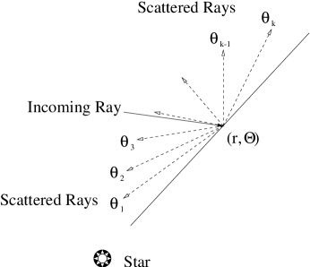
Figure 2: [Left] The scattering angle, $\omega$, is defined by the acute angle between the directions of incident and scattering. [Right] In the anisotropic scattering mode, the incoming angle-integrated intensity available at a given grid is redistributed into each of the $\theta$ directions according to the weights computed by the scattering phase function.

Appendix C Shell Properties

In 2-Dust, the normalized density profile of the shell, $\rho(r,\Theta)$, may be defined by users as a Fortran function. Then, the density at the inner radius along the equator, $\rho_{\rm min}$, must be determined from the given optical depth at the given frequency through

$$\tau_{\nu}=k_{\nu}\rho_{\rm min}\int_{r_{\rm min}}^{r_{\rm max}}\rho\left(r,\frac{\pi}{2}\right)dr.$$ (C1)

In the above case where there is only one type of dust species, the cross section is in units of cm² and the density is in units of cm^-3. However, the dust shell may have a number of distinct dust layers to account for, for example, a shell with distinct composition layers (e.g., reflecting a possible surface composition change of the central star) and a shell having layers with different size distributions (e.g., reflecting some dynamical effects such as grain-grain collisions).

When multiple composition layers are present, there would be a difference in physical characteristics of the shell depending on whether the mass density (g cm^-3) or number density (cm^-3) of the dust grains is assumed to be continuous. For example, the mass density continuity is needed to create a single-composition shell having multiple layers of distinct dust size distributions (i.e., the number density is expected to be discontinuous at the size distribution boundary). It is reasonable to assume that dust grains aggregate and/or fragment, for some physical reason, into grains of different sizes while keeping the overall mass density unchanged. On the other hand, the number density continuity is a necessary assumption if one sets up a dust shell with multiple composition layers following the heterogeneous nucleation theory. Dust grains are thought to form only when there are nucleation sites, i.e., the existing grains on which a mantle of differing composition can form. If this is the case, the number density remains to be continuous at the composition boundaries (i.e., the mass density is expected to be discontinuous).

With multiple composition layers, equation (C1) reads

$$\tau_{\nu}=\rho_{\rm min}\sum_{m=1}^{n}\int_{r_{m-1}}^{r_{m}}k_{\nu}^{(m)}\rho\left(r,\frac{\pi}{2}\right)dr,$$ (C2)

where $r_{m}$ and $k_{\nu}^{(m)}$ are respectively the outer boundary and the total extinction cross section for the $m$ th composition layer and $n$ is the total number of layers. Depending on the physical considerations specific to the problem to be solved, $\rho_{\rm min}$ can be either the mass or number density. This distinction, of course, would affect the physical meaning of the cross sections.

Once $\rho_{\rm min}$ is determined, the total dust mass of the shell can be calculated by integrating over the entire shell. Then, the rate of dust mass loss can be determined by dividing the total dust mass in the shell by the age of the shell estimated from the wind crossing time in the shell.

References

- Bohren & Huffman (1983) Bohren, C. F. & Huffman, D. R. 1983, Absorption and Scattering of Light by Small Particles (New York: John Wiley & Sons)
- Collison & Fix (1991) Collison, A. & Fix, J. 1991, ApJ, 368, 545
- Cornette & Shanks (1992) Cornette, W. M., & Shanks, J. G. 1992, Appl. Opt., 31, 3152
- Dayal et al. (1998) Dayal, A., Hoffmann, W. F., Bieging, J. H., Hora, J. L., Deutsch, L. K., & Fazio, G. G. 1998, ApJ, 492, 603
- Dorschner et al. (1995) Dorschner, J., Begemann, B., Henning, T., Jäger, C., & Mutschke, H. 1995, A&A, 300, 503
- Dullemond & Turolla (2000) Dullemond, C. P., & Turolla, R. 2000, A&A, 360, 1187
- Efstathiou & Rowan-Robinson (1990) Efstathiou, A. & Rowan-Robinson, M. 1990, MNRAS, 245, 275
- Ivezić, Nenkova, & Elitzur (1999) Ivezić, Ž., Nenkova, M., & Elitzur, M. 1999, User Manual for DUSTY, University of Kentucky Internal Report
- Jäger et al. (1994) Jäger, C., Mutschke, H., Begemann, B., Dorschner, J., & Henning, Th. 1994, A&A, 292, 641
- Jäger, Mutschke, & Henning (1998) Jäger, C., Mutschke, H., & Henning, Th. 1998, A&A, 332, 291
- Jura (1994) Jura, M. 1994, ApJ, 434, 713
- Jura, Chen, & Werner (2000) Jura, M., Chen, C., & Werner, M. W. 2000, ApJ, 544, L141
- Kemper et al. (2002) Kemper, F., Jäger, C., Waters, L. B. F. M., Henning, Th., Molster, F. J., Barlow, M. J., Lim, T., & de Koter, A. 2002, Nature, 415, 295
- Kim, Martin, & Hendry (1994) Kim, S.-H., Martin, P. G., & Hendry, P. D. 1994, ApJ, 422, 164
- Kunasz & Auer (1988) Kunasz, P. B., & Auer, L. H. 1988, J. Quant. Spec. Radiat. Transf., 39, 67
- Lefèvre, Daniel, & Bergeat (1983) Lefèvre, J., Daniel, J.-Y., & Bergeat, J. 1983, A&A, 121, 51
- Lopez, Mékarnia, & Lefèvre (1995) Lopez, B., Mékarnia, D., & Lefèvre, J. 1995, A&A, 296, 752
- Mathis, Rumpl, & Nordsieck (1977) Mathis, J. S., Rumpl, W., & Nordsieck, K. H. 1977, ApJ, 217, 425
- Meixner et al. (1999) Meixner, M., Ueta, T., Dayal, A., Hora, J. L., Fazio, G., Hrivnak, B. J., Skinner, C. J., Hoffmann, W. F., & Deutsch, L. K. 1999, ApJS, 122, 221.
- Meixner et al. (2002) Meixner, M., Ueta, Bobrowsky, M., & Speck, A. K. 2002, ApJ, 571, 936
- Men’shchikov & Henning (1997) Men’shchikov, A. B., & Henning, Th. 1997, 318, 879
- Molster et al. (2002) Molster, F. J., Waters, L. B. F. M., Tielens, A. G. G. M., & Barlow, M. J. 2002, A&A, 382, 184
- Sedlmayr (1994) Sedlmayr, E. 1994, in Molecules in the Stellar Environment, ed. U. G. Jørgensen (Berlin: Springer-Verlag), 163
- Siebenmorgen, Krügel, & Mathis (1992) Siebenmorgen, R., Kr[̈u]gel, E., & Mathis, J. S. 1992, A&A, 266, 501
- Skinner et al. (1994) Skinner, C. J., Meixner, M., Hawkins, G. W., Keto, E., Jernigan, J. G., & Arens, J. F. 1994, ApJ, 423, 135
- Skinner et al. (1997) Skinner, C. J., Meixner, M., Barlow, M. J., Collison, A. J., Justtanont, K., Blanco, P., Piña, R., Ball, J. R., Keto, E., Arens, J. F., & Jernigan, J. G. 1997, A&A, 328, 290
- Smith et al. (2002) Smith, N., Gehrz, R. D., Hinz, P. M., Hoffmann, W. F., Mamajek, E. E., Meyer, M. R., Hora, J. L. 2002, ApJ, 567, 77L
- Spagna, Leung, & Egan (1991) Spagna, G. F. Jr., Leung, C. M., & Egan, M. P. 1991, ApJ, 379, 232
- Speck (1998) Speck, A. K. 1998, PhD. Thesis, University College London
- Ueta, Meixner, & Bobrowsky (2000) Ueta, T., Meixner, M., & Bobrowsky, M. 2000, ApJ, 528, 861
- Ueta et al. (2001a) Ueta, T., Meixner, M., Dayal, A., Deutsch, L.K., Fazio, G.G., Hora J.L., & Hoffmann, W.F. 2001a, ApJ, 548, 1020
- Ueta et al. (2001b) Ueta, T., Meixner, M., Hinz, P.M., Hoffmann, W.F., Brandner, W., Dayal, A., Deutsch, L.K., Fazio, G.G., & Hora, J.L. 2001b, ApJ, 557, 831
- van de Hulst (1957) van de Hulst, H. C. 1957, Light Scattering by Small Particles (New York: John Wiley & Sons)
- Waters et a. (1996) Waters et al. 1996, A&A, 315, L361
- Weinberger et al. (2002) Weinberger, A. J., Becklin, E. E., Schneider, G., Chiang, E. I., Lowrance, P. J., Silverstone, M., Zuckerman, B., Hines, D. C., & Smith, B. A. 2002, ApJ, 566, 409