Structure and mass distribution of spiral galaxies at intermediate redshifts

Using the HST archive WFPC2 observations and rotation curves measured by Vogt et al. (vogt1 (1996)), we constructed self-consistent light and mass distribution models for three disk galaxies at redshifts $z=0.15,0.90$ and $0.99$. The models consist of three components: the bulge, the disk and the dark matter. Spatial density distribution parameters for the components were calculated. After applying k-corrections, mass-to-light ratios for galactic disks within the maximum disk assumption are $M/L_{B}=$ 4.4, 1.2 and 1.2, respectively. Corresponding central densities of dark matter halos within a truncated isothermal model are 0.0092, 0.028 and 0.015 in units $\rm M_{\sun}/pc^{3}$. The light distribution of the galaxies in outer parts is steeper than a simple exponential disk.

1 Introduction

The study of dark matter halo properties and central densities allows to constrain possible galaxy formation models and large scale stucture formation scenarios (Primack primack (2002); Khairul Alam et al. khai (2002)). It is interesting to analyse the corresponding data at different redshifts. For this kind of analysis it is needed to know both the distribution of visible and dark matter. Unfortunately, the structure and mass distribution of stellar populations, and therefore, the discrimination between visible and dark matter in very distant galaxies is still largely unknown.

General morphological evolution of galaxies at intermediate and high redshifts has been studied, for example by Smail et al. (smai (1997)), Andreon et al. (andr (1997)), Lubin et al. (lubi (1998)), Fabricant et al. (fabr (2000)), van den Bergh et al. (berg (2000)), van Dokkum et al. (2001a ), La Barbera et al. (barb (2002)), Im et al. (im (2002)). Several statistical correlations and color gradients in clusters at redshifts $z=0.3-1$ have been studied by Stanford et al. (stan (1998)), Ziegler et al. (zieg1 (1999)), van Dokkum et al. (dokk2 (2000)), Saglia et al. (sagl (2000)), Tamura & Ohta (ta:oh (2000)). More sophisticated correlation parameters for elliptical galaxies, the Fundamental Plane parameters involving dynamical information, have been determined by Kelson et al. (kels1 (1997)), van Dokkum et al. (dokk1 (1998), 2001b ), Kelson et al. (kels2 (2000)), Treu et al. (treu (2001)).

These studies indicate that most of the stellar content of early-type galaxies has formed at redshifts $z>2-3$, and has passed normal chemical evolution and there is no significant age difference between field and cluster galaxies. Within the standard $\Lambda$CDM model, field ellipticals must be younger than cluster ellipticals. On the other hand, the fraction of early-type galaxies in clusters is smaller and the fraction of E+A (post-starburst) galaxies is higher at intermediate redshifts, indicating some morphological transformations from $z\sim 1$ to the present time. Theoretical models indicate that truncation of star formation rate can successfully explain this kind of morphological changes (van Dokkum & Franx, do:fr2 (2001); Bicker et al. bick (2002)).

Less is known about the structure of spiral galaxies at intermediate redshifts. For analysing the emission line profiles of disk galaxies, it is needed to distinguish the rotation and dispersion components. Spectrograph slit width is usually only slightly smaller than galactic dimensions which makes derived rotation curves uncertain and often only maximum values of rotation velocities can be estimated.

By now the maximum values of rotation velocities have been measured for distant galaxies up to redshift $z=1.34$ (Colless et al. coll (1994); Forbes et al. forb (1996); Rix et al. rix (1997); Simard & Pritchet si:pr (1998), Schade et al. scha (1999); Mallen-Ornelas et al. mall (1999); Briggs et al. brig (2001); van Dokkum & Stanford do:st (2001)). When plotted to the Tully-Fisher diagram, these measurements allow to compare the measured galaxies with the local ones. Rotation curves of very distant galaxies have been measured only by Vogt et al. (vogt1 (1996), vogt2 (1997)), Ziegler et al. (zieg2 (2002)) and Steidel et al. (stei (2002)). These data allow more detailed modeling of the structure of corresponding galaxies, especially if the curve extends beyond the solid-body rotation part.

To construct a self-consistent photometrical and dynamical model of a galaxy, both surface photometry and rotation curve data are needed. In the case of galaxies at intermediate redshifts the typical scale is $5-10$ kpc per arcsec and in order to determine the parameters of galactic components, it is recommendable to use also high-resolution HST photometry in addition to other photometrical data.

For our modeling, the galaxies had to match the following criteria. Their velocity profiles had to be undisturbed, symmetric with respect to the galactic centre and with sufficient extent. Galaxies seen almost face-on were not suitable due to uncertainties of the inclination angle of the galactic plane. We also could not use galaxies being seen edge-on, because for these galaxies the surface brightness distribution is largely influenced by galactic absorption. For detailed modeling, we selected three galaxies with rotation curves measured by Vogt et al. (vogt1 (1996)): 074-2237, 064-4412, 094-2210. For deriving the surface brightness distribution of these galaxies, we used images from the HST archive. General properties of these galaxies are given in Table 1. In the present work we take $H_{0}=65$ km/s/Mpc and $q_{0}=0.5.$

Table 1: General galactic parameters.

Namea	RA	DEC	Hubble	$z^{a}$	Scale	Inclin.a	$M_{B}^{b}$
	(2000)	(2000)	type		(kpc/”)	(deg)
074-2237	$\rm 14^{h}17^{m}45.4^{s}$	$\rm 52^{o}27^{\prime}59.9^{\prime\prime}$	Sc	0.154	2.76	80	$-20.0$
064-4412	$\rm 14^{h}17^{m}53.4^{s}$	$\rm 52^{o}29^{\prime}41.1^{\prime\prime}$	Sc	0.988	6.71	68	$-20.6$
094-2210	$\rm 14^{h}17^{m}31.3^{s}$	$\rm 52^{o}26^{\prime}08.8^{\prime\prime}$	Sbc	0.900	6.65	60	$-21.5$

• Galactic names and redshifts are from Vogt et al. (vogt1 (1996)), inclinations are from Simard et al. (sima (2002))
  

• Absolute B-magnitudes in galactic rest-frame are from our models (Sect. 4)
  

2 Photometrical structure

The images of all three galaxies were retrieved from the archive of the Hubble Space Telescope (WFPC2, observational programs 5090 and 5109, filters F814W and F606W). For processing we used pipeline-reduced on-the-flight calibrated images. 12 exposures in both colors were available for the galaxy 074-2237 and 4 exposures for the other two. Details about image processing and derivation of surface brihtness profiles are described in Tamm & Tenjes (ta:te (2001)). Here we summarize only basic steps, bringing out especially these aspects which differ from the previous processing. Processing was done with IRAF/STSDAS packages.

In order to elliminate cosmic rays, exposures were combined using the STSDAS task combine (option crrej). Before estimating the background, combined images were filtered to smooth down noises (task adaptive). We found no evidence of galaxy distortion caused by adaptive filtering. As the investigated galaxies were rather small in CCD frames, it was sufficient to subtract in all cases a constant background value from the images. Background values were determined by interpolating the values of the surrounding regions of the galaxies. This stage differs from the one we have used earlier. New on-the-flight calibration of the HST archive data has improved the quality of the original images, especially in the case of the galaxy 064-4412. The background levels were (in WFPC2 intensity counts) 11.7 (I)and 19.8 (V) for the galaxy 074-2262; 6.40 (I) and 7.25 (V) for the galaxy 064-4412; 6.25 (I) and 7.25 (V) for the galaxy 094-2210. Images of the three galaxies after background subtraction are given in Fig. 1.

Figure 1: Images of the galaxies (from left to right) 074-2237, 064-4412, and 094-2210 in F814W color after background subtraction.

The resulting images were deconvolved using the Lucy-Richardson algorithm for modeling PSF with the help of TinyTim 6.0. V-band images of 064-4412 and 094-2210 were not deconvolved, because due to a low signal-to-noise ratio deconvolution process gave unrealistic results. In order to calculate isophotes, task ellipse was used. The fitting process was carried out several times for each of the galaxies in order to estimate and reduce uncertainties. The scatter of the dots in Fig. 2 illustrates uncertainties of isophote fitting.

Figure 2: Surface brightness distribution of the galaxies (from left to right) 074-2237, 064-4412, and 094-2210 in I and V colors. Both original and deconvolved profiles are given.

Before final calibration, we estimated the corrections of the luminosity flux for the geometric distortion and the charge transfer efficiency effect of the WFPC2 (Holtzman et al. 1995a ). We added 2% to the signal to compensate for the geometric distortion of 064-4412 and 094-2210 and 1.5% in the case of 074-2237. To transfer the luminosity counts into standard Johnson magnitudes, the calibration described by Holtzman et al. (1995b ) (H95) was used. For the filter F814W, we used the flight photometric system Eq. (8) and the coefficients from Table 7 in H95:

$$I=-2.5\leavevmode\nobreak\ \log\leavevmode\nobreak\ (DN/t)-0.062(V-I)+0.025(V-I)^{2}+$$

$$20.839+2.5\log(GR)+0.1+0.05.$$

For F606W filter, we used the synthetic calibration Eq. (9) and coefficients from Table 10 in H95:

$$V=-2.5\leavevmode\nobreak\ \log\leavevmode\nobreak\ (DN/t)+0.254(V-I)+0.012(V-I)^{2}+$$

$$22.093+2.5\log(GR)+0.1+0.05.$$

Here GR is gain ratio as defined in H95, the term 0.1 corrects the formula for infinite aperture and 0.05 is the correction due to long exposures. $V-I$ was calculated iteratively. Luminosity flux was corrected for the cosmological distortion by a factor $(1+z)^{4}.$

Luminosities have been corrected for absorption in our Galaxy according to Schlegel et al. (schl (1998)).

We estimated the k-correction in two ways. First, the observed colors were transformed to such standard colors for which the k-correction would be minimal. For this we used the method described in van Dokkum & Franx (do:fr1 (1996)) and Kelson et al. (kels2 (2000)). At redshift $z=0.15$ a suitable transformation would be from V to B and for redshifts 0.9 and 0.99 from I to B. For all three galaxies we used synthetic spectra of a Sbc–Scd galaxy derived by Coleman et al. (cole (1980)). Zero points relating AB magnitudes and Johnson magnitudes were taken from Frei & Gunn (fr:gu (1994)). Second, the k-corrections were estimated by using the chemical evolution models by Schulz et al. (schu (2002)). Again, at $z=0.15$ V color was transformed to B color, assuming the rest-frame $\rm(B-V)=0.63$, at redshifts 0.90 and 0.99 I color was transformed to B color, assuming the rest-frame $\rm(B-I)=1.76$. For the nearest galaxy, we took solar metallicity, for the two others $Z=0.008$. The results obtained by two methods nearly coincide in the case of the nearest galaxy, for more distant galaxies the agreement is within $\pm 0.15^{\rm m}$. Averaging the results of the two methods yields the following relations:

$$\begin{array}[]{ll}B(z=0.15)&=V+0.32,\\ B(z=0.90)&=I+0.90,\\ B(z=0.99)&=I+1.02.\\ \end{array}$$

Here $V$, $I$ and $(V-I)$ are observed Johnson magnitudes and $B$ is the Johnson magnitude in galactic rest-frame. The final galactic surface brightness profiles are presented in Fig. 3 by open circles. Error bars characterize uncertainties of both background determination and isophote construction.

Figure 3: Surface brightness distribution of the galaxies 074-2237, 064-4412, and 094-2210 (from left to right) in rest-frame B color (open circles). Solid line – surface brightness distribution of the best fit model, dashed lines – surface brightness distribution of model components.

3 Galactic models

Although several stellar populations can be discriminated in spiral galaxies, in the case of modeling very distant galaxies it is reasonable to limit the main stellar components to two – the bulge and the disk. Parameters of any other stellar component (central nucleus, metal poor halo, thick disk) could not be determined at present from available photometric observations. To construct a dynamical model, a dark matter component – the dark halo must be added to visible components. Of course, the photometrical and dynamical models must be mutually consistent.

When handling only surface photometry data, it is convenient to describe the galactic structure with the help of some simple parametric formulae for the surface density. Most common formulae are the de Vaucouleurs formula, the exponential law or the more general Sérsic formula. Most flexible is the Sérsic formula with an additional parameter, allowing to control the steepness of the surface density decrease (Sérsic sersic (1968)). Density distribution parameters must be determined e.g. by the least squares method. Using also kinematic data and constructing a dynamical model consistent with the photometry, the same density distribution law must be used for rotation curve modeling (and for velocity dispersion curve, if possible). In the case of the Sérsic formula, it can be done for spherical systems with an integer Sérsic index $m$ (Mazure & Capelato ma:ca (2002)). For a noninteger index and ellipsoidal surface density distribution a consistent solution for rotation curve calculations is not known.

In the present paper, the density distribution parameters are determined by the least squares method and they can have any value. Thus, it is not reasonable to use the Sérsic law for surface density distribution. It is more physical to start from the spatial density law. An analytical expression for spatial densities, reproducing well the Sérsic formula, was derived by Trujillo et al. (truj2 (2002)). Although this formula is useful, we decided to use for the bulge and for the disk an analyticaly simpler form (1), allowing to use more easily least-square fitting simultaneously for light distribution and rotation curve.

In our model the visible part of a galaxy is given as a superposition of the bulge and the disk. The spatial density distribution of every visible component (the bulge and the disk) is approximated by an inhomogeneous ellipsoid of rotational symmetry with constant axial ratio $q$ and the density distribution law (Einasto einasto (1969))

$$\rho(a)=\rho(0)\exp[-(a/(ka_{0}))^{1/N}],$$ (1)

where $\rho(0)=hM/(4\pi qa_{0}^{3})$ is the central density, $M$ is the component mass. Next, $a=\sqrt{R^{2}+z^{2}/q^{2}}$, where $R$ and $z$ are two cylindrical coordinates. $a_{0}$ is the harmonic mean radius

$$a_{0}^{-1}=\int_{0}^{\infty}a^{-1}dM,$$ (2)

where $dM=4\pi qa^{2}\rho(a)da$ is the mass of the ellipsoidal shell of thickness $da$. Coefficients $h$ and $k$ are normalizing parameters, depending on $N$, which allows to vary the density behavior with $a$. The harmonic mean radius characterizes rather well the real extent of a component, independently of the parameter $N$. The definition of normalizing parameters $h$ and $k$ and their calculation is described in Tenjes et al. (tenj1 (1994)), Appendix B. Eq. 1 allows sufficiently precise numerical integration and has a minimum number of free parameters.

The dark matter (DM) distribution is represented by a spherical isothermal law

$$\rho(a)=\cases{\rho(0)([1+({a\over a_{c}})^{2}]^{-1}-[1+({a^{0}\over a_{c}})^{2}]^{-1})&$a\leq a^{0}$\cr 0&$a>a^{0}$.\cr}$$ (3)

Here $a^{0}$ is the outer cutoff radius of the isothermal sphere.

The density distributions for the bulge and the disk were projected along the line of sight, divided by their mass-to-luminosity ratios $f$ and their sum gives us the surface brightness distribution of the model

$$L(A)=2\sum_{i=1}^{2}{q_{i}\over Q_{i}f_{i}}\int_{A}^{\infty}{\rho_{i}(a)a\leavevmode\nobreak\ da\over(a^{2}-A^{2})^{1/2}},$$ (4)

where $A$ is the major semiaxis of the equidensity ellipse of the projected light distribution, $Q_{i}$ are their apparent axial ratios $Q^{2}=\cos^{2}\gamma+q^{2}\sin^{2}\gamma$. The angle between the plane of a galaxy and the plane of the sky is denoted by $\gamma$. Summation index $i$ designates two visible components, the bulge and the disk.

The masses of the components we determined from the rotation law

$$v_{i}^{2}(R)=4\pi q_{i}G\int_{0}^{R}{\rho_{i}(a)a^{2}da\over(R^{2}-e_{i}^{2}a^{2})^{1/2}},$$ (5)

$$V^{2}(R)=\sum_{i=1}^{3}v_{i}^{2}(R),$$ (6)

where $G$ is the gravitational constant, $e=\sqrt{1-q^{2}}$ is eccentricity, and $R$ is the distance in the equatorial plane of the galaxy. Summation is over all three components now.

Model parameters $a_{0}$, $q$, $L_{B}$, $M$ and $N$ for the bulge and the disk were determined by a subsequent least-squares approximation process. As the first step, we made a crude estimation of the population parameters. The purpose of this step is only to avoid obviously unphysical parameters – relations (4) and (5) are nonlinear and fitting the model to the observations is not a straightforward procedure. Next a mathematically correct solution for each galaxy was found. Details of the least squares approximation and the general modeling procedure were described by Einasto & Haud (ei:ha (1989)), Tenjes et al. (tenj1 (1994), tenj2 (1998)).

The rotation curves of the galaxies 074-2237, 064-4412, 094-2210 have a rather small extent (see Figs. 4–6). We do not have any additional information about the dynamics of these galaxies at large galactocentric radii. For this reason, the outer cutoff radius of the DM component remains undetermined at present. We fixed $a^{0}=5a_{0}$ on the basis of the structure of nearby galaxies. This value influences the rotation curve behavior only in extreme outer regions of galaxies and does not influence our results. Then we assumed by analogy with nearby galaxies that the rotation curve of these galaxies remains flat at least up to 30 kpc (Sofue & Rubin so:ru (2001)).

As we have no information about velocity dispersions in the central regions of our galaxies we can calculate only the circular velocities (Eqs. 5–6). If the value of velocity dispersions is comparable to the value of rotational velocity at a particular distance, the latter does not correspond to the value of circular velocity. The difference is known in galactic dynamics as the asymmetric drift. Typical emission-line dispersions in galaxies at intermediate redshifts are 30–100 km/s (Koo et al. koo (1997); Guzman et al. guzm (1997); Im et al. im1 (2001)). Thus, within central $0.5\arcsec-0.7\arcsec$ model velocities must be higher than the observed rotational velocities.

4 Results and discussion

Calculated from our photometry, the total apparent Johnson V luminosity of the galaxy 074-2237 is $V=19.28\pm 0.05$, which coincides well with the $\rm V_{\rm 606}$ luminosity estimates by Vogt et al. (vogt1 (1996)) 18.70 and Simard et al. (sima (2002)) 18.78. The mean apparent color index is $\rm(V-I)=1.5\pm 0.2$. The difference between the Johnson V and $\rm V_{606}$ is $0.49^{m}$, if $\rm(V-I)=$1.5.

The calculated total apparent Johnson I luminosity of the galaxy 064-4412 is $I=22.43$, which also coincides well with the $I_{\rm 814}$ luminosity estimates by Vogt et al. (vogt1 (1996)) 22.38 and by Simard et al. (sima (2002)) 22.33. The mean apparent color index is $\rm(V-I)=2.2$. The difference between the Johnson I and $\rm I_{814}$ is $0.12^{m}$ if $\rm(V-I)=$2.3.

The total apparent Johnson I luminosity of the galaxy 094-2210 from our photometry is $I=21.47$. The $I_{\rm 814}$ luminosity estimate by Vogt et al. (vogt1 (1996)) is 21.41 and by Simard et al. (sima (2002)) it is 21.21. The mean apparent color index is $\rm(V-I)=2.4$.

Table 2: Galactic model parameters.

Name	$q$	$a_{0}$	$M$	$M/L_{B}$	$N$	$h$	$k$	$L_{B}$	$M^{a}$
		(kpc)	$\mathrm{1}0^{10}M_{\sun}$				$\mathrm{1}0^{10}L_{\sun}$	$\mathrm{1}0^{10}M_{\sun}$
074-2237
bulge	0.7	1.1	(0.2)	2.2	0.75	2.459	0.7822	0.092	(0.05)
disk	0.1	7.1	6.4	4.4	0.50	1.571	1.128	1.46	6.5
dark matter		60.	(170.)			14.82	0.1511		(170.)
064-4412
bulge	0.7	1.5	(0.3)	0.78	0.51	1.592	1.117	0.38	(0.05)
disk	0.1	7.3	2.7	1.17	0.43	1.397	1.229	2.30	3.0
dark matter		40.	(150.)			14.82	0.1511		(150.)
094-2210
bulge	0.7	1.7	(2.1)	1.9	0.67	2.115	0.8801	1.08	(0.7)
disk	0.1	9.3	6.4	1.19	0.25	1.080	1.445	5.38	8.0
dark matter		60.	(250.)			14.82	0.1511		(250.)

• Mass distribution model with low bulge masses (upper panels in Figs 4–6).
  

The final two-component models fit the photometric B-profiles with a mean relative error of 0.2–0.5 per cent. For the fitting of the rotation curves, we constructed two models for each galaxy. One kinematical model corresponds to the mathematically best fit at all distances, even in the central regions. However, due to the arguments given in the last paragraph of the previous section, this model is unphysical, because it underestimates the bulge mass. Therefore, a second model was constructed with the bulge mass fixed at higher values. At present we have no independent basis to estimate the bulge mass. We hope that two different models allow the reader to understand how the bulge mass variation influences the overall behaviour of rotation curves in all three concrete cases. Real bulge masses and thus also mass-to-light ratios may be higher than the values resulting from Table 2. To derive real bulge mass-to-light ratios, additional observations (central stellar velocity dispersions) are needed.

The parameters of the final models (the axis ratio $q$, the harmonic mean radius $a_{0}$, the total mass of the population $M$, the structural parameter $N$, the dimensionless normalizing constants $h$ and $k$, B-luminosities and corresponding mass-to-light ratios) are given in Table 2. Bulge and DM masses are given in parentheses to indicate that on the basis of present observational data it is not possible to determine these values uniquely. The last column in Table 2 gives the masses for low bulge mass models. The final models are denoted by thick solid lines in Figs. 3–6. Models of individual visible components are represented by dashed lines, the model of the dark matter component by a thin solid line. In Table 3, calculated from the models, integrated parameters are given: apparent I-band magnitude, total mass of the visible matter, total intrinsic luminosity and mass-to-light ratio of the visible matter.

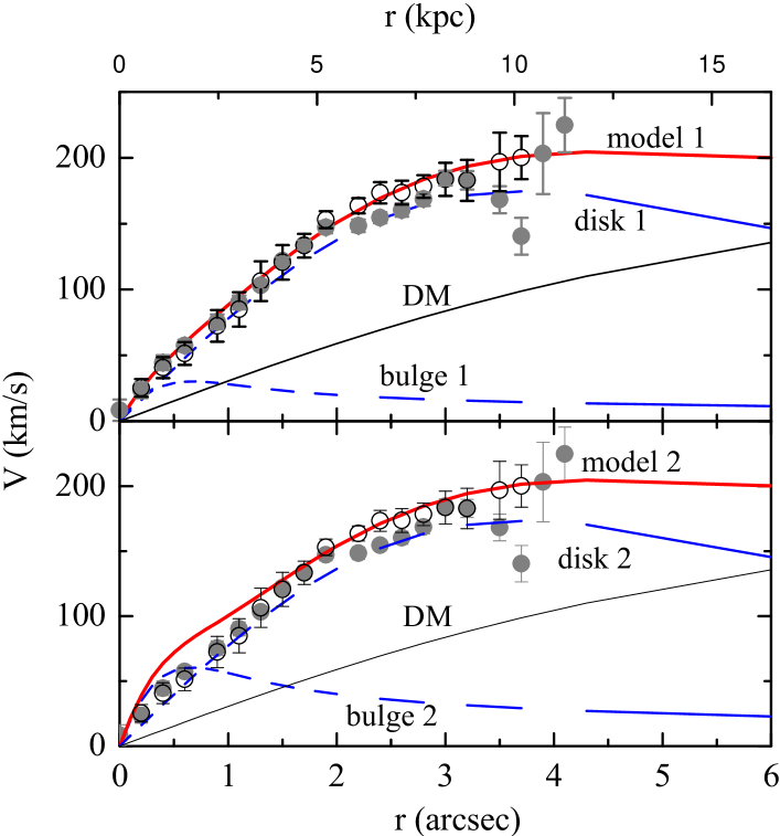
Figure 4: Rotation curve of the galaxy 074-2237. Open and grey circles – observations by Vogt et al. (1996) at the opposite sides of the galaxy, thick solid line – rotation curve from the mass model, dashed lines – rotation velocities due to visible components, thin solid line – rotation velocities due to the dark matter component. Upper panel (model 1) corresponds to low bulge mass, lower panel (model 2) corresponds to higher bulge mass.

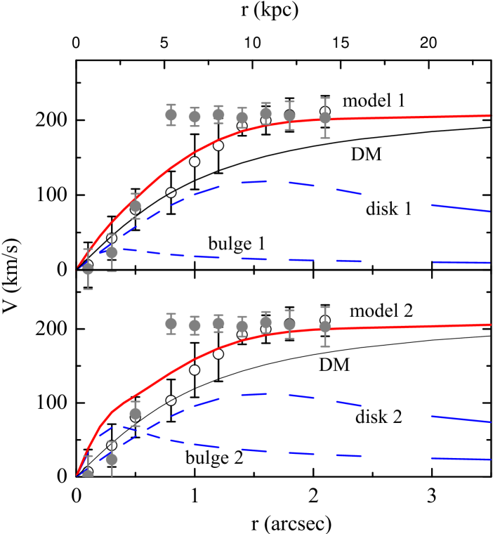
Figure 5: Rotation curve of the galaxy 064-4412. Designations are the same as in Fig. 4.

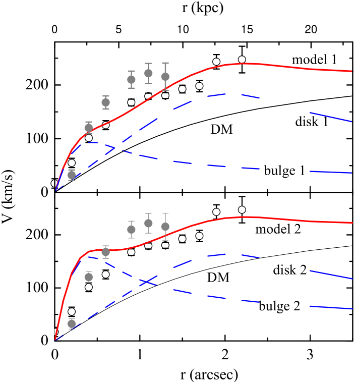
Figure 6: Rotation curve of the galaxy 094-2210. Designations are the same as in Fig. 4.

Table 3: Derived integrated parameters from models.

Namea	$m_{I}$	$M_{\rm vis}$	$L_{B}$	$(M/L)_{\rm vis}$
	(mag)	$\rm 10^{10}M_{\sun}$	$\rm 10^{10}L_{\sun}$
074-2237	17.78	6.6	1.55	4.3
064-4412	22.43	3.0	2.68	1.1
094-2210	21.47	8.4	6.46	1.3

It is interesting to compare the central surface brightnesses of galactic disks with the results obtained for local galaxies. For the galaxies modeled here, the central brightnesses of disks are $\mu_{B}(0)=$ 21.4, 21.3, 21.1. The mean value for two galaxies at redshifts $z=0.9-1$ is $\mu_{B}(0)=21.2$. For local galaxies the original value by Freeman (freeman (1970)) was 21.65. However, this value probably depends on the galactic morphological type and luminosity, and thus has considerable scatter (Graham & de Blok gr:bl (2001)). For galaxies at redshifts $z=0.5-1$ Schade et al. (scha2 (1996)) derived $\mu_{B}(0)=20.0$, when transformed to conventional broadband magnitudes, but also with a rather significant scatter. Our values are clearly higher. However, it must be taken into account that central brightnesses of disks have been determined by Schade et al. (scha2 (1996)) within the assumption of exponential disks and $r^{1/4}$ bulge. When fitting the disks of our two higher redshift galaxies with parameters $N=1$, the resulting disk central brightnesses are brighter by 0.6 mag, i.e. the mean value is $\mu_{B}(0)=20.6$. Disk central brightness is sensitive also to bulge parameters. Our bulge profile is quite different from the $r^{1/4}$ law. And finally, when taking into account also the uncertainties in k-correction, our values for the disk central brightnesses are not peculiar.

Figure 3 shows that the light distribution in outer parts of the galaxies studied in the present paper is rather steep (the parameter $N$ is small). In all cases, the disk density distribution in outer parts is steeper than for a simple exponential disk. Central concentration parameters (Trujillo et al. truj1 (2001)) for these galaxies are rather small, about 0.15. Steep decrease of the surface brightness in outer parts of galaxies may be the result of the outer truncation of the disk. According to Pohlen et al. (pohl (2000)), the truncation occurs at distances of about 3 disk scale lengths. In the case of galaxies studied here, the surface photometry does not extend to so large distances.

The central density of the dark matter $\rho(0)=hM/(4\pi a_{0}^{3}),$ characterizing the rotation velocity gradient at the center caused by the dark halo, is rather well determined from observations and nearly independent of the choice of the dark halo outer cutoff radius. Calculated from our models, the central densities of DM components are $\rho(0)=$ 0.0092, 0.028, and 0.015 in units $\rm M_{\sun}/pc^{3}$. It is important to stress that these values are calculated for maximum disk models and are thus the lower limits. This must be taken into account especially in the case of the first value (the galaxy 074-2237) where models with lower disk mass and higher DM density give equally good fit for the rotation curve. The visible and DM masses become equal for this galaxy at $R=17$ kpc in our maximum disk model. A mass distribution model of the galaxy 074-2237 was conctructed also by Fuchs et al. (fuch (1996)) who used for mass determination a model of spiral arm formation via swing-amplification. They concluded that in order to create a two-armed spiral structure, higher DM densities are needed when compared with the maximum disk models. According to their model, the central DM density of 074-2237 is 0.025.

It is possible to construct mass distribution models for galaxies without assuming the existence of a DM component. Corresponding models are given in Figs 7–9. It is seen that the calculated rotation curves start to decrease after the last observed point of the rotation curves. Thus, within the available at present observations, the models without any dark halo fit well with observations.

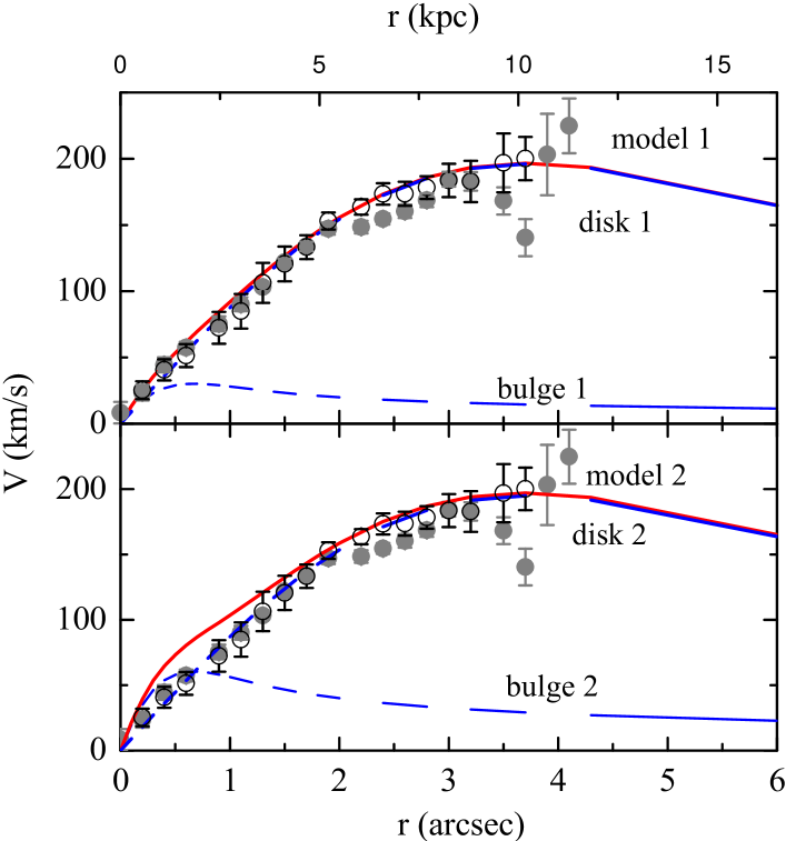
Figure 7: Rotation curve model of the galaxy 074-2237 without the dark matter component. Disk masses are 8.2 (disk 1) and 8.1 (disk 2) in units of $\rm 10^{10}M_{\sun}$. Designations are the same as in Fig. 4.

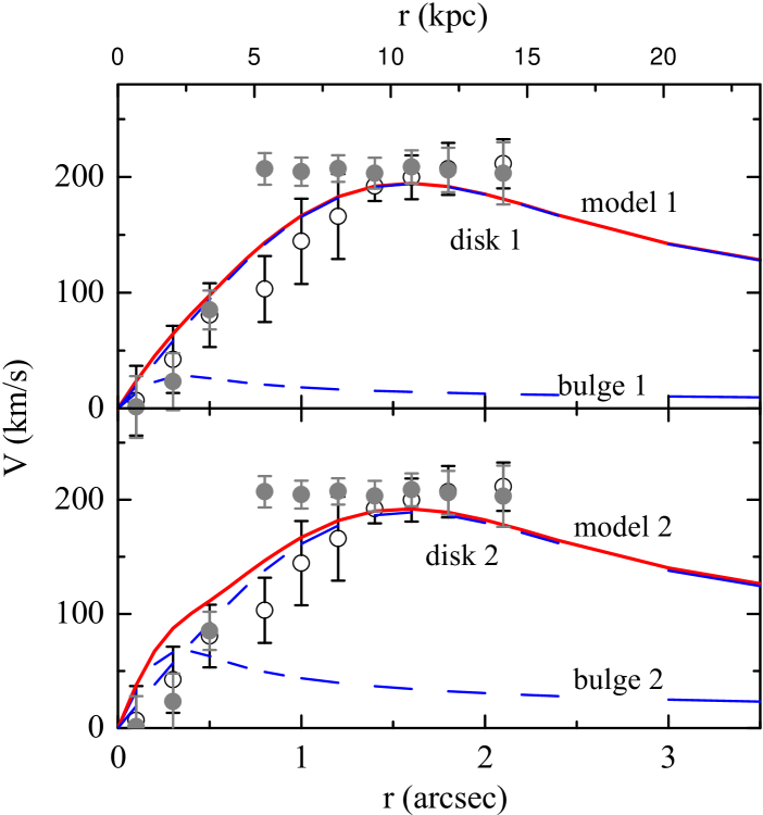
Figure 8: Rotation curve model of the galaxy 064-4412 without the dark matter component. Disk masses are 8.1 (disk 1) and 7.7 (disk 2) in units of $\rm 10^{10}M_{\sun}$. Designations are the same as in Fig. 4.

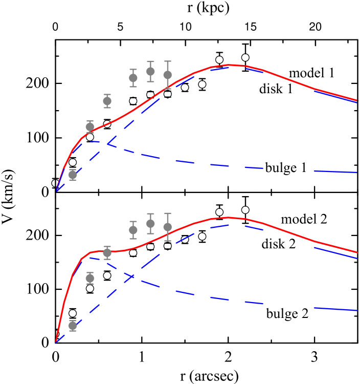
Figure 9: Rotation curve model of the galaxy 094-2210 without the dark matter component. Disk masses are 12.5 (disk 1) and 11.4 (disk 2) in units of $\rm 10^{10}M_{\sun}$. Designations are the same as in Fig. 4.

As mentioned earlier, due to the limitied extent of rotational curves it is not possible to determine any parameters of the DM distribution. Figures 7–9 show that rotation curves can be well fitted without DM. However, we think that there are enough independent arguments in support of the existence of DM and thus, realistic models must include a DM component. For this reason, on the basis of nearby galaxies weumed that rotation curves remain flat up to the distances of about 30 kpc (see Sofue & Rubin so:ru (2001)). This assumption still does not enable to determine the total DM mass and its characteristic radius. Only the central density of the DM component can be found. Therefore, the mass and the radius of the DM component given in Table 2 are simply fixed. It is possible to fix, e. g. the DM mass two times smaller, decreasing correspondingly the DM radius in a way that the central density remain unchanged. The central density of DM can be dermined from models within the assumption of the flatness of rotation curves. The central density of DM is not sensitive to the uncertainties of bulge mass.

The central density of the dark matter distribution is a parameter allowing to constrain possible cosmological models and corresponding parameters at early periods of structure formation (see eg. Navarro & Steinmetz na:st (2000), Shapiro & Iliev sh:il (2002), Khairul Alam et al. khai (2002), Zentner & Bullock ze:bu (2002)). We think it is reasonable to derive also the central DM densities at different redshifts. In the present paper we have used only one density distribution model for DM (Equation 3). In subsequent papers we intend to enlarge the sample of modeled galaxies and study the dependence of model parameters on different DM distribution models (e.g. models by Navarro et al. nava (1997), Burkert burkert (1995)).

- (1) Andreon, S., Davoust, E. & Heim, T. 1997, A&A, 323, 337
- (2) Bicker, J., Fritze-v. Alvensleben, U. & Fricke, K.J. 2002, A&A, 387, 412
- (3) Briggs, F. H., de Bruyn, A. G. & Vermeulen, R. C. 2001, A&A, 373, 113
- (4) Burkert, A. 1995, ApJ, 447, L25
- (5) Coleman, G.D., Wu, C.-C. & Weedman, D.W. 1980, ApJS, 43, 393
- (6) Colless, M., Schade, D., Broadhurst, T. J. & Ellis, R. S. 1994, MNRAS, 267, 1108
- (7) Einasto, J. 1969, Astrofizika, 5, 137
- (8) Einasto, J. & Haud, U. 1989, A&A, 223, 89
- (9) Fabricant, D., Franx, M. & van Dokkum, P. 2000, ApJ, 539, 577
- (10) Forbes, D. A., Phillips, A. C., Koo, D. C. & Illingworth, G. A. 1996, ApJ, 462, 89
- (11) Freeman, K. C. 1970, ApJ, 160, 811.
- (12) Frei, Z. & Gunn, J.E. 1994, AJ, 108, 1476
- (13) Fuchs, B., Möllenhoff, C. & Heidt, J. 1998, A&A, 336, 878
- (14) Graham, A. W. & de Blok, W. J. 2001, ApJ, 556, 177
- (15) Guzman, R., Gallego, J., Koo, D. C., et al. 1997, ApJ, 489, 559
- (16) Holtzman, J.A, Hester, J.J., Casertano, S., et al. 1995a, PASP, 107, 156
- (17) Holtzman, J.A, Burrows, C.J., Casertano, S., et al. 1995b, PASP, 107, 1065 (H95)
- (18) Im, M., Faber, S. M., Gebhardt, K., et al. 2001, AJ, 122, 750
- (19) Im, M., Simard, L., Faber, S. M., et al. 2002, ApJ, 571, 136
- (20) Kelson, D. D., van Dokkum, P. G., Franx, M., Illingworth, G. D. & Fabricant, D. 1997, ApJ, 478, 13
- (21) Kelson, D. D., Illingworth, G. D., van Dokkum, P. G. & Franx, M. 2000, ApJ, 531, 159
- (22) Khairul Alam, S. M., Bullock, J. S. & Weinberg, D. H. 2002 ApJ, 572, 34
- (23) Koo, D. C., Guzman, R., Gallego, J. & Wirth, G. D. 1997, ApJ, 478, L49
- (24) La Barbera, F., Busarello, G., Merluzzi, P., Massarotti, M. & Capaccioli, M. 2002, ApJ, 571, 790
- (25) Lubin, L.M., Postman, M., Oke, J.B., et al. 1998, AJ, 116, 584
- (26) Mallén-Ornelas, G., Lilly, S. J., Crampton, D. & Schade, D. 1999, ApJ, 518, 83
- (27) Mazure, A. & Capelato, H. V. 2002, A&A, 383, 384
- (28) Navarro, J.F. & Steinmetz, M. 2000, ApJ, 528, 607
- (29) Navarro, J.F., Frenk, C.S. & White, S.D.M. 1997, ApJ, 490, 493
- (30) Pohlen, M., Dettmar, R., & Lütticke, R. 2000, A&A, 357, L1
- (31) Primack, J. R. 2002, in Sources and detection of dark matter, Proc. 5th Int. UCLA Symp., astro-ph/0205391
- (32) Rix, H.-W., Guhathakurta P., Colless, M. & Ing, K. 1997, MNRAS, 285, 779
- (33) Saglia, R.P., Maraston, C., Greggio, L., Bender, R. & Ziegler, B. 2000, A&A, 360, 911
- (34) Schade, D., Lilly, S.J., Crampton, D., et al. 1999, ApJ, 525, 31
- (35) Schade, D., Lilly, S. J., Le Fevre, O., Hammer, F., & Crampton, D. 1996, ApJ, 464, 79
- (36) Schlegel, D.J., Finkbeier, D.P. & Davis, M. 1998, ApJ, 500, 525
- (37) Schulz, J., Fritze-v. Alvensleben, U., Möller, C. S. & Fricke, K. J. 2002, A&A (in press)
- (38) Sersic, J. L. 1968, Atlas de Galaxies Australes, Observatorio Astronomico, Cordoba, Argentina
- (39) Shapiro, P.R. & Iliev, I.T. 2002, ApJ 565, L1
- (40) Simard, L. & Pritchet, C. J. 1998, ApJ, 505, 96
- (41) Simard, L., Willmer, C.N.A., Vogt, N.P., et al. 2002, ApJS 142, 1
- (42) Smail, I., Dressler, A., Couch, W. J., et al. 1997, ApJS, 110, 213
- (43) Sofue, Y. & Rubin, V. 2001, ARA&A, 39, 137
- (44) Stanford, S. A., Eisenhardt, P. R. & Dickinson, M. 1998, ApJ, 492, 461
- (45) Steidel, C. C., Kollmeier, J. A., Shapley, A. E., et al. 2002, ApJ, 570, 562
- (46) Tamm, A. & Tenjes, P. 2001, Baltic Astron. 10, 599
- (47) Tamura, N., Ohta, K. 2000, AJ, 120, 533
- (48) Tenjes, P., Haud, U. & Einasto, J. 1994, A&A, 286, 753
- (49) Tenjes, P., Haud, U. & Einasto, J. 1998, A&A, 335, 449
- (50) Treu, T., Stiavelli, M., Casertano, S., Moller, P. & Bertin, G. 2000, MNRAS, 326, 237
- (51) Trujillo, I., Graham, A.W. & Caon, N. 2001, MNRAS, 326, 869
- (52) Trujillo, I., Asensio Ramos, A., Rubiño-Martín, J.A., et al., 2002, MNRAS, 333, 510
- (53) van den Bergh, S., Cohen, J. G., Hogg, D. W. & Blandford, R. 2000, AJ, 120, 2190
- (54) van Dokkum, P. G. & Franx, M. 1996, MNRAS, 281, 985
- (55) van Dokkum, P. G. & Franx, M. 2001, ApJ, 553, 90
- (56) van Dokkum, P. G. & Stanford, S. A. 2001, ApJ, 562, L35
- (57) van Dokkum, P. G., Franx, M., Kelson, D. D. & Illingworth, G. D. 1998, ApJ, 504, L17
- (58) van Dokkum, P. G., Franx, M., Fabricant, D., Illingworth G. D. & Kelson, D. D. 2000, ApJ, 541, 95
- (59) van Dokkum, P. G., Stanford, S. A., Holden, B. P., et al. 2001a ApJ, 552, L101
- (60) van Dokkum, P. G., Franx, M., Kelson, D. D. & Illingworth, G. D. 2001b ApJ, 553, L39
- (61) Vogt, N. P., Forbes, D. A., Phillips, A. C., et al. 1996, ApJ, 465, L15
- (62) Vogt, N. P., Phillips, A. C., Faber, S. M., et al. 1997, ApJ, 479, L121
- (63) Whitmore, B. 1996, Photometry with the WFPC2, Space Telescope Science Institute
- (64) Zentner, A.R. & Bullock, J.S. 2002, Phys.Rev. D, 66, 043003.
- (65) Ziegler, B. L., Saglia, R. P., Bender, R., et al. 1999, A&A, 346, 13
- (66) Ziegler, B. L., Böhm, A., Fricke, K. J., et al. 2002, ApJ, 564, L69