The Global, Local and Cluster Galaxy Luminosity Function

Abstract

We review selected measurements of the galaxy luminosity function including the global field, the local group, the local sphere, nearby clusters (Virgo, Coma and Fornax) and clusters in general. We conclude that the overall cluster luminosity function is consistent with the global luminosity function over the magnitude range in common ($-22\leq M_{B}-5\mbox{log}h_{0.68}\leq-17$). We find that only in the core regions of clusters ($r\leq 300$ kpc) does the overall form of the luminosity function show significant variation. However when the luminosity function is subdivided by spectral type some further variations are seen. We argue that these results imply: substantial late infall, efficient star-formation suppression, and the confinement of mass-changing evolutionary processes to the core regions only.

guessConjecture

1 Introduction

The Schechter luminosity function [Schechter (1976)] has been the standard expression for representing the space density of galaxies over the past 25 years. It has strengths and weaknesses. The strengths are: its connection to the fundamental theory of the growth of initial mass perturbations [Press and Schechter (1974)], its overall simplicity (with three free parameters: the characteristic luminosity $L^{*}$; the normalisation $\phi^{*}$; and the faint-end parameter $\alpha$), and its simple analytical connection to the luminosity-density (and ultimately via a mass-to-light ratio to the galaxian matter-densities). Its weaknesses are: the correlation of the three parameters, the critical dependence of all three parameters upon the “turn-over” region, and its inability to reflect deviations of the space-density from a simple power-law at faint luminosities.

Over the past two decades numerous attempts have been made to constrain the three defining Schechter function parameters in both field and cluster environments producing a range of conclusions from a ubiquitous luminosity function to strong environmental dependencies. Here we showcase selected recent results from a variety of methodologies, to address this specific question as to whether the galaxy luminosity function is ubiquitous or not.

Figure 1: The recently published blue-band Schechter functions transformed to the standard Johnson B system. Surveys shown are: APM (Loveday et al 1992); ESP (Zucca et al 1997); SSRS2 (Marzke et al 1998); NOG (Marinoni et al 1999); SDSS1 (Blanton et al 2001); CS (Brown et al 2001); 2dFGRS (Norberg et al 2002); SDSS2 (Blanton et al 2003).

2 The Global Luminosity Function

So let us start with the field or global luminosity function. Fig. 1 shows a compendium of eight recently derived $b,B,g$ or $V$-band luminosity functions transformed to a common bandpass, $B$ (see Liske et al 2003). Deriving mean values and errors from these data yield: $M^{*}-5\mbox{log}h_{0.68}=-20.47\pm 0.2$ mag, $\alpha=-1.1\pm 0.1$, $\phi^{*}=(0.006\pm 0.001)h_{0.68}^{3}/$Mpc³, providing a crude idea of the systematic uncertainties (recall the values are strongly correlated). Clearly the precise global survey one adopts will be critical for any field/cluster comparison. So which survey to adopt ? This really depends upon the likely causes of these variations. Most likely $\alpha$ is under-constrained due to insufficient statistics at the faint-end, compounded by the luminosity-surface brightness relation (Driver 1999). This can result in lower luminosity galaxies being preferentially missed in shallower surveys (see Cross & Driver 2002). $M^{*}$ is presumably due to calibration errors and $\phi^{*}$ to cosmic variance. Under these latter assumptions one can adopt the two largest surveys (the 2dFGRS; Norberg et al 2002 and the SDSS2; Blanton et al 2003) as the most credible. However although these now agree at the bright end they show discrepancy at the faint-end (see Fig. 1).

Figure 2: The observed absolute magnitude distribution for the two-degree field galaxy redshift survey. Given an incompleteness of 8% we cannot reliably constrain the luminosity distribution fainter than $M\approx-17$.

One extremely important point, particularly with respect to comparisons with cluster LFs, is the very limited absolute magnitude range over which the global LF is known. To highlight this Fig. 2 shows the observed distribution of the largest galaxy redshift survey to date (the 2dFGRS; Colless et al 2001). The 2dFGRS contains 221,233 galaxies of which only 9,398 galaxies are fainter than $0.1L^{*}$ (see Fig. 2). With an incompleteness of 8% the resulting luminosity distribution can only be considered absolutely secure, i.e. robust to any spectroscopic completeness bias, over a fairly restricted magnitude range $-22\leq M_{b_{j}}-5\mbox{log}h_{0.68}\leq-17$. This inability to pin down the faint-end slope via a direct approach severely restricts the range of comparison between the field and cluster environments. That the two most recent and largest redshift surveys show significant discrepancy in $\alpha$ is obviously a cause for concern.

One entirely orthogonal way to constrain $\alpha$ which is robust to most selection effects, has recently been demonstrated by Liske et al (2003). They use the curvature of the bright Millennium Galaxy Catalogue precision number-counts alone to constrain $\phi^{*}$ and $\alpha$ by adopting a prior for the mean characteristic luminosity from the latest redshift surveys ($M^{*}=-20.47+5\mbox{log}h_{0.68}$). The justification is that the redshift surveys optimally sample the $L^{*}$ point and, with this well defined, the curvature of the counts now depend entirely upon $\alpha$ (assuming the cosmology, k-corrections and evolutionary corrections are known). Fig. 3 shows the 1- 2- and 3-$\sigma$ confidence contours in the $\phi^{*}-\alpha$-plane. The MGC results agree remarkably well with the 2dFGRS (see Fig. 1) and we therefore adopt the 2dFGRS/MGC parameters as our global yardstick (see Table 1).

3 The Local Group and Cluster Luminosity Functions

We now move to the luminosity functions of the near and dear. Fig. 3 shows a compendium of the most recent local group, local sphere, Virgo, Fornax and Coma luminosity functions (see Fig. 3 caption for references). Where possible the most recent and largest datasets have been selected to reflect a measure of the entire cluster LF. In particular we note that in all cases the group/cluster membership is based on either direct distance indicators (local group and local sphere), eyeball assessment (Virgo and Fornax) or spectroscopy (Coma) as opposed to blind background subtraction. Also shown (Fig. 3 near right and far right) are the 1-,2- and 3- $\sigma$ error-ellipses derived from a simple $\chi^{2}$-minimisation of the Schechter function. Fig. 3 (near right) are those derived from fitting the entire available magnitude range and Fig. 3 (far right) are those derived from fitting only over a luminosity range equivalent to the known global LF range (see Figs 1 & 2). From Fig. 3 (far right) we must conclude, contrary to some studies, that all environments are consistent with each other and the global luminosity function. However the analysis is limited by the insufficient number of members in the few clusters studied compounded by the limited range over which the global luminosity function is known. Perhaps more compelling is the apparent consensus between the overall luminosity functions from the sparse local group to the dense Coma cluster.

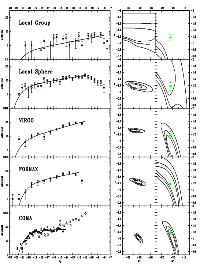
Figure 3: The nearby group and cluster luminosity functions (left) and $1-,2-$ and $3-\sigma$ error ellipses for a Schechter function fit to either the full luminosity range ($-22<M<$ various, middle) or the range comparable to the field range ($-22<M-5\mbox{log}h<-17$, right), all fits are to the solid data points. Local group data: Pritchet & van den Bergh 1999 (solid); Mateo 1998 (open), Local sphere data: Jerjen, Binggeli, Freeman 2000 (solid); Karachtenseva et al 2002 (open), Virgo data: Trentham & Hodgkin 2001 (solid); Fornax data: Ferguson 1989 + Deady et al 2003 (solid); Coma data: Mobasher et al 2003 (solid); Beijersbergen et al 2002 (open triangles), Trentham 1998 (open circles) and Andreon & Culliandre 2002 (open squares). The solid line shows, in each case, the optimal Schechter function fit over the full range of data. The data point and errorbars on the right most panels shows the location of the adopted global luminosity function.

3.1 Coma

The Coma cluster is worth some brief further comment as there have been a number of recent studies with intriguing and even conflicting results. On the largest scale Beijersbergen et al (2002) sample 5.2 sq degrees using background subtraction to determine the overall LF finding an anomalously low $M^{*}$ ($-19.0+5\mbox{log}h_{0.68}$) when compared to the 1 sq degree spectroscopic study of Mobasher et al (2003). Conversely Mobasher et al find a significantly flatter faint-end slope than Beijersbergen et al. More restricted surveys such as Trentham (1998) and Andreon & Culliandre (2002) which focus on the core find evidence for an upturn and/or dip inconsistent with the larger area studies (see Fig. 3). However Beijersbergen et al show that when they confine themselves to the Trentham region they also recover the identical dip and upturn as seen by Trentham. A plausible explanation from a close reading of the relevant papers is the following. Beijersbergen et al may have over estimated their field counts at the bright-end, (see their Table 4 Column 6 which is flatter than the expected $\log\mbox{ndm}\propto 0.6m$ relation at bright mags), this will have minimal impact upon their core LF where the cluster contrast is higher — hence agreement with Trentham — but results in a significant bright-end over-subtraction of the full cluster area — hence disagreement with Mobasher et al. Meanwhile Mobasher et al may suffer from some B-band incompleteness in their R-band selected spectroscopic sample. Finally the Trentham and Andreon & Culliandre LFs are dominated by the core population and the additional structures (LFs dips, upturns) must therefore be core phenomena resulting from strong evolutionary processes in the core region. Clearly the definitive study of Coma remains to be done and represents an excellent opportunity for a space-based survey where high-resolution imaging can be used to determine accurate cluster membership.

4 Composite Cluster LFs

For clusters beyond Coma the majority of studies have relied on the background subtraction of the field galaxy population to recover the cluster luminosity function to comparably faint absolute magnitudes (e.g., Driver et al 1994). As the discussion on Coma above suggests the method of background subtraction, while efficient, is susceptible to a variety of errors. In Driver et al (1998) we discuss the criterion for successful background subtraction in substantial detail. In essence the process is only reliable for very rich clusters where the contrast of the cluster population is high. Valotto, Moore & Lambas (2001) more recently argue for a bias towards steeper faint-end slopes because of preferential alignments between clusters and filaments. While this argument has some merit locally it does not hold for clusters at intermediate redshifts $z>0.1$. The reason for this is that structures are correlated only over scales of order 100Mpc minimising the impact upon clusters at appreciable distances. However Valotto et al do highlight the potential impact of cosmic variance in general and some analysis have neglected to include this significant error component.

Compounding this issue is also the ad hoc coverage of the various studies. In particular the majority of deep studies which have recovered LFs to faint absolute magnitudes sample only the core region identifying features such as dips and upturns similar to that seen in Coma. Overall the conclusions fall into two opposing camps, those that find significant variations between clusters (for example Garilli et al 1999; Goto et al 2002 and qv) and those that do not (for Paolillo et al 2001 and qv). The derived composite LFs for these three surveys are shown in Table 1. So are the variations real or an artifact due to factors such as areal coverage, cosmic variance and/or surface brightness incompleteness between the cluster and reference fields ? Until direct membership is ascertained via either spectroscopy, photometric redshifts or high-resolution space-based imaging it is unlikely that results from background subtraction can be taken as conclusive either way.

Figure 4: The global (solid line) and composition cluster LF (open circles) from within the 2dFGRS survey (left) along with the appropriate errors (right). Once again we find that the field and cluster LFs are in statistical agreement.

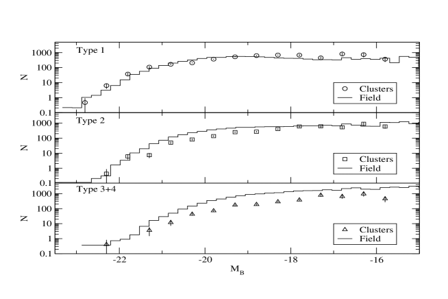
Figure 5: The global (solid lines) and composition cluster LF (open circles) subdivided according to spectral type from early (top) to intermediate (middle) and late (bottom).

5 The 2dFGRS Cluster and Field Luminosity Functions

From the above it is clear that, for the moment, the only reliable way to fully assess the environmental impact on the LF is from within a single large spectroscopically confirmed and self-consistent catalogue. The 2dFGRS offers such an opportunity (see De Propris et al 2003). The 2dFGRS is a magnitude limited redshift survey to an approximate limit of $b_{j}=19.45$ with 221233 redshifts and 92% completeness. The survey has median redshift of $\sim 0.12$ and contains 60 well sampled nearby rich clusters (see De Propris et al. 2002). Full details of the analysis are given in De Propris et al (2003) however Fig. 4 shows the end result comparing the derived field (solid line) and composite cluster (open circles) LFs along with the error ellipses. Note that the field and composite cluster LFs are based upon $\sim 75,000$ and 4,186 spectroscopically confirmed galaxies respectively. The formal Schechter function fits are also shown in Table 1. These suggest a marginally brighter $M^{*}$ and marginally steeper $\alpha$. Perhaps more important though De Propris et al go on to subdivide their sample of 60 clusters according to; rich versus poor, high versus low velocity dispersion, Bautz-Morgan class I,I-II,II versus II-III,III and inner versus outer. In all cases the composite LFs remain consistent with the original composite LF, although it is noted that the composite inner LF is poorly fit by a Schechter function indicating an upturn comparable to that seen in the core Coma studies. Statistically though the only significant variation comes when the field and cluster LFs are subdivided according to type. In these case it is seen that the early-type galaxies have both a slightly brighter and steeper LF while the late-type galaxies remain unchanged in shape but reduced in terms of relative normalisations, see Fig. 5.

6 Conclusions

At face value we must conclude that the galaxy luminosity function appears ubiquitous across all environments studied with only marginal evidence for a slightly brighter $M^{*}$ and a slightly steeper $\alpha$ in clusters (see also the article in these proceedings by Christlein). Only in the very core regions of rich clusters or when the population is sub-divided according to spectral type are significant variations seen. We postulate that these results lead to three likely conclusions:

(1) Cluster infall is an ongoing process with a substantial fraction of the cluster population infalling in recent times. This explains the universality of the LF from the field to rich clusters and constrains any epoch of major merging to have occurred prior to the epoch of cluster formation.

(2) Star-formation is effectively and efficiently inhibited in the infalling population however the halo merger rate is low. This explains the variation with spectral type but not in the overall LF. Hence while galaxies may have shifted their spectral classes their broad-band output remains mostly unchanged.

(3) Dramatic evolutionary processes (merger, harassment etc) resulting in the construction of the cD/D galaxies and destruction of the dwarf population is confined to the core region. This explains the dips and upturns seen in Coma, the 2dFGRS core sample and numerous deep background subtracted core studies.

This is a data rich time for this field with the development of wide field mosaics, the Advanced Camera for Surveys and the upcoming large-format infrared detectors. We look forward to the power of these technologies being brought to bear on this unfolding story.

Table 1: A summary of Schechter LF estimates.

Survey	Limit	$M_{B}^{*}-5\mbox{log}h_{0.68}$	$\alpha$
GLOBAL	$M_{B}\leq-17$	$-20.47\pm 0.2$	$-1.17\pm 0.02$
LOCAL GROUP	$M_{B}\leq-7$	$-21^{+4}_{-2}$	$-1.2^{+0.24}_{-0.14}$
LOCAL SPHERE	$M_{B}\leq-11$	$-20.1^{+1.2}_{-0.6}$	$-1.19^{+0.05}_{-0.06}$
VIRGO	$M_{B}\leq-11$	$-20.2^{+0.7}_{-0.5}$	$-1.32^{+0.03}_{-0.03}$
FORNAX	$M_{B}\leq-12$	$-20.2^{+0.5}_{-0.4}$	$-1.23^{+0.04}_{-0.03}$
COMA	$M_{B}\leq-14$	$-20.1^{+0.25}_{-0.20}$	$-1.01^{+0.04}_{-0.05}$
Garilli et al1	$M_{B}\leq-17$	$-20.6\pm 0.1$	$-0.97^{+0.04}_{-0.02}$
Paolillo et al1	$M_{B}\leq-16$	$-20.5^{+0.13}_{-0.17}$	$-1.07^{+0.09}_{-0.07}$
Goto et al1	$M_{B}\leq-16.5$	$-21.47\pm 0.11$	$-1.00\pm 0.06$
2dFGRS FIELD	$M_{B}\leq-17$	$-20.35\pm 0.04$	$-1.19\pm 0.01$
2dFGRS CLUSTER	$M_{B}\leq-17$	$-20.62\pm 0.07$	$-1.28\pm 0.03$

¹ $g$-band data converted to $B$ assuming $B=g+0.54$

- [1]
- Andreon & Culliandre (2001) Andreon, S., Culliandre, J.-C., 2002, ApJ, 569, 144
- Beijersbergen et al (2002) Beijersbergen, M., Hoekstra, H., van Dokkum, P.G., & van der Hulst, T., 2002, MNRAS, 329, 385
- Blanton et al (2001) Blanton, M., et al 2001, AJ, 121, 2358
- Blanton et al (2003) Blanton, M., et al 2003, ApJ, in press
- Brown et al (2001) Brown, W.R., Geller, M.J., Fabricant, D.G., Kurtz, M.J., 2001, AJ, 122, 714
- Colless et al (2001) Colless, M.M., et al 2001, MNRAS, 328, 1039
- Cross & Driver (2002) Cross, N.J.G., Driver, S.P., 2002, MNRAS, 329, 579
- Deady et al (2003) Deady, J.H., et al 2002, MNRAS, 336, 851
- De Propris et al (2002) De Propris, R., et al 2002, MNRAS, 329, 87
- Driver (1999) Driver, S.P., 1999, ApJ, 526, 69
- Driver et al (1999) Driver, S.P., Couch W.J., Phillipps S., Smith, R.M., 1998, 301, 357
- Driver et al (1994) Driver, S.P., et al., 1994, MNRAS, 268, 393
- Ferguson, H., (1989) Ferguson, H., 1989, AJ, 98, 367
- Garilli et al (1999) Garilli, B.M., Maccagno, D., Andreon S., 1999, A&A, 342, 408
- Goto et al (2002) Goto , T., et al 2002, PASJ, 54, 515
- Jerjen, Binggeli & Freeman (2000) Jerjen, H. Binggeli, B., Freeman, K.C., 2000, ApJ, 119, 593
- Karachentsev et al (2002) Karachentsev, I.D., et al 2002, A&A, 389, 812
- Liske et al (2003) Liske, J., Lemon, D., Driver, S.P., Cross, N.J.G., Couch. W.J., 2003, MNRAS, in press
- Loveday et al (1992) Loveday, J., Peterson B. A., Efstathiou, G., Maddox, S. J. 1992, ApJ, 390, 338
- Marinoni et al (1999) Marinoni, C., Monaco, P., Giruricin, G., Costantini, B., 1999, ApJ, 521, 50
- Marzke et al (1998) Marzke, R., Da Costa, N., Pelligrini, P., Willmer, C., Geller M. 1998, ApJ, 503, 617
- Mateo (1998) Mateo, M., 1998, ARA&A, 36, 435
- Metcalfe et al (1995) Metcalfe, N., Fong, D., Shanks, T., 1995, MNRAS, 274, 769
- Mobasher et al (2003) Mobasher, B., et al., 2003, MNRAS, submitted
- Norberg et al (2002) Norberg, P., et al 2002, MNRAS, in press
- Paolillo et al (2002) Paolillo, M., et al, 2002, A&A, 367, 59
- Phillipps & Disney (1985) Phillipps, S., & Disney, M.J., 1985, A&A, 148, 234
- Press and Schechter (1974) Press, W., Schechter, P.J., 1974, ApJ, 187, 425
- Pritchet & van denBergh (1999) Pritchet, C., van den Bergh, S., 1999, AJ, 118, 883
- Roche & Eales (1999) Roche, N., Eales, S., 1999, MNRAS, 307, 703
- Schechter (1976) Schechter, P.J., 1976, ApJ, 203, 297
- Trentham (1998) Trentham, N., 1998, MNRAS, 294, 193
- Trentham & Hodgkin (2002) Trentham, N., Hodgkin, S., 2002, MNRAS, 333, 423
- Valotto, Moore & Lambas (2001) Valotto, C.A., Moore, B., Lambas, D.G., 2001, ApJ, 546, 157
- Zucca et al (1997) Zucca, E., et al 1997, A&A, 326, 477