Stability of an Ultra-Relativistic Blast Wave in an External Medium with a Steep Power-Law Density Profile

Abstract

We examine the stability of self-similar solutions for an accelerating relativistic blast wave which is generated by a point explosion in an external medium with a steep radial density profile of a power-law index $>4.134$. These accelerating solutions apply, for example, to the breakout of a gamma-ray burst outflow from the boundary of a massive star, as assumed in the popular collapsar model. We show that short wavelength perturbations may grow but only by a modest factor $\lesssim 10$.

PACS numbers: 47.40.Nm, 47.75.+f, 95.30.Lz

I Introduction

The self-similar solutions of relativistic blast waves are of much interest because of their recent applications to the study of Gamma-Ray Bursts (GRBs). A sudden release of a large amount of energy within a small volume results in a strong explosion that drives a relativistic shock into the surrounding medium. At late times the blast wave approaches a self-similar phase whereby its speed and the distribution of the pressure, density, and velocity of the gas behind the shock front do not depend on the length and time scales of the initial explosion, but only on the explosion energy and the properties of the unshocked external medium. The self-similar solutions describing this phase have been first studied by Blandford and McKee [1] (hereafter, BMK). We list their central results, which are relevant to this paper, in section §II.A. Note that in the BMK solution the total energy released in the explosion $E$ is the only relevant parameter.

The BMK solution is only valid for $k<4$, where $k$ is the power-law index of the radial density profile of the external medium, i.e., $\rho_{1}\propto r^{-k}$. When $k\geq 4$, the similarity variable defined by Blandford and McKee [1] is no longer appropriate. Even in the range $3\leq k<4$, the validity of the BMK solution is not justified, because the mass contained behind the shock front diverges if the density profile of the shocked fluid is described by the BMK solution.

The self-similar solutions for steep density profiles with a power-law index $k\geq 4$ were derived recently by Best & Sari [2]. The derivation of these solutions is similar to that in the non-relativistic regime. The self-similar solutions to a non-relativistic blast wave were discovered independently by Sedov [4] , Von Neumann [5], and Taylor [6]. The so-called ”Sedov-Von Neumann-Taylor blast wave” solutions exist only for $k<5$, but Waxman & Shvarts [7] showed that in the range $3\leq k<5$ these solutions fail to describe the asymptotic flow because the energy diverges; instead they found second-type self-similar solutions for $3<k<5$ as well as for $k\geq 5$. The new class of non-relativistic, self-similar solutions describe the flow in a limited spatial region $D(t)\leq r\leq R(t)$, where $R(t)$ is the shock radius and $D(t)$ coincides with a $C_{+}$ characteristic so that the flow inside the region $r<D(t)$ does not affect the flow in the outer self-similar region. The self-similar solution has to cross the sonic line into the region where the $C_{+}$ characteristic can not catch-up with the shock front. The solution describes a shock accelerating with a temporal dependence whose power-law index is uniquely determined by requiring that the self-similar solution cross the sonic line at a singular point. Note that in these second-type self-similar solutions the total energy released in the explosion $E$ is not a relevant parameter. Although the energy in the self-similar part of the flow approaches a constant as time diverges, the fraction of the explosion energy $E$ carried by the self-similar component depends on the details of the initial conditions. Thus, contrary to the BMK case, dimensional arguments can not be used to determine the power-law index of the temporal dependence. Instead, the singular point determines the temporal power-law index. In the ultra-relativistic regime, the second-type self-similar solutions for $k\geq 4$ can similarly be obtained by requiring that they cross the sonic line at a singular point. Best & Sari [2] found that these self-similar solutions exist for $k>5-\sqrt{3/4}$ and describe accelerating shock waves. However, the properties of the flow in the self-similar region, such as the energy and mass contained in the region, were not discussed.

In this paper, we rederive the self-similar solutions of ultra-relativistic blast waves for $k>4$ using a different self-similar variable and discuss the properties of the flow in the self-similar regime. Our main goal is to study the stability of these self-similar solutions. The stability of the Waxman-Shvarts self-similar solutions in the non-relativistic regime was studied by Sari, Waxman & Shvarts [8]. They found that shocks accelerating at a rate larger than a critical value and corresponding to solutions that diverge in finite time, are unstable for small and intermediate wavenumbers. Shocks that accelerate at a rate smaller than the critical rate are stable for most wavenumbers. The acceleration rate can be quantified by the measure $\delta=R\ddot{R}/\dot{R}^{2}$, where the dots denote time derivatives and $R(t)$ is the radius of the shock front. This measure provides the fractional change of the velocity over a characteristic time scale for evolution ($R/\dot{R}$). Solutions that diverge in finite time have $\delta>1$ while others have $\delta<1$. Thus, when shocks accelerate sufficiently fast they become unstable.

In the following sections we study the stability of the self-similar solutions of ultra-relativistic blast waves for steep density profiles with a power-law index $k>4$. The self-similar solutions are described in §II. We list the BMK solutions for $k<4$ in §II.A and derive the self-similar solutions for $k>4$ in §II.B. In §III, we discuss the properties of the self-similar flow and calculate the energy and mass contained in the self-similar regime. In §IV and §V, we study the stability of the self-similar solutions. Finally, we summarize our main results in §VI.

II Self-Similar Solutions

A BMK solutions for $k<4$

For pedagogical reasons, we first briefly outline the derivation of the self-similar solutions of relativistic blast waves for $k<4$ by Blandford & McKee. For a complete derivation, the reader is referred to the original paper [1].

Assuming an ultra-relativistic equation of state, $p=(1/3)e$, where $p$ and $e$ are the pressure and energy density measured in the fluid frame, the equations describing a relativistic, spherically-symmetric, perfect fluid can be written as,

$$\frac{d}{dt}(p\gamma^{4})=\gamma^{2}\frac{\partial p}{\partial t},$$ (1)

$$\frac{d}{dt}\ln(p^{3}\gamma^{4})=-\frac{4}{r^{2}}\frac{\partial}{\partial r}(r^{2}\beta),$$ (2)

$$\frac{\partial n^{\prime}}{\partial t}+\frac{1}{r^{2}}\frac{\partial}{\partial r}(r^{2}n^{\prime}\beta)=0,$$ (3)

where $n^{\prime}$ is the density as measured in the laboratory frame, $\gamma$ and $\beta$ are the Lorentz factor and velocity of the fluid, and

$$\frac{d}{dt}\equiv\frac{\partial}{\partial t}+\beta\frac{\partial}{\partial r}$$ (4)

is the convective derivative. Throughout this paper we set the speed of light $c$ to unity. Assuming that the blast wave is ultra-relativistic so that the Lorentz factor of the shock front $\Gamma$ and the shocked fluid $\gamma$ are much larger than unity, we only search for solutions accurate to the lowest order in $\gamma^{-2}$ and $\Gamma^{-2}$.

The effective thickness of the blast wave is approximately $R/\Gamma^{2}$, where $R$ is the radius of the shock front. Thus an appropriate choice of similarity variable is

$$\xi=\left(1-\frac{r}{R}\right)\Gamma^{2}\geq 0.$$ (5)

Next we assume that the external medium has a scale-free, power-law density profile $\rho_{1}\propto r^{-k}$. Ignoring radiative losses, the total energy contained in the shocked fluid remains constant and so the Lorentz factor of the shock front evolves adiabatically as a power law,

$$\Gamma^{2}\propto t^{-m},\ \ m>-1.$$ (6)

Keeping only terms up to order $O(\Gamma^{-2}t)$, the shock radius is then given by

$$R=t\left[1-\frac{1}{2(m+1)\Gamma^{2}}\right].$$ (7)

A more convenient similarity variable can be defined as

$$\chi=1+2(m+1)\xi=[1+2(m+1)\Gamma^{2}]\left(1-\frac{r}{t}\right).$$ (8)

In terms of $\chi$, the pressure, velocity, and density in the shocked fluid can be written as

$$p=\frac{2}{3}w_{1}\Gamma^{2}f(\chi),$$ (9)

$$\gamma^{2}=\frac{1}{2}\Gamma^{2}g(\chi),$$ (10)

$$n^{\prime}=2n_{1}\Gamma^{2}h(\chi),$$ (11)

where $\chi\geq 1$, $w_{1}$ and $n_{1}$ are the enthalpy and number density of the unshocked external medium. We assume that the unskocked external medium is cold, so that $w_{1}$ equals the energy density $\rho_{1}$. The jump conditions for a strong ultra-relativistic shock are satisfied by the boundary conditions

$$f(1)=g(1)=h(1)=1.$$ (12)

For an adiabatic impulsive blast wave, equations (1)–(3) admit a simple analytical solution, first derived by BMK [1]

$$f=\chi^{-(17-4k)/(12-3k)},$$ (13)

$$g=\chi^{-1},$$ (14)

$$h=\chi^{-(7-2k)/(4-k)},$$ (15)

for

$$m=3-k>-1.$$ (16)

B Self-similar solutions for $k>4$

In searching for self-similar solutions for $k>4$, we assume that the Lorentz factor of the shock front still obeys a power law, $\Gamma^{2}\propto t^{-m}$ with $m<-1$. When $m<-1$, the similarity variable $\chi$ defined in equation (8) (and used by Best & Sari [2]) could be negative. For convenience we will use $\xi$, defined in equation (5), instead as our similarity variable. If at an initial time $t_{0}$, the shock radius is $R_{0}$ and the Lorentz factor of the shock front is $\Gamma_{0}$, then at a later time $t$, to $O(\Gamma^{-2}t)$ the shock radius is given by

$$R=R_{0}+t\left[1-\frac{1}{2(m+1)\Gamma^{2}}\right]-t_{0}\left[1-\frac{1}{2(m+1)\Gamma_{0}^{2}}\right].$$ (17)

We can rewrite this equation as

$$R=t\left[1-\frac{1}{2(m+1)\Gamma^{2}}\right]+a,$$ (18)

where $a$ is a constant dictated by the initial conditions. This equation for $R$ with $m<-1$ differs from equation (7) by a constant $a$. However, we can choose the initial time $t_{0}$ such that $a$ is equal to zero. This is appropriate because of two reasons. First, the self-similar solutions are valid at much later times $t>>t_{0}$, thus the effect of the special choice of $t_{0}$ can be ignored. Second, what matters in the derivation of the self-similar solutions is the derivative of $R$, instead of $R$ itself. When $a=0$, the similarity variable becomes

$$\xi=\left(1-\frac{r}{R}\right)\Gamma^{2}=\Gamma^{2}-\frac{r}{t}\left[\Gamma^{2}+\frac{1}{2(m+1)}\right].$$ (19)

Note that we have ignored higher order terms in $\Gamma^{-2}$ in the above expression.

Similarly to equations (9)–(11), we write the pressure, velocity, and density in the shocked fluid as

$$p=\frac{2}{3}w_{1}\Gamma^{2}f(\xi),$$ (20)

$$\gamma^{2}=\frac{1}{2}\Gamma^{2}g(\xi),$$ (21)

$$n^{\prime}=2n_{1}\Gamma^{2}h(\xi),$$ (22)

where $\xi\geq 0$ and the boundary conditions,

$$f(0)=g(0)=h(0)=1,$$ (23)

correspond to the jump conditions for a strong ultra-relativistic shock.

We can now treat $\Gamma^{2}$ and $\xi$ as two new independent variables in place of $r$ and $t$, and get

$$t\frac{\partial}{\partial t}=-m\Gamma^{2}\frac{\partial}{\partial\Gamma^{2}}+\left[\Gamma^{2}-\frac{1}{2}\frac{m}{m+1}-(m+1)\xi\right]\frac{\partial}{\partial\xi},$$ (24)

$$t\frac{\partial}{\partial r}=-\left[\Gamma^{2}+\frac{1}{2(m+1)}\right]\frac{\partial}{\partial\xi},$$ (25)

$$t\frac{d}{dt}=-m\Gamma^{2}\frac{\partial}{\partial\Gamma^{2}}-\left[\frac{1}{2}+(m+1)\xi-\frac{1}{g}\right]\frac{\partial}{\partial\xi}.$$ (26)

In deriving the above equations, we have assumed that the blast wave is ultra-relativistic so that $\Gamma>>1$ and $\gamma>>1$. Thus we only keep terms of the lowest contribution order in $\Gamma^{-2}$ and $\gamma^{-2}$.

Substituting equations (24)–(26) into equations (1)–(3), we obtain the following differential equations for $f$, $g$, and $h$:

$$2(3m+k)g+[g+2(m+1)g\xi+2]\frac{1}{f}\frac{df}{d\xi}$$ (27)

$$+2[g+2(m+1)g\xi-2]\frac{1}{g}\frac{dg}{d\xi}=0,$$ (28)

$$2(5m+3k-8)g+3[g+2(m+1)g\xi-2]\frac{1}{f}\frac{df}{d\xi}$$ (29)

$$+2[g+2(m+1)g\xi+2]\frac{1}{g}\frac{dg}{d\xi}=0,$$ (30)

$$2(m+k-2)g+[g+2(m+1)g\xi-2]\frac{1}{h}\frac{dh}{d\xi}$$ (31)

$$+2\frac{1}{g}\frac{dg}{d\xi}=0.$$ (32)

Using a new variable,

$$y=[1+2(m+1)\xi]g,$$ (33)

we rewrite equations (28)–(32) as follows

$$\frac{1}{g}\left(\frac{1}{f}\frac{df}{d\xi}\right)=\frac{2[4(2m+k-2)-(m+k-4)y]}{y^{2}-8y+4},$$ (34)

$$\frac{1}{g}\left(\frac{1}{g}\frac{dg}{d\xi}\right)=\frac{2[(7m+3k-4)-(m+2)y]}{y^{2}-8y+4}.$$ (35)

$$\frac{1}{g} \left(\frac{1}{h}\frac{dh}{d\xi}\right)=-2[(y^{2}-8y+4)(y-2)]^{-1}$$ (36)

$$\times[(m+k-2)y^{2}-(10m+8k-12)y$$ (37)

$$+(18m+10k-16)].$$ (38)

One solution to the above equations is obtained for $y=1$ and $m=3-k$, and corresponds to the BMK solution. From the definition of $y$, $y=[1+2(m+1)\xi]g$, and the requirement that $g$ be positive it follows that this solution is only valid for $m>-1$, i.e., $k<4$.

In our search for possible solutions with $k>4$, we start by analyzing equations (34)–(38). The right-hand-side of these equations diverges to infinity if $y^{2}-8y+4=0$. This corresponds to two singular points, $y_{1}=4-2\sqrt{3}=0.536$ and $y_{2}=4+2\sqrt{3}=7.464$. In addition, equation (38) has another singular point at $y_{3}=2$. The solution to equation (34) can bypass the singular points $y_{1}$ and $y_{2}$ if the numerator on the right-hand-side of the equation vanishes at $y_{1}$ or $y_{2}$. This gives

$$m_{1,2}=\frac{8-4k+(k-4)y_{1,2}}{8-y_{1,2}}.$$ (39)

It is easy to prove that when $m=m_{1}$, equations (35) and (38) will also bypass the singular point $y_{1}$ (the numerator in the right hand side of each equation is equal to zero at $y_{1}$). The same is true for $m=m_{2}$ and the singular point $y_{2}$. We will show below that when $m=m_{1}$ and $k$ is bigger than a critical value $k_{c}$, we have $y\leq 1$, thus equations (34)–(38) are able to bypass the singular point $y_{1}$ and never reach $y_{2}$ and $y_{3}$. The critical value $k_{c}$ can be calculated by setting $m_{1}$ equal to $3-k$, the $m$ value corresponding to a BMK solution. For $y_{1}=4-2\sqrt{3}$, we get

$$m_{1}=12\sqrt{3}-20+(3-2\sqrt{3})k.$$ (40)

Thus $m_{1}=3-k$ gives us

$$k_{c}=5-\frac{\sqrt{3}}{2}=4.134$$ (41)

The value of $m_{1}$ corresponding to $k_{c}$ is $m_{1c}=-2+\sqrt{3}/2=-1.134$. Thus when $k>k_{c}$, we have $m_{1}<m_{1c}$.

We now prove that when $m=m_{1}$ and $k>k_{c}$, we always have $y\leq 1$. Using equation (35) and the definition of $y$ in equation (33) we obtain

$$\frac{dy}{d\xi} = 2(m+1)g(\xi)+\frac{y}{g(\xi)}\frac{dg}{d\xi}$$ (42)

$$= -\frac{2g(\xi)[y^{2}+(m-3k+12)y-4(m+1)]}{y^{2}-8y+4}.$$ (43)

When $m=m_{1}$, the above equation can be rewritten as

$$\frac{dy}{d\xi}=-\frac{2g(y-b)}{y-y_{2}},$$ (44)

where

$$b=4-10\sqrt{3}+2\sqrt{3}k=1+2\sqrt{3}(k-k_{c}).$$ (45)

When $k>k_{c}$, we have $b>1$. We also have $g>0$ and $y_{2}=4+2\sqrt{3}>1$, and so the right hand side of equation (44) is negative when $y\leq 1$. Since the boundary condition is $y(\xi=0)=1$, $y(\xi)$ must be a monotonically decreasing function of $\xi$ with $y(\xi)\leq 1$. The asymptotic behavior of $y(\xi)$ can be derived as follows. When $\xi$ is large, $y$ is negative and $|y|$ is large so that equation (44) can be approximated as

$$\frac{dy}{d\xi}\simeq-2g\simeq-\frac{1}{m_{1}+1}\frac{y}{\xi},$$ (46)

where we have used the approximation $y\simeq 2(m_{1}+1)\xi g$ for large $\xi$. Equation (46) yields

$$-y\propto\xi^{-1/(m_{1}+1)}.$$ (47)

Note that when $k>k_{c}$, we have $m_{1}<m_{1c}<-1$. Thus the exponent in the above power law is always positive.

It can be proven that when $k\leq k_{c}$, equations (34)–(38) can not bypass all the singular points with either $m_{1}$ or $m_{2}$, and so the BMK solution is the only possible solution. When $k>k_{c}$, the equations can not bypass all the singular points with $m_{2}$. But this by itself is not sufficient for justifying that $m_{1}$ is the only viable choice. What if the solutions cut-off at some radius before reaching any singular points? We know that in order not to run into divergences of the energy or mass of the system, the solutions must be truncated at some radius $r_{+}$ (or $\xi_{+}$ in terms of the similarity variable), which should coincide with a $C_{+}$ characteristic line. The $C_{+}$ characteristic guarantees that the flow in the inner region $r<r_{+}$ will not influence the flow in the self-similar region $r_{+}\leq r\leq R$. This $C_{+}$ characteristic should not overtake the shock front in finite time, otherwise the self-similar region will eventually disappear. This argument has been applied in the non-relativistic case [7]. We will prove below that in order to get to the regime where the $C_{+}$ characteristics can not catch the shock front, the solutions have to pass the singular point $y_{1}$, making $m_{1}$ the only viable choice.

First, let us derive the equation for a $C_{+}$ characteristic. We use $v$ to denote the fluid velocity in the laboratory frame. The sound speed in the fluid frame is $u^{\prime}_{s}=1/\sqrt{3}$. Thus the sound speed in the laboratory frame $u_{s}$ is given by

$$u_{s} = \frac{u^{\prime}_{s}+v}{1+vu^{\prime}_{s}}=1-\frac{\sqrt{3}-1}{\sqrt{3}+1}\frac{1}{2\gamma^{2}}$$ (48)

$$= 1-\frac{\sqrt{3}-1}{\sqrt{3}+1}\frac{1}{\Gamma^{2}g(\xi)},$$ (49)

where we only keep the first-order term in $\gamma^{-2}$. Thus, a $C_{+}$ characteristic is described by

$$\frac{dr_{+}}{dt}=1-\frac{\sqrt{3}-1}{\sqrt{3}+1}\frac{1}{\Gamma^{2}g(\xi_{+})}.$$ (50)

We can rewrite this equation in terms of the similarity variable $\xi_{+}$. Using the definition of $\xi$ in equation (5), and the relations, $dR/dt=1-1/(2\Gamma^{2})$, $d\Gamma^{2}/dt=-m\Gamma^{2}/t$, we obtain

$$\frac{dr}{dt}=1-\frac{1}{2\Gamma^{2}}-\frac{(m+1)}{\Gamma^{2}}\xi-\frac{t}{\Gamma^{2}}\frac{d\xi}{dt},$$ (51)

where we only keep the first-order term in $\Gamma^{-2}$. Substituting equation (51) into equation (50), we get

$$t\frac{d\xi_{+}}{dt}=\frac{\sqrt{3}-1}{\sqrt{3}+1}\frac{1}{g(\xi_{+})}-(m+1)\xi_{+}-\frac{1}{2},$$ (52)

which describes the evolution of a $C_{+}$ characteristic. We can further rewrite this equation as

$$t\frac{d\xi_{+}}{dt}=-\frac{1}{2g(\xi_{+})}(y_{+}-y_{1}),$$ (53)

where

$$y_{+}=[1+2(m+1)\xi_{+}]g(\xi_{+}).$$ (54)

Equation (53) implies that when $y_{+}>y_{1}$, the right-hand-side of the equation is negative and so $\xi_{+}$ will decrease with time and the $C_{+}$ characteristic will approach the shock front. Only when $y_{+}<y_{1}$, $\xi_{+}$ will increase with time and the $C_{+}$ characteristic will not overtake the shock front. Also notice that the self-similar solution has the boundary condition $y(\xi=0)=1>y_{1}$. We thus proved that in order to get to the regime where $C_{+}$ characteristics can not overtake the shock front, the self-similar solution must pass through the singular point $y_{1}$, and therefore $m_{1}$ is the only viable choice.

We can now attempt to obtain the self-similar solutions for equations (34)–(38). For $m=m_{1}$, these equations become

$$\frac{1}{g}\left(\frac{1}{f}\frac{df}{d\xi}\right)=-\frac{2(m_{1}+k-4)}{y-y_{2}},$$ (55)

$$\frac{1}{g}\left(\frac{1}{g}\frac{dg}{d\xi}\right)=-\frac{2(m_{1}+2)}{y-y_{2}},$$ (56)

$$\frac{1}{g}\left(\frac{1}{h}\frac{dh}{d\xi}\right)=-\frac{2(m_{1}+k-2)(y-d)}{(y-y_{2})(y-2)},$$ (57)

where

$$d=4+\sqrt{3}+\frac{3+2\sqrt{3}}{k+\sqrt{3}-4}.$$ (58)

Treating $y$ as the independent variable instead of $\xi$ and making use of equation (44), equations (55)–(57) can be rewritten as

$$\frac{1}{f}\frac{df}{dy}=\frac{m_{1}+k-4}{y-b},$$ (59)

$$\frac{1}{g}\frac{dg}{dy}=\frac{m_{1}+2}{y-b},$$ (60)

$$\frac{1}{h}\frac{dh}{dy}=\frac{(m_{1}+k-2)(y-d)}{(y-2)(y-b)}.$$ (61)

The boundary conditions are $f(y=1)=g(y=1)=h(y=1)=1$. Equations (59) and (60) have the solutions

$$f=\left(\frac{b-y}{b-1}\right)^{m_{1}+k-4},$$ (62)

$$g=\left(\frac{b-y}{b-1}\right)^{m_{1}+2}.$$ (63)

A special case is obtained at $k=6$ ($m_{1}=-2$) for which $f(y)=g(y)=1$. When $b\neq 2$ ($k\neq(15-\sqrt{3})/3$), equation (61) has the solution

$$h=\left[\left(\frac{1}{2-y}\right)^{d-2}\left(\frac{b-y}{b-1}\right)^{d-b}\right]^{(m_{1}+k-2)/(2-b)}.$$ (64)

When $b=2$ ($k=(15-\sqrt{3})/3$), equation (61) has the solution

$$h = (2-y)^{m_{1}+k-2}$$ (66)

$$\times\exp\left[(m_{1}+k-2)(d-2)\left(\frac{1}{2-y}-1\right)\right].$$

In general, the functions $f(\xi)$, $g(\xi)$ and $h(\xi)$ do not admit simple analytical forms. Their values can be derived numerically from equations (62)–(66). For example, $g(\xi)$ satisfies the implicit algebraic equation

$$g(\xi)=\left(\frac{b-[1+2(m_{1}+1)\xi]g(\xi)}{b-1}\right)^{m_{1}+2}.$$ (67)

But generally, we can derive the analytical forms for the asymptotic behaviors of $f(\xi)$, $g(\xi)$ and $h(\xi)$ in the limit of large $\xi$. In this limit, $y$ is negative and $|y|$ is large, and so equation (63) yields

$$g\simeq\left(\frac{-y}{b-1}\right)^{m_{1}+2}\simeq\left[\frac{-2(m_{1}+1)\xi g}{b-1}\right]^{m_{1}+2}.$$ (68)

We can solve $g(\xi)$ from the above equation and get

$$g(\xi)\simeq\alpha_{g}\xi^{-(m_{1}+2)/(m_{1}+1)},$$ (69)

where

$$\alpha_{g}=\left[\frac{-2(m_{1}+1)}{b-1}\right]^{-(m_{1}+2)/(m_{1}+1)}.$$ (70)

Using equation (69) we obtain the asymptotic form of $y(\xi)$ for large $\xi$

$$y(\xi)\simeq-\alpha_{y}\xi^{-1/(m_{1}+1)},$$ (71)

where

$$\alpha_{y}=\left[\frac{-2(m_{1}+1)}{(b-1)^{m_{1}+2}}\right]^{-1/(m_{1}+1)}.$$ (72)

Using equation (71), we can derive the asymptotic form of $f(\xi)$ for large $\xi$ from equation (62) and get

$$f(\xi)\simeq\alpha_{f}\xi^{-(m_{1}+k-4)/(m_{1}+1)},$$ (73)

where

$$\alpha_{f}=\left[\frac{-2(m_{1}+1)}{b-1}\right]^{-(m_{1}+k-4)/(m_{1}+1)}.$$ (74)

Similarly, the asymptotic form of $h(\xi)$ for large $\xi$ can be derived from equations (64) and (66). We obtain

$$h(\xi)\simeq\alpha_{h}\xi^{-(m_{1}+k-2)/(m_{1}+1)},$$ (75)

where

$$\alpha_{h}=\left[\frac{-2(m_{1}+1)}{1-(b-1)^{(m_{1}+1)(d-2)/(2-b)}}\right]^{-(m_{1}+k-2)/(m_{1}+1)}$$ (76)

if $b\neq 2$, and

$$\alpha_{h} = \left[\frac{-2(m_{1}+1)}{(b-1)^{m_{1}+2}}\right]^{-(m_{1}+k-2)/(m_{1}+1)}$$ (78)

$$\times\exp[-(m_{1}+k-2)(d-2)]$$

if $b=2$.

Equation (53), which describes the evolution of the $C_{+}$ characteristic, can also be rewritten using the variable $y$. Using equation (44), we obtain

$$t\frac{dy_{+}}{dt}=\frac{(y_{+}-y_{1})(y_{+}-b)}{y_{+}-y_{2}}.$$ (79)

We have proven earlier that when $k>k_{c}$ one finds $b>1$ and $y\leq 1$. Thus the sign of the right-hand-side of the above equation is decided by the term $(y_{+}-y_{1})$. If a $C_{+}$ characteristic emerges from the region $y<y_{1}$, i.e., $y_{+}(t=t_{0})<y_{1}$, we know that $y_{+}(t)$ will decrease with time or equivalently $\xi_{+}(t)$ will increase with time and the $C_{+}$ characteristic will not catch-up with the shock front.

Equations (55)–(57) can also be solved numerically for different values of $k$. We plot the results for $k=5.5$ ($m_{1}=-1.77$) and $k=6.5$ ($m_{1}=-2.23$) in Figure 1. When $k_{c}<k<6$, the function $f(\xi)$ decreases with increasing $\xi$ while the function $g(\xi)$ increases with increasing $\xi$. This implies that when moving inwards away from the shock front, the pressure decreases while the Lorentz factor increases. For $k>6$ the situation is reversed. For all $k>k_{c}$, the function $h(\xi)$ increases with $\xi$ implying that the density always increases when moving inwards away from the shock front.

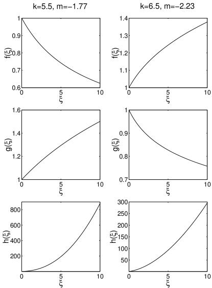
FIG. 1.: Distributions of the self-similar functions $f(\xi)$, $g(\xi)$ and $h(\xi)$. The left column corresponds to $k=5.5$ and $m_{1}=-1.77$, while the right column corresponds to $k=6.5$ and $m_{1}=-2.23$.

III Properties of the flow in the self-similar region

We now examine the properties of the flow in the self-similar region bounded by $\xi=0$ and $\xi=\xi_{+}(t)$, where $\xi_{+}(t)$ coincides with a $C_{+}$ characteristic that emerges from the region $y<y_{1}$. The evolution of the $C_{+}$ characteristic is described by equation (79) with the initial condition $\xi_{+}(t=t_{0})=\xi_{0}$, and correspondingly $y_{+}(t=t_{0})=y_{0}<y_{1}$. By solving equation (79), we get the following equation for $y_{+}(t)$,

$$\left(\frac{y_{1}-y_{+}}{y_{1}-y_{0}}\right)^{(y_{2}-y_{1})/(b-y_{1})}\left(\frac{b-y_{+}}{b-y_{0}}\right)^{(b-y_{2})/(b-y_{1})}=\frac{t}{t_{0}}.$$ (80)

We can now derive the asymptotic behavior of the $C_{+}$ characteristic at $t\rightarrow\infty$. In this limit $|y_{+}(t)|$ is large, and equation (80) yields

$$y_{+}(t)\simeq-\alpha_{0}t,$$ (81)

where

$$\alpha_{0}=(y_{1}-y_{0})^{(y_{2}-y_{1})/(b-y_{1})}(b-y_{0})^{(b-y_{2})/(b-y_{1})}/t_{0}.$$ (82)

Substituting equation (71) into equation (81), we get

$$\xi_{+}(t)\simeq\alpha_{+}t^{-(m_{1}+1)},$$ (83)

where

$$\alpha_{+}=\left(\frac{\alpha_{0}}{\alpha_{y}}\right)^{-(m_{1}+1)}.$$ (84)

The initial condition for the $C_{+}$ characteristic, namely the value of the $C_{+}$ characteristic with which $\xi_{+}(t)$ coincides, contains the information about the initial explosion.

The shock front is accelerating with a power-law temporal dependence of its Lorentz factor, $\Gamma^{2}\propto t^{-m_{1}}$. How does the $C_{+}$ characteristic propagate? From equations (69) and (83) we find that when $t\rightarrow\infty$,

$$\gamma^{2}(\xi_{+})=\frac{1}{2}\Gamma^{2}g(\xi_{+})\propto t^{2}.$$ (85)

We see that irrespective of the value of $k$, the $C_{+}$ characteristic always accelerates as $\gamma^{2}\propto t^{2}$. We can also calculate the thickness of the self-similar region. Using equations (5) and (83) we obtain when $t\rightarrow\infty$,

$$R-r_{+}=\frac{R\xi_{+}}{\Gamma^{2}}\longrightarrow{\rm const}.$$ (86)

Note that when $-2<m_{1}<m_{1c}$, the $C_{+}$ characteristic accelerates faster than the shock front, but because the Lorentz factors of both surfaces are accelerating as power-laws of time, the $C_{+}$ characteristic can never catch-up with the shock front. Instead, the distance between the two surfaces approaches a constant value at late times.

We can now examine the energy and mass contained in the self-similar region. The energy contained in the spherical shell between $\xi=0$ and $\xi=\xi_{+}(t)$ is given by

$$E=\int_{r_{+}}^{R}16\pi p\gamma^{2}r^{2}dr=\frac{16\pi}{3}w_{1}\Gamma^{2}R^{3}\int_{0}^{\xi_{+}}f(\xi)g(\xi)d\xi.$$ (87)

Using equations (73) and (69), we can calculate the above integral for large values of $\xi_{+}$. This gives,

$$E \simeq \frac{16\pi}{3}\left(-\frac{m_{1}+1}{m_{1}+k-3}\right)\alpha_{f}\alpha_{g}w_{1}\Gamma^{2}R^{3}$$ (89)

$$\times\xi_{+}^{-(m_{1}+k-3)/(m_{1}+1)}.$$

In deriving the above result we have used the fact that when $k>k_{c}$, we have $m_{1}+k-3>0$ and $m_{1}+1<0$, so that the exponent of $\xi_{+}$ in the above equation $-(m_{1}+k-3)/(m_{1}+1)$ is positive. When $t\rightarrow\infty$, $\xi_{+}$ is given by equation (83). In addition $\Gamma^{2}\propto t^{-m_{1}}$, $w_{1}=\rho_{1}\propto R^{-k}$. Thus when $t\rightarrow\infty$,

$$E\longrightarrow{\rm const}.$$ (90)

The total number of particles contained between $\xi=0$ and $\xi=\xi_{+}(t)$ is given by

$$N=\int_{r_{+}}^{R}n^{\prime}4\pi r^{2}dr=8\pi n_{1}R^{3}\int_{0}^{\xi_{+}}h(\xi)d\xi.$$ (91)

Using equations (75) and (83), we obtain that for $t\rightarrow\infty$,

$$N \simeq 8\pi\left(-\frac{m_{1}+1}{k-3}\right)\alpha_{h}n_{1}R^{3}\xi_{+}^{-(k-3)/(m_{1}+1)}$$ (93)

$$\longrightarrow{\rm const}.$$

We have thus proven that both the energy and mass contained between the $C_{+}$ characteristic and the shock front will approach constant values as $t\rightarrow\infty$. The situation is similar to the non-relativistic case [7].

IV Approximate (Analytic) Stability Analysis

In order to analyze the stability of the self-similar solutions obtained in §II.B, we first follow an analytic approach (in §IV) based on the assumptions of variable separation and a fixed $\Gamma_{0}$, where $\Gamma_{0}$ is the unperturbed Lorentz factor of the shock front. As we will explain later, these assumptions limit the generality of the results. We then use numerical simulations (in §V) to directly solve the evolution of the perturbations without those assumptions. The numerical simulations demonstrate that the results obtained using the analytic approach are qualitatively valid.

A Derivation of linear perturbation equations

For the analytic approach to the stability analysis of the self-similar solutions, we use linear perturbation analysis similar to that used in the non-relativistic case [8]. We start from the equations of motion for an ideal relativistic fluid:

$$\frac{\partial}{\partial t}(n^{\prime})+{\bf\nabla}\cdot(n^{\prime}{\bf v})=0,$$ (94)

$$\gamma^{2}(e+p)\left[\frac{\partial{\bf v}}{\partial t}+({\bf v}\cdot{\bf\nabla}){\bf v}\right]+\left({\bf\nabla}p+{\bf v}\frac{\partial p}{\partial t}\right)=0,$$ (95)

$$\frac{\partial}{\partial t}\left(\frac{\gamma^{4/3}p}{n^{\prime 4/3}}\right)+({\bf v}\cdot{\bf\nabla})\left(\frac{\gamma^{4/3}p}{n^{\prime 4/3}}\right)=0,$$ (96)

where ${\bf v}$ and $\gamma$ are the fluid velocity and Lorentz factor in the perturbed solution measured in the laboratory frame, $e$ and $p$ are the energy density and pressure in the perturbed solution measured in the fluid frame, and $n^{\prime}$ is the fluid density in the perturbed solution measured in the laboratory frame. We use the Eulerian perturbation approach, i.e., the perturbed quantities are defined as the difference between the perturbed solution and the unperturbed one in the same spatial point. Therefore we define the perturbed hydrodynamic quantities as

$$\delta p(r,\theta,\phi,t)=p(r,\theta,\phi,t)-p_{0}(r,t),$$ (97)

$$\delta{\bf v}(r,\theta,\phi,t)={\bf v}(r,\theta,\phi,t)-v_{0}(r,t)\hat{\bf r}=\delta v_{r}\hat{\bf r}+\delta{\bf v}_{T},$$ (98)

$$\delta n^{\prime}(r,\theta,\phi,t)=n^{\prime}(r,\theta,\phi,t)-n^{\prime}_{0}(r,t),$$ (99)

where the quantities with subscript “0” are the unperturbed values. Substituting the above quantities into equations (94)–(96), we obtain the following linear perturbation equations,

$$\frac{\partial}{\partial t}\delta n^{\prime}+\frac{1}{r^{2}}\frac{\partial}{\partial r}\left\{r^{2}\left[\frac{1}{2\gamma_{0}^{4}}\left(1+\frac{1}{2\gamma_{0}^{2}}\right)n^{\prime}_{o}\delta\gamma^{2}\right.\right.$$ (100)

$$\left.\left.+\left(1-\frac{1}{2\gamma_{0}^{2}}\right)\delta n^{\prime}\right]\right\}+n^{\prime}_{0}{\bf\nabla}_{T}\cdot\delta{\bf v}_{T}=0,$$ (101)

$$\frac{2}{\gamma_{0}^{4}}\left[\left(1+\frac{1}{2\gamma_{0}^{2}}\right)\frac{\partial\gamma_{0}^{2}}{\partial t}+\frac{\partial\gamma_{0}^{2}}{\partial r}\right](\gamma_{0}^{2}\delta p+p_{0}\delta\gamma^{2})$$ (102)

$$+4\gamma_{0}^{2}p_{0}\left\{\frac{\partial}{\partial t}\left[\frac{1}{2\gamma_{0}^{4}}\left(1+\frac{1}{2\gamma_{0}^{2}}\right)\delta\gamma^{2}\right]\right.$$ (103)

$$+\left(1-\frac{1}{2\gamma_{0}^{2}}\right)\frac{\partial}{\partial r}\left[\frac{1}{2\gamma_{0}^{4}}\left(1+\frac{1}{2\gamma_{0}^{2}}\right)\delta\gamma^{2}\right]$$ (104)

$$+\left.\frac{1}{4\gamma_{0}^{8}}\left(1+\frac{1}{\gamma_{0}^{2}}\right)\left(\frac{\partial\gamma_{0}^{2}}{\partial r}\right)\delta\gamma^{2}\right\}$$ (105)

$$+\frac{\partial}{\partial r}\delta p+\left(1-\frac{1}{2\gamma_{0}^{2}}\right)\frac{\partial}{\partial t}\delta p$$ (106)

$$+\frac{1}{2\gamma_{0}^{4}}\left(1+\frac{1}{2\gamma_{0}^{2}}\right)\left(\frac{\partial p_{0}}{\partial t}\right)\delta\gamma^{2}=0,$$ (107)

$$4p_{0}\gamma_{0}^{2}\left[\frac{\partial}{\partial t}\delta{\bf v}_{T}+\left(1-\frac{1}{2\gamma_{0}^{2}}\right)\frac{\partial}{\partial r}\delta{\bf v}_{T}\right.$$ (108)

$$\left.+\left(1-\frac{1}{2\gamma_{0}^{2}}\right)\frac{1}{r}\delta{\bf v}_{T}\right]+{\bf\nabla}_{T}\delta p+\left(\frac{\partial p_{0}}{\partial t}\right)\delta{\bf v}_{T}=0,$$ (109)

$$\frac{\partial}{\partial t}\left[\frac{\gamma_{0}^{4/3}p_{0}}{n^{\prime 4/3}_{0}}\left(\frac{2}{3}\frac{\delta\gamma^{2}}{\gamma_{0}^{2}}+\frac{\delta p}{p_{0}}-\frac{4}{3}\frac{\delta n^{\prime}}{n^{\prime}_{0}}\right)\right]$$ (110)

$$+\left(1-\frac{1}{2\gamma_{0}^{2}}\right)\frac{\partial}{\partial r}\left[\frac{\gamma_{0}^{4/3}p_{0}}{n^{\prime 4/3}_{0}}\left(\frac{2}{3}\frac{\delta\gamma^{2}}{\gamma_{0}^{2}}+\frac{\delta p}{p_{0}}-\frac{4}{3}\frac{\delta n^{\prime}}{n^{\prime}_{0}}\right)\right]$$ (111)

$$+\frac{1}{2\gamma_{0}^{4}}\left(1+\frac{1}{2\gamma_{0}^{2}}\right)\frac{\partial}{\partial r}\left(\frac{\gamma_{0}^{4/3}p_{0}}{n^{\prime 4/3}_{0}}\right)\delta\gamma^{2}=0,$$ (112)

where we have used the relations

$$\frac{\partial v_{0}}{\partial t}=\frac{1}{2\gamma_{0}^{4}}\left(1+\frac{1}{2\gamma_{0}^{2}}\right)\frac{\partial\gamma_{0}^{2}}{\partial t},$$ (113)

$$\frac{\partial v_{0}}{\partial r}=\frac{1}{2\gamma_{0}^{4}}\left(1+\frac{1}{2\gamma_{0}^{2}}\right)\frac{\partial\gamma_{0}^{2}}{\partial r},$$ (114)

$$\delta v_{r}=\frac{1}{2\gamma_{0}^{4}}\left(1+\frac{1}{2\gamma_{0}^{2}}\right)\delta\gamma^{2},$$ (115)

and the operator ${\bf\nabla}_{T}\equiv(\hat{\theta}/r)(\partial/\partial\theta)+(\hat{\phi}/r)(\partial/\partial\phi)$ acts as follows on a scalar $\Psi$ and a vector ${\bf f}$:

$${\bf\nabla}_{T}\Psi=\frac{1}{r}\frac{\partial\Psi}{\partial\theta}\hat{\theta}+\frac{1}{r\sin\theta}\frac{\partial\Psi}{\partial\phi}\hat{\phi},$$ (116)

$${\bf\nabla}_{T}\cdot{\bf f}=\frac{1}{r\sin\theta}\frac{\partial}{\partial\theta}(\sin\theta f_{\theta})+\frac{1}{r\sin\theta}\frac{\partial f_{\phi}}{\partial\phi}.$$ (117)

Since the unperturbed quantities satisfy equations (20)–(22), we write

$$p_{0}=\frac{2}{3}\rho_{1}\Gamma_{0}^{2}f(\xi),$$ (118)

$$\gamma_{0}^{2}=\frac{1}{2}\Gamma_{0}^{2}g(\xi),$$ (119)

$$n^{\prime}_{0}=2n_{1}\Gamma_{0}^{2}h(\xi),$$ (120)

where $\Gamma_{0}$ is the unperturbed Lorentz factor of the shock front, and $\xi$ is the similarity variable defined as

$$\xi=\left(1-\frac{r}{R_{0}}\right)\Gamma_{0}^{2},$$ (121)

where $R_{0}$ is the unperturbed radius of the shock front. We further define the perturbation variables as

$$\delta\gamma^{2}(r,\theta,\phi,t)=\frac{1}{2}\Gamma_{0}^{2}\delta g(\xi)Y_{lm}(\theta,\phi)X(t),$$ (122)

$$\delta{\bf v}_{T}(r,\theta,\phi,t)=-\frac{1}{\Gamma_{0}^{2}}\delta v_{T}(\xi)\tilde{{\bf\nabla}}_{T}Y_{lm}(\theta,\phi)X(t),$$ (123)

$$\delta p(r,\theta,\phi,t)=\frac{2}{3}\rho_{1}\Gamma_{0}^{2}\delta f(\xi)Y_{lm}(\theta,\phi)X(t),$$ (124)

$$\delta n^{\prime}(r,\theta,\phi,t)=2n_{1}\Gamma_{0}^{2}\delta h(\xi)Y_{lm}(\theta,\phi)X(t),$$ (125)

where the operator $\tilde{{\bf\nabla}}_{T}\equiv\hat{\theta}(\partial/\partial\theta)+\hat{\phi}(1/\sin\theta)(\partial/\partial\phi)$. Note that the variables $\xi$ and $t$ are separated in above definitions of the perturbations, and so we consider only “global” perturbations [8, 9]. The function $X(t)$ measures the amplitude of the perturbation relative to the unperturbed values.

Substituting equations (118)–(120) and (122)–(125) into equations (101)–(112), we obtain

$$\left[q+2-k-m_{1}+\frac{2(m_{1}+2)}{(y-y_{2})}\right]\frac{\delta h}{h}-\frac{(y-2)}{2}\left(\frac{1}{g}\frac{1}{h}\frac{d\delta h}{d\xi}\right)$$ (126)

$$+\left[\frac{-4(m_{1}+2)}{(y-y_{2})}+\frac{2(m_{1}+k-2)(y-d)}{(y-y_{2})(y-2)}\right]\frac{\delta g}{g}$$ (127)

$$-\left(\frac{1}{g}\frac{1}{g}\frac{d\delta g}{d\xi}\right)+\frac{l(l+1)}{\Gamma_{0}^{2}}\delta v_{T}=0,$$ (128)

$$\left[-k-3m_{1}+q+\frac{2(m_{1}+2)(y-2)}{(y-y_{2})}\right]\frac{\delta f}{f}$$ (129)

$$-\frac{(y+2)}{2}\left(\frac{1}{g}\frac{1}{f}\frac{d\delta f}{d\xi}\right)$$ (130)

$$+\left[2q-\frac{2(m_{1}+2)(y-4)}{(y-y_{2})}-\frac{2(m_{1}+k-4)}{(y-y_{2})}\right]\frac{\delta g}{g}$$ (131)

$$-(y-2)\left(\frac{1}{g}\frac{1}{g}\frac{d\delta g}{d\xi}\right)=0,$$ (132)

$$\left[2(m_{1}+q+1)-\frac{2(m_{1}+k-4)}{(y-y_{2})}\right]g\delta v_{T}$$ (133)

$$-(y-2)\frac{d\delta v_{T}}{d\xi}-\frac{\delta f}{f}=0,$$ (134)

$$\left[\frac{2}{3}q-\frac{2}{3}\frac{(m_{1}+2)(y-4)}{(y-y_{2})}+\frac{2(m_{1}+k-4)}{(y-y_{2})}\right.$$ (135)

$$\left.-\frac{8}{3}\frac{(m_{1}+k-2)(y-d)}{(y-y_{2})(y-2)}\right]\frac{\delta g}{g}-\frac{(y-2)}{3}\left(\frac{1}{g}\frac{1}{g}\frac{d\delta g}{d\xi}\right)$$ (136)

$$+\left[q-\frac{(m_{1}+k-4)(y-2)}{(y-y_{2})}\right]\frac{\delta f}{f}-\frac{(y-2)}{2}\left(\frac{1}{g}\frac{1}{f}\frac{d\delta f}{d\xi}\right)$$ (137)

$$-\frac{4}{3}\left[q-\frac{(m_{1}+k-2)(y-d)}{(y-y_{2})}\right]\frac{\delta h}{h}$$ (138)

$$+\frac{2}{3}(y-2)\left(\frac{1}{g}\frac{1}{h}\frac{d\delta h}{d\xi}\right)=0,$$ (139)

where we have used equations (55)–(57) and the following relations

$$\frac{d\Gamma_{0}^{2}}{dt}=-m_{1}\frac{\Gamma_{0}^{2}}{t},$$ (140)

$$\frac{\partial\xi}{\partial r}=-\frac{1}{t}\left[\Gamma_{0}^{2}+\frac{1}{2(m_{1}+1)}\right],$$ (141)

$$\frac{\partial\xi}{\partial t}=\frac{1}{t}\left[\Gamma_{0}^{2}-\frac{m_{1}}{2(m_{1}+1)}-\xi(m_{1}+1)\right],$$ (142)

$$\frac{d\rho_{1}}{dt}=-k\frac{\rho_{1}}{t}\left[1-\frac{m_{1}}{2(m_{1}+1)\Gamma_{0}^{2}}\right],$$ (143)

$$\frac{dn_{1}}{dt}=-k\frac{n_{1}}{t}\left[1-\frac{m_{1}}{2(m_{1}+1)\Gamma_{0}^{2}}\right],$$ (144)

$$r=t\left[1-\frac{1}{2(m_{1}+1)\Gamma_{0}^{2}}-\frac{\xi}{\Gamma_{0}^{2}}\right].$$ (145)

Note that in deriving equations (128)–(139) we have assumed that there is no perturbation in the external medium. Moreover, in order to separate variables, $X(t)$ has to be a power law in time, $X(t)\propto t^{q}$, where $q$ defines the temporal evolution of the perturbation amplitude. If the real part of $q$ is positive then the perturbation grows, while if the real part of $q$ is negative then the perturbation decays.

In equation (128), the term $l(l+1)/\Gamma_{0}^{2}$ is associated with causality, namely the fact that a perturbation can only propagate at a speed $\lesssim c/\Gamma_{0}$ in the transverse direction and hence expand across a maximum opening angle of $\sim 1/\Gamma_{0}$. Since $\Gamma_{0}$ is a function of time, it is not possible to achieve a complete separation of variables for this equation in contrast with the non-relativistic case. However, for any constant value of $\Gamma_{0}$ we can still calculate the power-law index for the growth of the perturbation, $q$. These results are meaningful if we find $q>|m_{1}|$, so that perturbations grow on a time scale shorter than the time scale for changes in $\Gamma_{0}$. Therefore, the assumptions of variable separation and fixed $\Gamma_{0}$ limit the generality of the results. However, even if we find $q<|m_{1}|$, we should still be able to gain an insight into some qualitative properties of the perturbation amplitude evolution.

Equations (128)–(139) are a complete set of first-order differential equations for $\delta f$, $\delta g$, $\delta h$, $\delta v_{T}$. After some algebraic manipulations, one may write the equations for the first order terms $d\delta f/d\xi$, $d\delta g/d\xi$, $d\delta h/d\xi$ and $d\delta v_{T}/d\xi$ in the following matrix form

$$(y^{2}-8y+4)\frac{d}{d\xi}\left(\begin{array}[]{c}\delta f\\ \delta g\\ \delta h\\ \delta v_{T}\end{array}\right)$$ (150)

$$={\bf A}(q,k,l(l+1)/\Gamma_{0}^{2},\xi)\left(\begin{array}[]{c}\delta f\\ \delta g\\ \delta h\\ \delta v_{T}\end{array}\right),$$ (155)

where ${\bf A}$ is a $4\times 4$ matrix. Note that $(y^{2}-8y+4)=(y-y_{1})(y-y_{2})$. Thus, the solutions for the perturbation variables must pass the same singular point (or the sonic line), $y_{1}=4-2\sqrt{3}$, as the unperturbed variables. Therefore, the value of $q$ can be found by requiring that the solutions pass through the singular point $y_{1}$. This is very similar to the non-relativistic case [8].

In order to numerically integrate the differential equations (155) and derive $q$ we need to specify the boundary conditions at the shock front when the shock is perturbed. Since the relativistic jump conditions across the shock front must be satisfied, we have

$$p=\frac{2}{3}\Gamma^{2}\rho_{1},$$ (156)

$$n^{\prime}=2\Gamma^{2}n_{1},$$ (157)

$$\gamma^{2}=\frac{1}{2}\Gamma^{2},$$ (158)

where $\Gamma$ is the Lorentz factor of the perturbed shock front. By linearizing these boundary conditions with respect to the perturbed quantities, we find

$$\delta p+\left(\frac{\partial p_{0}}{\partial r}\right)\delta R=\frac{4}{3}\Gamma_{0}^{4}\rho_{1}\frac{d}{dt}\delta R-\frac{2k}{3}\Gamma_{0}^{2}\rho_{1}\frac{\delta R}{R_{0}},$$ (159)

$$\delta n^{\prime}+\left(\frac{\partial n^{\prime}_{0}}{\partial r}\right)\delta R=4\Gamma_{0}^{4}n_{1}\frac{d}{dt}\delta R-2k\Gamma_{0}^{2}n_{1}\frac{\delta R}{R_{0}},$$ (160)

$$\delta\gamma^{2}+\left(\frac{\partial\gamma_{0}^{2}}{\partial r}\right)\delta R=\Gamma_{0}^{4}\frac{d}{dt}\delta R,$$ (161)

where $\delta R$ is the deviation of the perturbed shock radius $R$ from the unperturbed shock radius $R_{0}$. In deriving equations (159)–(161), we used the relations $\rho_{1}\propto R^{-k}$ and

$$\delta\Gamma^{2}=2\Gamma_{0}^{4}\frac{d}{dt}\delta R,$$ (162)

where $\delta\Gamma^{2}$ is the deviation of the square of the perturbed shock Lorentz factor $\Gamma^{2}$ from the square of the unperturbed shock Lorentz factor $\Gamma_{0}^{2}$.

We now define

$$\delta R(\theta,\phi,t)=\eta\frac{1}{\Gamma_{0}^{2}}R_{0}Y_{lm}(\theta,\phi)X(t),$$ (163)

where $\eta$ is a scale factor that can have an arbitrary value; for convenience we set $\eta=1$. Substituting equations (163), (118)–(120), (122), (124) and (125) into equations (159)–(161), we find

$$\delta f=\frac{df}{d\xi}+2(m+q+1),$$ (164)

$$\delta h=\frac{dh}{d\xi}+2(m+q+1),$$ (165)

$$\delta g=\frac{dg}{d\xi}+2(m+q+1).$$ (166)

Another boundary condition results from the requirement that the tangential velocities must be continuous across the shock front, yielding

$$\delta{\bf v}_{T}=-\frac{1}{R_{0}}\tilde{{\bf\nabla}}_{T}\delta R.$$ (167)

Substituting equations (123) and (163) into this equation, we get

$$\delta v_{T}=1.$$ (168)

Equations (164)–(166) and (168) are the four boundary conditions necessary to solve the perturbation equations.

B Numerical results

Based on the derivations presented in the previous subsection, we may now examine the stability of different modes for different values of $k$. As a particular example, we consider the case of $k=5.5$. We derive $q$ for different values of the mode wavenumber $l$ by integrating the differential equations (155) from the shock front to its interior and requiring that the solutions pass through the singular point. The results are shown in Figure 2. The top panel shows the real component of $q$ (${\rm Re}[q]$) as a function of $\sqrt{l(l+1)}/\Gamma_{0}$, where $\Gamma_{0}$ is treated as a scaling factor. As mentioned before, ${\rm Re}[q]$ determines the growth rate of the perturbation. In the bottom panel, we plot the imaginary component of $q$ (${\rm Im}[q]$), which provides the oscillation frequency of the perturbation. Figure 2 separates the behavior of $q$ into three different regimes:

• In the regime of small $l/\Gamma_{0}$ ($0<l/\Gamma_{0}<0.87$), $q$ is a real number and ${\rm Re}[q]$ is positive, implying that the perturbation grows monotonically in time. The value of ${\rm Re}[q]$ increases as $l$ increases. Note that $q$ vanishes in the limit of $l\rightarrow 0$. This result can be derived analytically by comparing two unperturbed spherical solutions with different parameters.

• In the regime of intermediate $l/\Gamma_{0}$ ($0.87<l/\Gamma_{0}<17$), $q$ is a complex number and ${\rm Re}[q]$ is positive, implying that the perturbation grows while oscillating. As $l$ increases the real part ${\rm Re}[q]$ decreases while the imaginary part ${\rm Im}[q]$ increases. Note that the transition between the real and imaginary solutions for $q$ occurs at $l/\Gamma_{0}\sim 0.87$. This result follows from causality. When the wavelength of the perturbation ($\sim 1/l$) is smaller than $1/\Gamma_{0}$, the maximum angular separation of two regions that can interact with each other, the perturbation can oscillate.

• Finally in the regime of large $l/\Gamma_{0}$ ($l/\Gamma_{0}>17$), $q$ is a complex number and ${\rm Re}[q]$ is negative, implying that the perturbation decays while oscillating. The value of ${\rm Re}[q]$ decreases (so the absolute value of ${\rm Re}[q]$ increases) as $l$ increases while the value of ${\rm Im}[q]$ increases as $l$ increases.

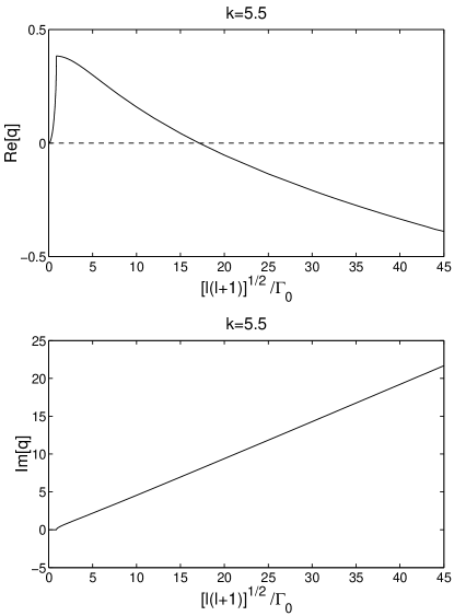
FIG. 2.: Perturbation growth rate, $q$, as a function of $\sqrt{l(l+1)}/\Gamma_{0}$. The upper and lower panels show ${\rm Re}[q]$ and ${\rm Im}[q]$ respectively.

The actual evolution of a perturbation is shaped by the fact that $\Gamma_{0}$ increases with time as $\Gamma_{0}^{2}\propto t^{-m_{1}}$. If initially the wavenumber of the perturbation is sufficiently large so that it is in the regime of large $l/\Gamma_{0}$, the perturbation will start to decay while oscillating. As time progresses, $l/\Gamma_{0}$ decreases and so both $\mid{\rm Re}[q]\mid$ and ${\rm Im}[q]$ decrease, the perturbation decays with slower speed and oscillates on longer timescales. As soon as the perturbation enters the regime of intermediate $l/\Gamma_{0}$, it starts to grow slowly over time and oscillate on even longer timescales. The growth rate slowly increases over time, but is always limited by the rather small upper bound, ${\rm Re}[q]\lesssim 0.38$. Eventually, the perturbation enters the regime of small $l/\Gamma_{0}$ and grows slowly without oscillating. As $t$ increases, the growth rate approaches zero, and so the perturbation saturates. Therefore, perturbations with large wavenumbers (short wavelengthes) grow when $1\lesssim l/\Gamma_{0}\lesssim 10$ only by a modest factor. In the case of intermediate wavenumbers, the perturbation goes through the two regimes of intermediate and small $l/\Gamma_{0}$. Therefore it grows slowly with some initial oscillations, but soon afterwards it stops oscillating and saturates. Perturbations with small wavenumbers stay in the regime of small $l/\Gamma_{0}$. The perturbation grows slowly without oscillating at the beginning but soon saturates.

The above results remain qualitatively the same for all values of $k>4.134$.

V Numerical Simulations

We have verified the above behavior by a direct integration of the partial different equations which determine the evolution of the perturbation variables, without assuming separability of the solutions with respect to $\xi$ and $t$. Instead of equations (122) – (125), we redefined the perturbation variables as

$$\delta\gamma^{2}(r,\theta,\phi,t)=\frac{1}{2}\Gamma_{0}^{2}\delta g(\xi,t)Y_{lm}(\theta,\phi),$$ (169)

$$\delta{\bf v}_{T}(r,\theta,\phi,t)=-\frac{1}{\Gamma_{0}^{2}}\delta v_{T}(\xi,t)\tilde{{\bf\nabla}}_{T}Y_{lm}(\theta,\phi),$$ (170)

$$\delta p(r,\theta,\phi,t)=\frac{2}{3}\rho_{1}\Gamma_{0}^{2}\delta f(\xi,t)Y_{lm}(\theta,\phi),$$ (171)

$$\delta n^{\prime}(r,\theta,\phi,t)=2n_{1}\Gamma_{0}^{2}\delta h(\xi,t)Y_{lm}(\theta,\phi).$$ (172)

Equations (128) – (139) were then replaced by four partial differential equations (PDEs) for the perturbation variables $\delta f(\xi,t)$, $\delta g(\xi,t)$ $\delta h(\xi,t)$ and $\delta v_{T}(\xi,t)$. We then solved for the evolution of these perturbation variables by numerically integrating the PDEs with appropriate initial values. In our numerical simulations, the outer boundary ($\xi=0$) is the shock front where the shock jump conditions are assumed to be satisfied. We can still define $\delta R$ as in equation (163). Then at the outer boundary the perturbation variables satisfy

$$\delta f(0,t)=\frac{df}{d\xi}X(t)+2(m_{1}+1)X(t)+2t\frac{dX(t)}{dt},$$ (173)

$$\delta h(0,t)=\frac{dh}{d\xi}X(t)+2(m_{1}+1)X(t)+2t\frac{dX(t)}{dt},$$ (174)

$$\delta g(0,t)=\frac{dg}{d\xi}X(t)+2(m_{1}+1)X(t)+2t\frac{dX(t)}{dt},$$ (175)

$$\delta v_{T}(0,t)=X(t).$$ (176)

The inner boundary is chosen to be sufficiently large so as to cover the entire similarity region which is bounded by a inner $C_{+}$ characteristic. This way, the values of the perturbation variables at the inner boundary can not affect the shock front.

The numerical simulations gave us the same behavior for the perturbations as the previously mentioned analytical results for the growth rate $q$. In Figure 3, we show the evolution of $X(t)$ in a numerical simulation with $k=5.5$ and $\l/\Gamma_{0}=75$. We plot $X(t)$ in the range $t\in[1,10]$ in the top panel and $t\in[1,100]$ in the bottom panel. Note that $X(t)$ describes the relative displacement of the perturbed shock radius from the unperturbed value and we set its initial value to be $X(t=1)=1.0$. From Figure 3 we see that $X$ oscillates over time over increasingly longer timescales and stops oscillating at late times. Its amplitude first decreases, then slowly increases and finally saturates. Overall it grows by a factor of $\sim 10$. These results are consistent with the previous discussion on the three regimes for the evolution of the perturbations.

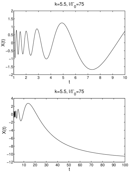
FIG. 3.: Evolution of $X(t)$ for $k=5.5$ and $\l/\Gamma_{0}=75$. The upper and lower panels show $t\in[1,10]$ and $t\in[1,100]$ respectively.

VI Conclusions

We have derived the self-similar solutions for an ultra-relativistic blast wave in an external medium with a density profile $\rho_{1}\propto r^{-k}$ and $k>4$. The solutions exist for $k$ larger than a critical value $k_{c}=4.134$. They describe the flow in the self-similar region bounded by the shock front and a $C_{+}$ characteristic. The shock front accelerates with Lorentz factor $\Gamma^{2}\propto t^{-m_{1}}$ and $m_{1}<-1.134$, while the $C_{+}$ characteristic accelerates with Lorentz factor $\gamma^{2}\propto t^{2}$. The energy and mass contained inside the self-similar region approach constant values as time diverges.

We have found that at large wavenumbers the perturbations first decay, then grow slowly over time and eventually saturate. The initial decay and the intermediate growth are accompanied by temporal oscillations. These small wavelength perturbations grow when $1\lesssim l/\Gamma_{0}\lesssim 10$ with an overall factor of $\sim 10$. At intermediate wavenumbers, the perturbations first grow slowly and then saturate. The initial growth is also accompanied by temporal oscillations. At small wavenumbers the perturbations grow monotonically in time but soon saturate. Our results also apply to expanding relativistic jets as long as the opening angle of the jet is larger than the inverse of its Lorentz factor.

In the collapsar model of gamma-ray bursts, a collimated relativistic outflow is generated due to the collapse of the core of a massive star. The outflow approaches the stellar envelope at a modest semi-relativistic speed but is expected to accelerate significantly across the sharp density gradient at the surface of the star[10]. Our results indicate that in the breakout phase perturbations are close to being stable in spherical symmetry. It is still possible, however, that the lateral expansion of the jet at breakout would be accompanied by instabilities. These instabilities may produce variations in the Lorentz factor of the jet needed in the internal shock model. They may also be responsible for the complex light curves observed in most GRBs. Current numerical simulations[10] lack adequate resolution at the stellar surface to follow the shock breakout and confirm the instabilities. We leave a detailed study of the instabilities associated with the lateral expansion of the jet for future work.

Acknowledgments.

This work was supported in part by grants from the Israel-US BSF (BSF-9800343) and NSF (AST-0071019, AST-0204514).

REFERENCES

[1]
R. D. Blandford & C. F. McKee, Phys. Fluids. 19, 1130 (1976).
[2]
P. Best & R. Sari, Phys. Fluids. 12, 3029 (2000).
[3]
R. Perna & M. Vietri, Astroph. J. Lett. 569, L47 (2002).
[4]
L. I. Sedov, Prikl. Mat. Mekh. 10, 241 (1946).
[5]
J. von Neumann, Blast Waves, Los Alamos Sci. Lab. Tech. Series
(Los Alamos, NM, 1947), Vol. 7.
[6]
G. I. Taylor, Proc. R. Soc. London Ser. A 201, 159 (1950).
[7]
E. Waxman & D. Shvarts, Phys. Fluids. A 5, 1035 (1993).
[8]
R. Sari, E. Waxman & D. Shvarts, Astroph. J. Suppl. Series.
127, 475 (2000).
[9]
J. P. Cox, Theory of Stellar Pulsation (Princeton: Princeton
Univ. Press) (1980).
[10]
W. Zhang, S. E. Woosley & A. I. MacFadyen,
Astroph. J., submitted, 2002, preprint astro-ph/0207436; and
references therein