Normal parameters for an analytic description of the CMB cosmological parameter likelihood

Abstract

The normal parameters are a non–linear transformation of the cosmological parameters whose likelihood function is very well–approximated by a normal distribution. This transformation serves as an extreme form of data compression allowing for practically instantaneous calculation of the likelihood of any given model, as long as the model is in the parameter space originally considered. The compression makes all the information about cosmological parameter constraints from a given set of experiments available in a useable manner. Here we explicitly define the normal parameters that work for the current CMB data, and give their mean and covariance matrix which best fit the likelihood function calculated by the Monte Carlo Markov Chain method. Along with standard parameter estimation results, we propose that future CMB parameter analyses define normal parameters and quote their mean and covariance matrix.

1 Introduction

The challenge of turning a CMB dataset into cosmological parameter constraints is one that has been solved by a series of data compressions. The information in the time–ordered data is compressed into a map (Wright et al., 1996; Tegmark, 1997a). The information in the map is then compressed into a power spectrum (Tegmark, 1997b; Bond et al., 1998, 2000; Wandelt et al., 2001; Bartlett et al., 2000; Hivon et al., 2002). Finally, the information in the power spectrum is then compressed into cosmological parameters (Lineweaver et al., 1997; Benoit, 2002).

This last step, however, is more of a data “explosion” than a data compression. Although the number of parameters is indeed small ($\sim 10$) the non–Gaussian distribution of their errors may be characterized by $10^{10}$ numbers for grid–based likelihood evaluation (Tegmark & Zaldarriaga, 2000) or perhaps as little as $30,000$ for the Monte-Carlo Markov Chain method (Christensen et al., 2001).

This explosion has undesirable consequences. The full constraining power of the data is not used by the cosmological community. Typically authors report not the full (cumbersome) likelihood, but projections or marginalizations of it down to one or at most two–dimensional spaces. Given the near–degeneracies that exist in the probability distribution, and its non-Gaussian nature, these final steps lose significant information.

Our work here provides the final step of compression in the data analysis pipeline. We compress the probability distribution of the cosmological parameters down to the $\sim 50$ parameters of an analytic form for the likelihood (a mean and covariance matrix). This step makes the full information in the parameter likelihood function easily useable.

Our procedure is analogous to the ‘radical compression’(Bond et al., 2000) used for compressing the uncertainty in the power spectrum estimates, whose distribtuion is also non–Gaussian. In both cases a non–linear variable transformation is used, with the property that the transformed variables are well–approximated by a normal distribution.

We were inspired to search for a set of normal parameters by a proposal that the $C_{l}$ can have a linear dependence on a set of well-chosen parameters that span the space of possible models (Kosowsky et al., 2002). Clearly such a parameter set would be tremendously valuable for parameter estimation since the $C_{l}$ for any given model could be calculated practically instantaneously simply by summing the terms in the first order Taylor expansion. Such a set would also, given sufficiently Gaussian errors on $C_{l}$, have errors with a normal distribution.

Although inspired by Kosowsky et al. (2002), our goal here is entirely different. It is to find a set of parameters (the normal parameters) for which the likelihood is Gaussian. Although the approximate linearity demonstrated by Kosowsky et al. (2002) gave us confidence to try to find a set of normal parameters, it by no means guaranteed success. The linear-response approximation has not yet been demonstrated to be sufficiently accurate for purposes of parameter estimation given MAP data (and certainly not given current data) and the errors on $C_{l}$ are not actually Gaussian.

While Kosowsky et al. (2002) are developing a tool for parameter estimation from CMB data, our work is aimed at being able to easily take full advantage of such parameter estimation. The most straightforward application of CMB data compressed in this form is for simultaneous analysis of CMB constraints with those from other cosmological probes. In the past to do this analysis one would have to entirely reproduce the reduction from bandpowers (plus their window functions, offset log–normal parameters, Fisher matrices, and calibration uncertainties) to cosmological parameter likelihoods. This procedure requires the organization of a lot of data as well as hundreds of thousands of angular power spectrum calculations. In contrast, with the compression to normal parameters in hand one need only perform a variable transformation and evaluate a $~{}10$–dimensional Gaussian. We use a similar set of parameters as KMJ, and demonstrate explicitly the validity of the normal approximation by numerical computation of the likelihood given current CMB data.

One can also simplify a probability distribution by choosing linear combinations of the parameters that diagonalize the covariance matrix, the so–called parameter eigenmodes (Efstathiou & Bond, 1999). However, the resulting parameters are still dependent and non–Gaussion if the distribution of the original parameters is non-Gaussian. We do find diagonalization of the covariance matrix of the normal parameters to be useful, both for our fitting procedure and for gaining an understanding of the nature of the constraints the data places on the parameter space.

We test our procedure on current data and provide the mean and covariance matrix to the normal parameters that best fit the likelihood given current data. As we go to press, this fit is now out of date due to the data from the Wilkinson Microwave Anisotropy Probe (WMAP) . However, we expect these data to further improve the validity of the normal approximation to the likelihood and thus our method will be of lasting value.

In section II we describe the normal parameters. In section III we describe our calculation of the exact likelihood via the Monte Carlo Markov Chain method (Christensen et al., 2001). In section IV we describe our procedure for finding the mean and covariance matrix that provide the best fit to our MCMC–calculated likelihood. In section V we present our results. In section VI we discuss applications and conclude.

2 The normal parameters

The normal parameters are a non-linear combination of the six cosmological parameters that we consider here – $\omega_{b}$, $\omega_{d}$, $\Omega_{\Lambda}$, $z$, $A\equiv(2.73\times 10^{6})^{2}\,{\rm Mpc}^{-3}P_{\Phi}(0.05\,{\rm Mpc}^{-1})$ and $n_{s}$ (baryon density, dark matter density, dark energy density, reionization redshift, amplitude and scalar tilt of primordial power spectrum respectively). In particular, we replace $\Omega_{\Lambda}$, $A$ and $n_{s}$ by

$$\Theta_{s} \simeq \Theta_{s}^{E}\equiv r_{s}/d_{A}$$ (1)

$$A^{*} \equiv {A\over 76,000}\,\left({0.05\,{\rm Mpc}^{-1}\over k_{\rm pivot}}\right)^{1-n_{s}}e^{-2\tau}$$ (2)

$$t \equiv \frac{1}{\sqrt{w_{b}}}\,2^{n_{s}-1}$$ (3)

where $r_{s}$ is the sound horizon at recombination, $d_{A}$ is the angular diameter distance to the recombination surface and we take $k_{\rm pivot}=0.067\,{\rm Mpc}^{-1}$. The distinction between $\Theta_{s}$ and $\Theta_{s}^{E}$ is explained below. The numerical factors are chosen so that $A^{*}$ is of order unity. We use $\tau$ to denote the optical depth to Thomson scattering from here back to some time before reionization and after recombination. The resulting variable set, $\{\omega_{b},\omega_{d},\Theta_{s},A^{*},t,z\}$, has a probability distribution, given CMB data, that is well–approximated by a Gaussian as we will demonstrate below.

We chose the normal parameters by considering what combinations of cosmological parameters affect the features in the angular power spectrum over the range in which the data are highly constraining ($100\lesssim l\lesssim 500$). The parameter $A^{*}$ describes the overall amplitude, $t$ is chosen to correlate with the ratio of the amplitude of the second peak to the first peak (at fixed $\omega_{m}$), and $\Theta_{s}$ scales the features horizontally.

Hu et al. (2001) have investigated this phenomenology as well. For $\Theta_{S}$ we use their approximation to the angular size of the sound horizon, which has the advantage of being an algebraic expression, rather than the exact sound horizon, $\Theta_{s}^{E}$. This distinction is important because they can differ by more than the uncertainty in $\Theta_{S}$. Hu et al. (2001) also define a parameter $H_{2}$ analogous to our $t$ but with a different parameter dependence.

The importance of $\Theta_{s}$ for understanding the $C_{l}$ is widely recognized (Efstathiou & Bond, 1999; Tegmark & Zaldarriaga, 2000; Hu et al., 2001; Kaplinghat et al., 2002; Kosowsky et al., 2002). It is one of the best–determined cosmological quantities: $\Theta_{s}=0.^{\circ}59\pm 0.^{\circ}01$ (Knox et al., 2001).

The parameter $A^{*}$ sets the overall amplitude of the spectrum at $l\gtrsim 100$. At these $\ell$ values, Thomson scattering depresses the amplitude by $\exp(-2\tau)$. The value of $k_{\rm pivot}$ was chosen to decorrelate $A^{*}$ and $n_{S}$. In an idealized case with uniform relative error bars on $l(l+1)C_{l}/(2\pi)$ from some $l_{\rm min}$ to $l_{\rm max}$ we would expect $k_{\rm pivot}=\sqrt{l_{\rm min}l_{\rm max}}/\eta_{0}$ where $\eta_{0}=(14\pm 0.6)$ Gpc is approximately the coordinate distance to the last–scattering surface. Taking $l_{\rm min}=10$ and $l_{\rm max}=1000$ we expect $k_{\rm pivot}\sim 0.007\,{\rm Mpc}^{-1}$. At fixed $\tau$ (or $z$) we find this value works well. Allowing $\tau$ to vary leads to a correlation with $n_{S}$. A result of this correlation is that decorrelation between $A^{*}$ and $n_{S}$ is best done with a much larger $k_{\rm pivot}$ of about $0.067\,{\rm Mpc}^{-1}$. The $\tau$-$n_{S}$ correlation arises because both rely considerably on $C_{l}$ measurements at $l<100$.

The least “normal” of the normal parameters is $z$, which is not very well–constrained by CMB data. The situation may improve quite soon with large–angle polarization data from MAP (Kaplinghat et al., 2002). Or, it is already not a problem if one interprets observation of a Gunn–Peterson trough in a $z=6.3$ quasar as indicating $z_{\rm RI}\simeq 6.3$ (Becker et al., 2001; Fan et al., 2002). We caution that though the data indicate the amount of neutral Hydrogen in the inter–galactic medium is rising from zero, how much the fraction of free electrons is increasing with $z$ is highly unconstrained (Kaplinghat et al., 2002).

We assume a step function transition of the ionization fraction from 0 to 1 at redshift $z$. For the flat models we consider this results in an optical depth of

$$\tau=0.038\omega_{b}h/\omega_{m}\left[\sqrt{\Omega_{\Lambda}+\Omega_{m}(1+z)^{3}}-1\right]$$ (4)

(Hu & White, 1997; Kaplinghat et al., 2002). We settled on $z$ as a normal parameter after trial and error. We have found $z$ to be more normal than either $\tau$ or $\exp{-2\tau}$.

We have not included tensor perturbations, curvature or dark energy models with $w\equiv p/\rho\neq-1$ in our analysis and so our results strictly only apply with these assumptions. Including all these variations (at fixed $\Theta_{s}$) would only alter the $C_{l}$ at $l\lesssim 60$. Their inclusion would therefore affect our constraints on $z$ and $n_{S}$ (and therefore $t$), but not $A^{*}$, $\Theta_{s}$, $\omega_{b}$ or $\omega_{d}$.

3 Likelihood Calculation

What we want to know is, given the data and any other assumptions we make about the world, what is the probability distribution of the parameters? This posterior probability distribution can be calculated by use of Bayes’ theorem which states:

$$P({\vec{\theta}}|d)\propto P(d|{\vec{\theta}})P_{\rm prior}({\vec{\theta}})\,.$$ (5)

where $d$ refers to data and the proportionality constant is chosen to ensure $\int P({\vec{\theta}}|d)d{\vec{\theta}}=1$. With a uniform prior this simply reduces to $P({\vec{\theta}}|d)\propto P(d|{\vec{\theta}})$. This probability of the data given the parameters is, when thought of as a function of the parameters, called the likelihood, ${\cal L}({\vec{\theta}})$.

Often we are interested in the posterior probability distribution for one or two parameters alone. This marginalized posterior is given by integrating over the other parameters. For example:

$$P(\theta_{1},\theta_{2}|d)=\int\Pi_{i=3}^{n}d\theta_{i}{\cal L}(\vec{\theta})P_{\rm prior}(\vec{\theta})$$ (6)

where $n$ is the number of parameters. We use the prior to incorporate non–CMB information such as that the redshift of reionization must be greater than 6.3 (Becker et al., 2001).

In the following subsections we discuss first how we evaluate the likelihood function at a single point and then how we evaluate it over a large parameter space and produce marginalized posterior distributions.

3.1 Likelihood evaluation

Here we take the data to be the measured averages of the angular power spectrum (called bandpowers), $D_{i}^{d}$. The expected signal contribution to $D_{i}^{d}$ is given by an average over the power spectrum:

$$D^{s}_{i}=\sum_{l}u^{2}_{\alpha(i)}f_{il}{\cal C}_{l}(\vec{\theta})$$ (7)

where $u_{\alpha(i)}$ is the calibration parameter for dataset $\alpha$ and ${\cal C}_{l}\equiv l(l+1)C_{l}/(2\pi)$ is the angular power spectrum.

The uncertainty in the $D_{i}$ is non–Gaussian but well–approximated by the offset log–normal form of Bond et al. (2000). Specifically, ${\cal L}=\exp(-\chi^{2}/2)$ where

$$\chi^{2} = \sum_{i,j}\left(Z_{i}^{\rm s}-Z_{i}^{\rm d}\right)M_{ij}^{Z}\left(Z_{j}^{\rm s}-Z_{j}^{\rm d}\right)+\chi^{2}_{\rm expt};$$ (8)

$$\chi^{2}_{\rm expt} \equiv \sum_{\alpha}{(u_{\alpha}-1)^{2}\over\sigma_{\alpha}^{2}}+(b-\bar{b})^{2}/\sigma_{b}^{2};$$ (9)

$$Z_{i}^{\rm d} \equiv \ln(D_{i}^{d}+x_{i});$$ (10)

$$Z_{i}^{\rm s} \equiv \ln\left(D_{i}^{s}+x_{i}\right);$$ (11)

$$M_{ij}^{Z} \equiv M_{ij}\left(D_{i}^{d}+x_{i}\right)\left(D_{j}^{d}+x_{j}\right)\quad\mbox{no sum};$$ (12)

where $M_{ij}$ is the weight matrix for the band power data $D_{i}^{d}$. The expt label is for experimental parameters. These include the calibration parameters and a beam–width parameter, $b$, for the one experiment with significant and quantified uncertainty in their beam width. For simplicity, we take the prior probability distribution for the experimental parameters to be normally distributed. Since the datasets have already been calibrated, the mean of the calibration parameters is at $\bar{u}_{\alpha}=1$. The calibration parameter index, $\alpha$, is a function of $i$ since different power spectrum constraints from the same dataset all share the same calibration uncertainty.

We include bandpower data from Boomerang, the Degree Angular Scale Interferometer (DASI; Halverson et al., 2002), Maxima (Lee et al., 2001)), the COsmic Background Explorer(COBE; Bennett et al., 1996), VSA and CBI. The weight matrices, band powers and window functions are publicly available for both VSA and DASI. For COBE we approximate the window functions as tophat bands; all other information is available in Bond et al. (2000) and in electronic form with the DASh package. For Boomerang, CBI and Maxima we approximate the window functions as top-hat bands, the weight matrices as diagonal and the log-normal offsets, $x$, as zero. The Boomerang team report the uncertainty in their beam full-width at half-maximum (fwhm) as $12.9\pm 1.4$ minutes of arc. We follow them in modelling the departure from the nominal (non-Gaussian) beam shape as a Gaussian. For the Boomerang $D_{i}^{s}$, we replace ${\cal C}_{l}$ in Eq. 7 with ${\cal C}_{l}\exp(-l^{2}b^{2})$. We do not allow the fwhm to go below 11’.5 or above 14’.3; i.e. we give such fluctuations zero probability. To reduce our sensitivity to beam errors, for Boomerang and Maxima we only use bands with maximum $l$-values less than 1000. For CBI we use their broader mosaic’ed fields with bandpowers that extend to $l=1900$.

3.2 Exploring the Parameter Space

Our first step in exploring the high–dimensional parameter space is the creation of an array of parameter values called a chain, where each element of the array, $\vec{\theta}$, is a location in the $n$-dimensional parameter space. The chain has the useful property once it has converged that $P(\vec{\theta}\in R)=N(\vec{\theta}\in R)/N$ where the left–hand side is the posterior probability that $\vec{\theta}$ is in the region $R$, $N$ is the total number of chain elements and $N(\vec{\theta}\in R)$ is the number of chain elements with $\vec{\theta}$ in the region $R$. Once the chain is generated one can then rapidly explore one–dimensional or two–dimensional marginalizations in either the original parameters, or in derived parameters, such as $t_{0}$. Calculating the marginalized posterior distributions is simply a matter of histogramming the chain.

The chain we generate is a Monte Carlo Markov Chain (MCMC) produced via the Metropolis–Hastings algorithm described in Christensen et al. (2001). The candidate–generating function for an initial run was a normal distribution for each parameter. Subsequent runs used a multivariate–normal distribution with cross–correlations between cosmological parameters equal to those of the posterior as calculated from the initial run.

The covariance matrix of the candidate–generating function, $C_{G}$ is actually a scaled version of the posterior covariance matrix, $C_{P}$: $C_{G}=aC_{P}$. Proper choice of $a$ is important if the movement through parameter space is to be efficient. If $a$ is too low, the acceptance rate will be high, but the typical step size will be small and a full sampling of the parameter space will take a long time. If $a$ is too high then most steps will be to regions of greatly reduced probability, the acceptance rate will therefore be low and once again a full sampling of the parameter space will take a long time. As a useful measure of the speed at which we sample the parameter space, we define the step distance to be:

$$\Delta\sigma_{n,n-1}=\sqrt{\sum_{i}\Delta\theta_{i}C_{P,ij}^{-1}\Delta\theta_{j}};$$ (13)

where $\Delta\theta_{i}$=$(\theta_{n})_{i}-(\theta_{n-1})_{i}$, $n$ is the iteration number and $i$ enumerates the parameters. In other words we are using the inverse covariance matrix as the distance metric for the parameter space. We automatically adjust $a$ in the first 20,000 samples of a run to maximize this average step distance. We find it has a fairly broad plateau between 0.3 and 0.7. In practice we calculate the square of the distance with the slightly simpler expression: $\sum_{i}(\Delta\theta_{i})^{2}/C_{P,ii}$.

All of our results are based on an MCMC run consisting of 754,000 iterations. For the “burn-in” the initial 20,000 samples were discarded, and the remaining set was thinned by accepting every 25th iteration, resulting in nearly 30,000 samples. The acceptance rate was 43% with $a=.37$ and an average step distance of 0.25 indicating highly efficient movement through the parameter space. We used the CODA software (Best et al., 1995) to confirm that the chain passed the Referty-Lewis convergence diagnostics and the Heidelberger-Welch stationarity test.

4 Fitting to the Likelihood

We do not fit directly to the ten–dimensional likelihood or even to its marginalization down to the six cosmological parameters. The reason is that in the high–dimensional spaces, the likelihood is very sparsely sampled. For a fairly coarse grid with 8 steps in each direction, there would be $6^{8}>250,000$ grid points and yet we have only 30,000 samples. Only with the marginalizations down to even lower–dimensions does the likelihood become densely sampled.

Instead we fit to the two–dimensional marginalized likelihoods and from these fits reconstruct the full result. We typically use 50 bins in each parameter which results in about 100 samples in the most-likely of the 2500 bins.

We do this fitting in the normal parameter space. That is, at each point in the chain we calculate the value of the two normal parameters of interest and histogram that point accordingly. For every such pair of normal parameters we find $\bar{\theta}_{i}$ and $F^{2d}_{ij}$ that give the best–fit two–dimensional Gaussian likelihood where

$${\cal L}_{2d}^{N}\propto\exp\left[-{1\over 2}\left(\theta_{i}-\bar{\theta}_{i}\right)F^{2d}_{ij}\left(\theta_{j}-\bar{\theta}_{j}\right)\right].$$ (14)

From these $n\times(n-1)/2$ ($=15$ for $n=6$) fits we reconstruct the six–dimensional Gaussian. We exploit a property of Gaussian distributions that the inverse of $F^{2d}_{ij}$ gives the elements of the covariance matrix in the full higher–dimensional space: $C_{ij}=(F^{2d})^{-1}_{ij}$. Thus we uniquely determine the 15 independent off-diagonal elements of the 6 by 6 covariance matrix. The diagonal elements are over–determined with five estimates of $C_{ii}$ for each $i$; we average these together for the final estimate. The full covariance matrix is then inverted, giving the 6–dimensional Fisher-matrix of the likelihood function. The $\bar{\theta}_{i}$ are also averaged to produce an estimate of the likelihood maximum.

Note that each of the off-diagonal elements is obtained from a 2D gaussian fit to different variable pairs. Therefore there is no guarantee that the covariance matrix built from these 2x2 blocks will necessarily be positive-definite (which a true covariance matrix should be). We employ an iterative procedure to solve the above problem. We first increase the diagonal terms of $C$ until $C$ is positive-definite. We then invert $C$ to get the Fisher matrix $F=C^{-1}$ and find its eigenmodes. Now we identify these eigenmodes as the “new normal parameters” and perform the 2D fit procedure again (this step is not computationally intensive). The resulting covariance matrix (from the 2D fits) will be close to diagonal and hence positive definite. We repeat this procedure typically about 15 times by which time the changes in the covariance matrix are less than 3%. We have also verified that the final result is insensitive to the arbitrary adjustments to the covariance matrix (to make it positive-definite) in the first step.

The end result is an approximate likelihood, ${\cal L}^{N}$, with most likely values $\bar{\theta}_{i}$ and covariance matrix $C_{ij}$:

$$-2\ln{{\cal L}^{N}}=\left(\theta_{i}-\bar{\theta}_{i}\right)C^{-1}_{ij}\left(\theta_{j}-\bar{\theta}_{j}\right).$$ (15)

If we denote the cosmological parameters with $\vec{c}$ and the normal parameters with $\vec{\theta}$, the likelihood of the cosmological parameters is given by

$${\cal L}^{c}(\vec{c})={\cal L}^{N}(\vec{\theta}(\vec{c}))|{\partial\vec{c}\over\partial\vec{\theta}}|$$ (16)

where

$$|{\partial\vec{c}\over\partial\vec{\theta}}|={\partial\Theta_{s}\over\partial\Omega_{\Lambda}}{A^{*}\over A}\left({0.05\,{\rm Mpc}^{-1}\over k_{\rm pivot}}\right)^{n_{s}-1}b\ln 2$$ (17)

is the Jacobian of the variable transformation.

5 Results

In Table 1 we show the parameters of ${\cal L}^{N}$ that make it a good approximation to our MCMC–calculated likelihood. For ease of interpreting the magnitude of the off–diagonal elements we have shown the correlation matrix which is given by $C_{ij}/\sqrt{C_{ii}C_{jj}}$ instead of $C_{ij}$ itself.

We compare the fit to the exact likelihood in Fig. 1 which shows 6 of the 15 possible marginalizations down to two dimensions. The marginalization of the normal fit is done by a Monte Carlo process. We use the normal fit to rapidly generate a chain whose elements are samples from the normal distribution. We can then manipulate this chain (e.g., to marginalize down to 2 dimensions) just like we manipulate the Markov chains.

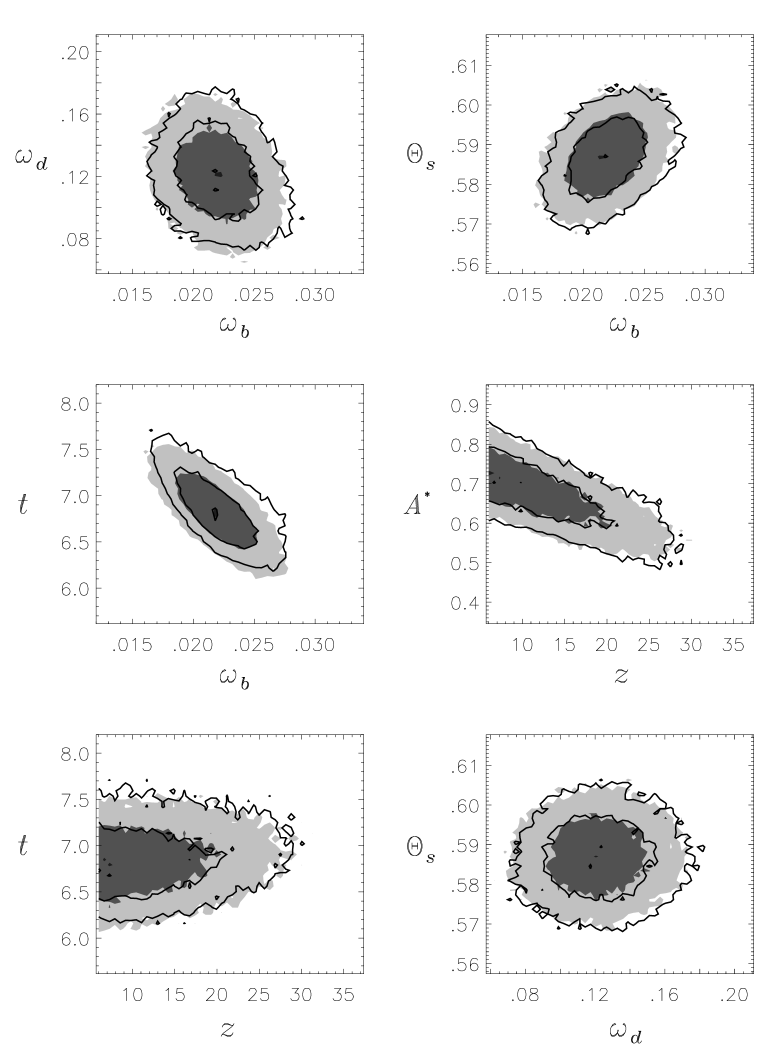
Figure 1: Comparison of the two–dimensional marginalized posterior probability distributions of the normal parameters for the normal fit (shading) and the MCMC–calculated likelihood (contours). Contours and shading show where the probability is above $\exp(-2.3/2)$ and $\exp(-6.17/2)$ of the maximum value.

All six marginalizations down to one dimension are shown in Fig. 2. One can see that the fit provides an excellent match to the exact one–dimensional likelihoods.

Note that although the fit is Gaussian in the six–dimensional space, the priors implicit in the marginalization down to one dimension result in slightly non–Gaussian one–dimensional likelihoods. This is because the marginalization is not done over the full parameter space but has the constraints $z>6$, $0<\Omega_{\Lambda}<0.9$, $0.45<h<0.95$ and $0.02<\Omega_{m}<1.1$.

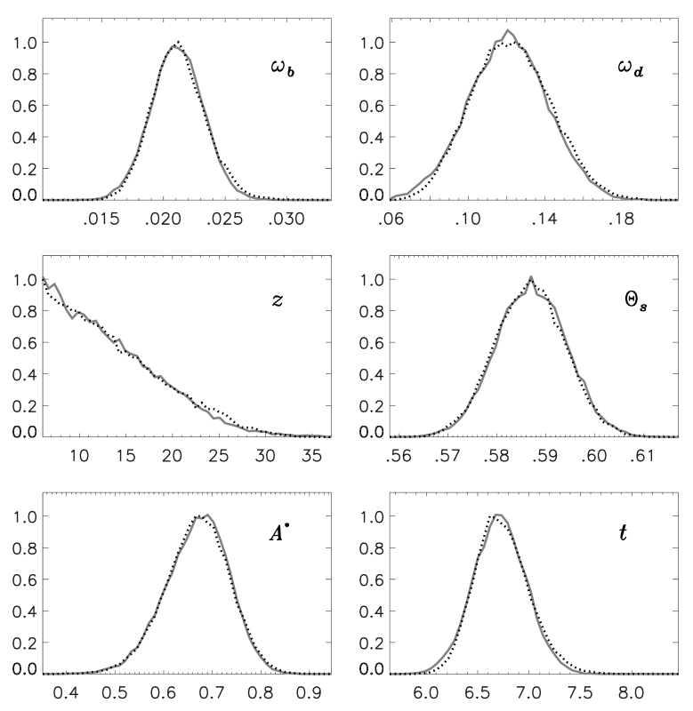
Figure 2: Comparison of the one–dimensional marginalized posterior probability distributions of the normal parameters for the normal fit (solid, red) and the MCMC–calculated likelihood (dotted, black).

Our normal fit to the likelihood can also be used to obtain marginalized constraints on the cosmological parameters. Marginalizations down to two dimensions and one dimension are shown in Figures 3 and 4 respectively. Note that the highly non–Gaussian distributions of the cosmological parameters are described well by the fit that is Gaussian in the normal parameters.

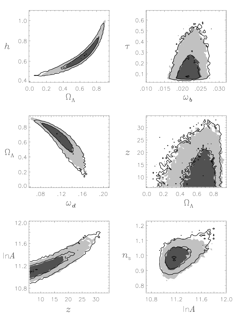
Figure 3: As in Fig. 1 but for other parameters.

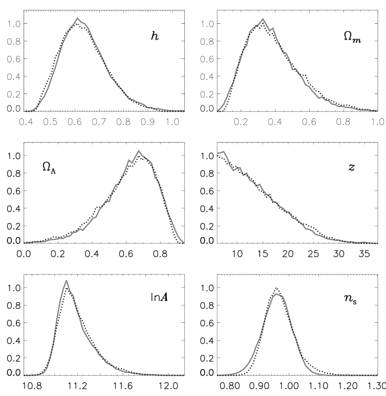
Figure 4: As in Fig. 2 but for other parameters.

The eigenmodes and eigenvalues $\lambda$ are shown in Table 2. These are the eigenmodes of the fractional Fisher matrix, $F^{f}_{ij}=\bar{\theta}_{i}F^{a}_{ij}\bar{\theta}_{j}$ where $\bar{\theta}_{i}$ are the best–fit values of the normal parameters. We look at the fractional Fisher matrix so its eigenvalues quantify the fractional error and not the absolute error. The eigenvectors are ordered from highest eigenvalue to lowest eigenvalue. We see that current CMB data constrain four parameters at the 10% level or better. As expected, the best–constrained eigenvector is predominantly $\Theta_{s}$ and the worst–constrained is almost entirely $z$. The second–from–worst is $\omega_{d}$, though even it is farily well–constrained with $\sqrt{\lambda}=0.16$. Eigenvectors 2, 3 and 4 are mostly $t$, $A^{*}$ and $\omega_{b}$ respectively, though each with significant amounts of other parameters mixed in.

We have also explored the likelihood distribution of the parameter set proposed by Kosowsky et al. (2002). In 2-D projections, most pairs of parameters do look Gaussian. An exception is any pair involving their variable ${\cal Z}\equiv\exp{(-2\tau)}$, which is significantly less Gaussian than the variable we have used to parameterize reionization: the redshift of reionization, $z$.

6 Discussion and Conclusions

We have defined a set of parameters that, given current data, have a likelihood that is normally distributed. Of course, our simple fit to the likelihood surface will very soon be out-of-date due to the expected MAP data. Still, we expect the technique to continue to be useful. Generally, as data become more constraining, the Gaussian approximation becomes better.

The challenge in the future will be to provide good parameterizations for those parameters that remain poorly determined. Some of these only have their effects at low $\ell$, such as the parameters governing reionization. For these it may be useful to define parameters for which $\ln{C_{l}}$ is linear, since the errors in this quantity are very nearly normally distributed at low $\ell$ Bond et al. (2000). Other physical effects, such as gravitational lensing, are only important at high $\ell$ where, if instrument noise is the dominant contribution to error in $C_{l}$, then $C_{l}$ will be nearly normally distributed. For these one would want to use parameterizations for which $C_{l}$ is linear.

An analytic form for the likelihood makes the actual application of CMB parameter constraints to cosmological questions much easier. One application is to quickly calculate constraints on various combinations of the cosmological parameters such as $\sigma_{8}$ (Holder, 2002) or the age, $t_{0}$ (Knox et al., 2001). Another is to combine the CMB results with those from other probes to improve constraints or search for inconsistencies (Wang et al., 2002). Or one can forecast expected constraints from a combination of the CMB and other probes such as supernovae (Frieman et al., 2002) or galaxy cluster number counts (Levine et al., 2002). Although these applications are possible without an analytic form for the CMB likelihood, such a form greatly simplifies the analysis.

Use of normal parameters will also improve the efficiency of Monte Carlo evaluations of the likelihood, by providing an analytic generating function that is well–matched to the actual likelihood. Although the statistical properties of the post–convergence chain do not depend on the generating function used, the time required for convergence depends critically on the generating function. In particular the chain rapidly converges if the generating function approximates the likelihood well. Clearly, this issue becomes more important for larger parameter spaces. A practical way to implement the use of normal parameters in generating Monte Carlo Markov chains would be to create a small chain, derive the normal parameters and the gaussian approximation to the likelihood, and then use this gaussian likelihood as the generating function.

In this paper we have explicitly given an analytic form for the likelihood (given a certain data set) of cosmological parameters and shown it to be an excellent approximation to the MCMC–calculated likelihood. We view this as the final step in a long data-reduction chain that begins with the time–ordered data.

	$\omega_{b}$	$\omega_{d}$	$z$	$\Theta_{s}$	$A^{*}$	$t$
$\omega_{b}$	1.000	-0.2270	-0.6840	0.3792	0.2572	0.05676
$\omega_{d}$	-0.2270	1.000	-0.03926	0.008238	-0.1875	0.2819
$z$	-0.6840	-0.03926	1.000	-0.2831	0.2031	-0.1503
$\Theta_{s}$	0.3792	0.008238	-0.2831	1.000	0.003574	0.2755
$A^{*}$	0.2572	-0.1875	0.2031	0.003574	1.000	-0.8229
$t$	0.05675	0.2819	-0.1503	-0.8229	0.2755	1.000
$\sqrt{C_{ii}}$	$0.0022$	0.023	0.26	0.0073	11.5	0.088
mean	0.021	0.125	6.719	0.587	3.75	0.69

Table 1: Correlation matrix, rms and mean of the normal fit to the likelihood.

eigenvector	$\omega_{b}$	$\omega_{d}$	$z$	$\Theta_{s}$	$A^{*}$	$t$	$\lambda^{-1/2}$
1	0.02327	0.01554	-0.004625	0.9852	-0.1152	0.1240	0.0090
2	0.3664	0.08785	-0.01180	-0.1448	-0.1890	0.8951	0.015
3	-0.2624	-0.1551	0.03314	0.07245	0.8923	0.3232	0.048
4	0.8759	0.1070	0.007523	0.05664	0.3731	-0.2811	0.10
5	-0.1706	0.9779	0.01899	0.002654	0.1190	-0.0003358	0.16
6	0.009783	-0.01314	0.9992	$-2.9\times 10^{-5}$	-0.03743	0.002542	2.8

Table 2: Normal parameter Eigenvectors and the errors on their amplitudes, $\lambda^{-1/2}$.

References

- Bartlett et al. (2000) Bartlett, J. G., Douspis, M., Blanchard, A., & Le Dour, M. 2000, A&AS, 146, 507
- Becker et al. (2001) Becker, R. H., Fan, X., White, R. L., Strauss, M. A., Narayanan, V. K., Lupton, R. H., Gunn, J. E., Annis, J., Bahcall, N. A., Brinkmann, J., Connolly, A. J., Csabai, I. ., Czarapata, P. C., Doi, M., Heckman, T. M., Hennessy, G. S., Ivezić, Ž., Knapp, G. R., Lamb, D. Q., McKay, T. A., Munn, J. A., Nash, T., Nichol, R., Pier, J. R., Richards, G. T., Schneider, D. P., Stoughton, C., Szalay, A. S., Thakar, A. R., & York, D. G. 2001, AJ, 122, 2850
- Bennett et al. (1996) Bennett, C. L., Banday, A. J., Gorski, K. M., Hinshaw, G., Jackson, P., Keegstra, P., Kogut, A., Smoot, G. F., Wilkinson, D. T., & Wright, E. L. 1996, ApJ, 464, L1
- Benoit (2002) Benoit, A. e. a. 2002, astro-ph/0210306
- Best et al. (1995) Best, N. G., Cowles, M. K., & Vines, S. K. 1995, CODA: Convergence, Diagnosis, and Output Software for Gibbs Sampler Output (version 0.30; Cambridge: MRC Biostatistics Unit)
- Bond et al. (1998) Bond, J. R., Jaffe, A. H., & Knox, L. 1998, Phys. Rev. D, 57, 2117
- Bond et al. (2000) —. 2000, ApJ, 533, 19
- Christensen et al. (2001) Christensen, N., Meyer, R., Knox, L., & Luey, B. 2001, Classical Quantum Gravity, 18, 2677
- Efstathiou & Bond (1999) Efstathiou, G. & Bond, J. R. 1999, MNRAS, 304, 75
- Fan et al. (2002) Fan, X., Narayanan, V. K., Strauss, M. A., White, R. L., Becker, R. H., Pentericci, L., & Rix, H. 2002, AJ, 123, 1247
- Frieman et al. (2002) Frieman, J. A., Huterer, D., Linder, E. V., & Turner, M. S. 2002, astro-ph/0208100
- Halverson et al. (2002) Halverson, N. W., Leitch, E. M., Pryke, C., Kovac, J., Carlstrom, J. E., Holzapfel, W. L., Dragovan, M., Cartwright, J. K., Mason, B. S., Padin, S., Pearson, T. J., Readhead, A. C. S., & Shepherd, M. C. 2002, ApJ, 568, 38
- Hivon et al. (2002) Hivon, E., Górski, K. M., Netterfield, C. B., Crill, B. P., Prunet, S., & Hansen, F. 2002, ApJ, 567, 2
- Holder (2002) Holder, G. 2002, astro-ph/0207600
- Hu et al. (2001) Hu, W., Fukugita, M., Zaldarriaga, M., & Tegmark, M. 2001, ApJ, 549, 669
- Hu & White (1997) Hu, W. & White, M. 1997, ApJ, 479, 568
- Kaplinghat et al. (2002) Kaplinghat, M., Knox, L., & Skordis, C. 2002, ApJ, 578, 665, astro-ph/0203413
- Kaplinghat et al. (2002) Kaplinghat, M. et al. 2002, astro-ph/0207591
- Knox et al. (2001) Knox, L., Christensen, N., & Skordis, C. 2001, ApJ, 563, L95
- Kosowsky et al. (2002) Kosowsky, A., Milosavljevic, M., & Jimenez, R. 2002, Phys. Rev. D, 66, 63007
- Lee et al. (2001) Lee, A. T., Ade, P., Balbi, A., Bock, J., Borrill, J., Boscaleri, A., de Bernardis, P., Ferreira, P. G., Hanany, S., Hristov, V. V., Jaffe, A. H., Mauskopf, P. D., Netterfield, C. B., Pascale, E., Rabii, B., Richards, P. L., Smoot, G. F., Stompor, R., Winant, C. D., & Wu, J. H. P. 2001, ApJ, 561, L1
- Levine et al. (2002) Levine, E. S., Schulz, A. E., & White, M. 2002, ApJ, 577, 569
- Lineweaver et al. (1997) Lineweaver, C. H., Barbosa, D., Blanchard, A., & Bartlett, J. G. 1997, A&A, 322, 365
- Tegmark (1997a) Tegmark, M. 1997a, ApJ, 480, L87+
- Tegmark (1997b) —. 1997b, Phys. Rev. D, 55, 5895
- Tegmark & Zaldarriaga (2000) Tegmark, M. & Zaldarriaga, M. 2000, ApJ, 544, 30
- Wandelt et al. (2001) Wandelt, B. D., Hivon, E., & Górski, K. M. 2001, Phys. Rev. D, 64, 83003
- Wang et al. (2002) Wang, X., Tegmark, M., & Zaldarriaga, M. 2002, Phys. Rev. D, 65, 123001
- Wright et al. (1996) Wright, E. L., Hinshaw, G., & Bennett, C. L. 1996, ApJ, 458, L53+