It is argued why, contrary to expectations, steep brane-inflation cannot really help in overcoming the $\eta$-problem of quintessential inflation model-building. In contrast it is shown that the problem is substantially ameliorated under the curvaton hypothesis. This is quantified by considering possible modular quintessential inflationary models in the context of both standard and brane cosmology.

1 Introduction

Recent high redshift SN-Ia observations suggest that the Universe at present is undergoing accelerated expansion [1]. These findings are consistent with the latest precise observations on the anisotropy of the Cosmic Microwave Background Radiation (CMBR) [2] and also with the observations of the Large Scale Structure (LSS) distribution of galactic clusters and superclusters [3]. Consequently, modern cosmology seems to have reached a point of concordance, which may be characterized by the following: We seem to live on a spatially flat, homogeneous and isotropic Universe which, at present, is comprised by about 1/3 of pressureless matter (dark matter mostly) and 2/3 by some other substance, with negative pressure, referred to as dark energy. The nature of this dark energy, however, remains elusive.

The above picture is in excellent agreement with the inflationary paradigm, which was initially introduced to solve the horizon and flatness problems of the Standard Hot Big Bang (SHBB) (and some other problems that were thought to be important at the time, such as the monopole problem) [4][5]. Inflation, in general, predicts a spatially flat Universe and also provides a superhorizon spectrum of curvature perturbations that result in adiabatic density perturbations which can successfully seed the formation of the observed LSS and the CMBR anisotropy. The spectrum of the curvature perturbations is predicted to be very near scale invariance, which agrees remarkably with the latest data. Hence, the inflationary paradigm is now considered by most cosmologists as the necessary extension of the SHBB, in order to form the Standard Model of Cosmology.

The successes of the inflationary paradigm have motivated many authors to consider a similar type of solution to the dark energy problem at present. Thus, it has been suggested that the current accelerated expansion of the Universe is due to a late-time inflationary period driven by the potential density of a scalar field $Q$, called quintessence (the fifth element, added to cold dark matter, hot dark matter (neutrinos), baryons and photons) [7]. The aim for introducing quintessence was to avoid resurrecting the embarrassing issue of the cosmological constant $\Lambda$, which, if called upon to account for the dark energy, would have to be fine-tuned to the incredible level of $\Lambda^{2}\sim 10^{-120}M_{P}^{4}$, where $M_{P}$ is the Planck mass, i.e. the natural scale for Einstein’s $\Lambda$.

However, it was soon realized that quintessence suffered from its own fine-tuning problems [9]. Indeed, in fairly general grounds it can be shown that at present $Q\sim M_{P}$ (if originally at zero) with a mass $m_{Q}\sim 10^{-33}$eV, which is very hard to understand in the context of supergravity theories, where we expect the flatness of the potential to be lifted on internal-space distances of the order of $M_{P}$. In addition, the introduction of yet again another unobserved scalar field (on top of the inflaton field which drives the early Universe inflationary period) seems unappealing. Finally, a rolling scalar field introduces another tuning problem, namely that of its initial conditions.

A compelling way to overcome the difficulties of the quintessence scenario is to link it with the rather successful inflationary paradigm. This is quite natural since both inflation and quintessence are based on the same idea; that the Universe undergoes accelerated expansion when dominated by the potential density of a scalar field, which rolls down its almost flat potential. This unified approach has been named quintessential inflation [10] and is attained by identifying $Q$ with the inflaton field $\phi$. In quintessential inflation the scalar potential of $\phi$ is such that it causes two phases of accelerated expansion, one at early and the other at late times.

However, the task of formulating such a potential is not easy and this is why not many successful attempts exist in the literature [10][11][12][13][14][15][16]. Indeed, successful quintessential inflation has to account not only for the requirements of both inflation and quintessence [17] but also for a number of additional considerations. In particular, the minimum of the potential (taken to be zero, otherwise there is no advantage over the cosmological constant alternative) must not have been reached yet by the rolling scalar field, in order for the residual potential density not to be zero at present. This requirement is typically satisfied by potentials, which have their minimum displaced at infinity, $V(\phi\rightarrow\infty)\rightarrow 0$, a feature referred to as “quintessential tail”. Thus, quintessential inflation is a non-oscillatory inflationary model [18]. Another requirement is that of a “sterile” inflaton, whose couplings to the Standard Model (SM) particles are strongly suppressed. This is necessary in order to ensure the survival of the inflaton until today, so that it can become quintessence. Thus, in quintessential inflation the inflaton field does not decay at the end of the inflationary period into a thermal bath of SM particles. Instead, the reheating of the Universe is achieved through gravitational particle production during inflation, a process refereed to as gravitational reheating [19][20]. Because gravitational reheating can be rather inefficient, the Universe remains $\phi$-dominated after the end of inflation, this time by the kinetic energy density of the scalar field. This period, called kination [20] (or deflation [21]), soon comes to an end and the Universe enters the radiation dominated period of the SHBB. Note, here that a sterile inflaton avoids the danger of violation of the equivalence principle at present, associated with coupled quintessence [22], where the ultra-light $Q$ corresponds to a long–range force.

In the models [10][11][12] the plethora of constraints and requirements which are to be satisfied by quintessential inflation is managed through the introduction of a multi-branch scalar potential, that is a potential that changes form while the field moves from the inflationary to the quintessential part of its evolution. This change is either fixed “by hand” (such as in the original model [10]) or it is due to a potential with different terms that dominate each at a time [11] or it is an outcome of a phase transition, arranged through some interaction of the inflaton with some other scalar fields [12]. Clearly this requires the introduction of a number of mass scales and couplings, which have to be tuned accordingly to achieve the desired results. Thus, in such models it is difficult to dispense with the fine-tuning problems of quintessence. Attempts to design a single-branch potential in [13], which incorporates natural-sized mass scales and couplings have provided with existence proofs, but the the class of potentials presented are rather complicated. This is due to the so–called $\eta$-problem of quintessential inflation: Namely the fact that it is almost impossible to formulate a successful quintessential inflationary model with an inflationary scale high enough to satisfy the requirements of Big Bang Nucleosynthesis (BBN) but which neither results in strong deviations from scale invariance in the curvature perturbations spectrum, nor does it need to go over to super-Planckian inflationary scale to solve the horizon problem. The $\eta$-problem is due to the fact that between the inflationary plateau and the quintessential tail there is a difference of over a hundred orders of magnitude. To prepare for such an abysmal “dive” the scalar potential cannot help being strongly curved near the end of inflation, which destroys the scale invariance of the curvature perturbations.

It has been thought that this problem is alleviated when considering inflation in the context of brane-cosmology. Indeed, brane-cosmology allows for overdamped steep inflation [23], which dispenses with the need for an inflationary plateau and, therefore, a curved potential seems no longer necessary. However, attempts to use this idea have still encountered difficulties (see for example [14][15]) and the most promising results were achieved again with a multi-branch potential (a sum of exponential terms) [16]. In this paper we explain why. It seems that, despite the advantages of steep inflation, brane cosmology back-reacts by creating problems in the kination period. Indeed, we will show that the overdamping effect due to the modified dynamics of the Universe, inhibits the efficiency of kination in achieving a small late-time potential density.

Fortunately, there is another solution to the $\eta$-problem of quintessential inflation. Indeed, we show that the $\eta$-problem is substantially ameliorated when considering inflation in the context of the curvaton hypothesis [24]. As shown recently in [25], the curvaton hypothesis liberates inflationary models from the strains of the so-called cobe constraint, i.e. the requirement that the amplification of the inflaton’s quantum fluctuations during inflation should generate a curvature perturbation spectrum with amplitude that matches the observations of the Cosmic Background Explorer (cobe). The curvaton hypothesis attributes the generation of the curvature perturbations to another scalar field, called the curvaton, changing, thus, the cobe constraint into an upper bound. In [25] it has been shown that this effect is rather beneficial to many models of inflation well motivated by particle physics. Here, we demonstrate that it may assist also quintessential inflation in overcoming the $\eta$-problem. This is because, in the context of the curvaton hypothesis, a curved potential does not necessarily destroy the scale-invariance of the curvature perturbation spectrum. Moreover, it may allow for significant reduction of the inflationary scale, which also proves beneficial for quintessential inflation.

The paper is organized as follows. In Section 2 the dynamics of the Universe is briefly layed out both in the case of conventional and also brane cosmology. In Section 3 we look in more detail into the period of kination, which is crucial for quintessential inflation. In Section 4 we discuss the motivation, characteristics and merits of the exponential quintessential tail, which we adopt throughout the paper. In Section 5 we describe the $\eta$-problem and demonstrate that brane-cosmology cannot overcome it because it inhibits kination. In order to show this we calculate the constraints imposed on quintessential inflation by the BBN and coincidence requirements. We also study the constraints due to the possible overproduction of gravity waves. In Section 6 we present the alternative idea in order to overcome the $\eta$-problem, namely the curvaton hypothesis. In Section 7 we demonstrate the curvaton liberating effects on a variant of modular inflation in the context of conventional cosmology. We calculate in detail the allowed parameter space and show that all the relevant requirements are met. In Section 8 we investigate the curvaton liberation effects in the case of brane-cosmology, using an exponential potential. We find that successful quintessential inflation is possible in a certain range of values for the brane tension. We carefully calculate the allowed parameter space and show how all the requirements and constraints are satisfied. Finally, in Section 9 we discuss our results and present our conclusions. Throughout the paper we use units such that $c=\hbar=1$ in which Newton’s gravitational constant is $G=M_{P}^{-2}$, where $M_{P}=1.22\times 10^{19}$GeV.

2 Dynamics with and without Branes

To set the stage for quintessential inflation let us briefly discuss the dynamics of the Universe in both conventional and brane cosmology.

The Universe is usually modeled as a collection of perfect fluids. The background fluid, with density $\rho_{B}\equiv\rho_{\gamma}+\rho_{m}$ is comprised of relativistic matter (or radiation), with density $\rho_{\gamma}$ and pressure $p_{\gamma}=\frac{1}{3}\rho_{\gamma}$, and non-relativistic matter (or just matter), with density $\rho_{m}$ and pressure $p_{m}=0$. In addition we will consider a homogeneous scalar field $\phi$, which can be treated as a perfect fluid with density $\rho_{\phi}\equiv\rho_{\rm kin}+V$ and pressure $p_{\phi}\equiv\rho_{\rm kin}-V$, where $V=V(\phi)$ is the potential density and $\rho_{\rm kin}\equiv\frac{1}{2}\dot{\phi}^{2}$ is the kinetic density of $\phi$ respectively, with the dot denoting derivative with respect to the cosmic time $t$.

For every component of the Universe content one defines the barotropic parameter as $w_{i}\equiv p_{i}/\rho_{i}$. Energy momentum conservation demands

$$d(a^{3}\rho)=-pd(a^{3})$$ (1)

which, for decoupled fluids, gives

$$\rho_{i}\propto a^{-3(1+w_{i})}$$ (2)

where $a$ is the scale factor of the Universe. To study the dynamics of the Universe one also needs the equation of motion of the scalar field:

$$\ddot{\phi}+3H\dot{\phi}+V^{\prime}=0$$ (3)

where $H\equiv\dot{a}/a$ is the Hubble parameter and the prime denotes derivative with respect to $\phi$.

In standard cosmology the global geometry of the Universe is described by the Friedman-Robertson-Walker (FRW) metric. The temporal component of the Einstein equations for this metric is the Friedman equation:

$$H^{2}=\frac{\rho}{3m_{P}^{3}}$$ (4)

where $m_{P}\equiv M_{P}/\sqrt{8\pi}$ is the reduced Planck mass and we have considered a spatially flat Universe, according to observations. Using (1) and (4) one obtains

$$H=\frac{2t^{-1}}{3(1+w)} \qquad a\propto t^{\frac{2}{3(1+w)}}\qquad \rho=\frac{4}{3(1+w)^{2}}\left(\frac{m_{P}}{t}\right)^{2}$$ (5)

where $w$ corresponds to the dominant component of the Universe content and, in the above, $w\neq-1$. In the case of cosmological constant domination $\rho=m_{P}^{2}\Lambda=$ const. so that (2) gives $w=-1$. Then (4) becomes $H^{2}=\frac{1}{3}\Lambda=$ const. and, therefore, $a\propto\exp(Ht)$, i.e. the Universe undergoes pure de-Sitter inflation.

The above dynamics is substantially modified if one considers a Universe with at least one large extra dimension. In particular we will concern ourselves with the, so–called, second Randall-Sundrum scenario, in which our Universe is a four-dimensional submanifold (brane) of a higher-dimensional space-time. Matter fields are confined on this brane but gravity can propagate also in the extra dimensions (bulk). The simplest realization of this scenario considers a five-dimensional space-time, i.e. one large extra dimension. In this case standard cosmology can be recovered in low energies if one considers that the density and pressure on the brane are given by $\rho_{b}\equiv\rho+\lambda$ and $p_{b}\equiv\rho-\lambda$ respectively, i.e. the brane is endowed with a constant tension $\lambda$ [26]. The brane tension $\lambda$ is related to the fundamental (5-dimensional) Planck mass $M_{5}$ by

$$\lambda=\frac{3}{4\pi}\left(\frac{M_{5}^{3}}{M_{P}}\right)^{2}$$ (6)

Then the analogous to the Friedman equation is [27]:

$$H^{2}=\frac{1}{3}\Lambda+\frac{\rho}{3m_{P}^{2}}\left(1+\frac{\rho}{2\lambda}\right)+\frac{\cal E}{a^{4}}$$ (7)

where $\cal E$ is a constant of integration, related to bulk gravitational waves or black holes in the vicinity of the brane (dark radiation), which is usually inflated away during the first few e-foldings of brane-inflation. The 4-dimensional cosmological constant $\Lambda$ is due to both the brane tension $\lambda$ and the (negative) bulk cosmological constant $\Lambda_{5}$. $\Lambda$ can be tuned to zero by demanding $\lambda=-\Lambda_{5}m_{P}^{2}$. Similarly to conventional thinking this $\Lambda$ tuning is considered to be due to some unknown symmetry. In view of the above we can recast (7) as

$$H^{2}=\frac{\rho}{3m_{P}^{2}}\left(1+\frac{\rho}{2\lambda}\right)$$ (8)

which reduces to the usual Friedman equation (4) when $\rho\ll\lambda$, so that standard cosmology is recovered. However, for energies $\rho\gg\lambda$ the above becomes

$$H=\frac{\rho}{\sqrt{6\lambda}\,m_{P}}$$ (9)

As a result of the above, the dynamics of the Universe is modified for energy higher than the brane tension. Since the matter fields are confined on the brane, energy conservation for matter and radiation on the brane is retained and (1) is still valid. Then, in view of (9), we obtain

$$H=\frac{t^{-1}}{3(1+w)} \qquad a\propto t^{\frac{1}{3(1+w)}}\qquad \rho=\frac{\sqrt{6\lambda}}{3(1+w)}\left(\frac{m_{P}}{t}\right)$$ (10)

Thus, we see that the effect of the extra dimension is to reduce the rate of Hubble expansion for energy larger than $\lambda$. This will also affect the evolution of the scalar field $\phi$ because (3) shows that $H$ generates a friction term for the roll-down of the field.

To complete our discussion for the Universe dynamics we need to mention that the temperature of the Universe is, at any time, given by

$$\rho_{\gamma}=\frac{\pi^{2}}{30}g(T)T^{4}$$ (11)

where $g(T)$ is the number of relativistic degrees of freedom that corresponds to the thermal bath of temperature $T$. At high temperatures $g\sim 10^{-2}$, whereas at present $g_{0}=3.36$.

3 Kination

Kination is a period of the Universe evolution, when $\rho$ is dominated by the kinetic density of the scalar field [20][21]. Kination is one of the essential ingredients of quintessential inflation because it allows the field to rapidly roll down its potential, reducing its potential density substantially, so that the huge gap between the inflationary energy density and the density at present is possible to bridge. In order for kination to occur it is necessary that the reheating process is not prompt. Fortunately, this is exactly what we expect when considering a sterile inflaton.

3.1 After the end of inflation

3.1.1 Gravitational reheating

Since a sterile inflaton field does not decay at the end of inflation, after the inflationary period most of the energy density of the Universe is still in the inflaton. The thermal bath of the Standard Hot Big Bang (SHBB) is due to the gravitational production of particles during inflation. This process is known as gravitational reheating [19], and results in density $\rho_{\rm reh}\sim 10^{-2}H_{\rm end}$, where ‘end’ denotes the end of inflation. The gravitationally produced particles soon therlmalize so that, in view of (11), we can define a reheating temperature $T_{\rm reh}$ such that

$$\rho_{\rm reh}=\frac{\pi^{2}}{30}g_{\rm reh}T_{\rm reh}^{4}$$ (12)

where $g_{\rm reh}\sim 10^{2}$ is the number of relativistic degrees of freedom at reheating. In the Standard Model (SM) $g_{\rm reh}=106.75$. However, in supersymmetric extensions of the SM $g_{\rm reh}$ is at least twice as large (e.g. in the MSSM $g_{\rm reh}=229$).

The gravitational reheating temperature is determined by the Gibbons-Hawking temperature in de Sitter space, which gives

$$T_{\rm reh}\equiv\alpha\left(\frac{H_{\rm end}}{2\pi}\right)$$ (13)

where $\alpha$ is the reheating efficiency. For purely gravitational reheating $\alpha\sim 0.1$. However, even tiny couplings of the inflaton with another field may increase $\alpha$ dramatically [28] and can even lead to parametric resonance effects (instant preheating [29][18]), which would result in $\alpha\gg 1$. The reheating efficiency will prove crucial to our considerations, so we will retain it as a free parameter, since it is, in principle, determined by the underlying physics of the quintessential inflationary model.

In the above we implicitly assumed that the thermalization of the gravitationally produced particles is instantaneous. This is not really so, which means that the actual reheating temperature may be somewhat (about an order of magnitude) smaller than the estimate of (13). However, this will not really affect our treatment because the scaling of $\rho_{B}\simeq\rho_{\gamma}$ after the end of inflation does not have to do with whether $\rho_{\gamma}$ is thermalized or not.

3.1.2 The onset of the Hot Big Bang

Gravitational reheating is typically a very inefficient process so that $\rho_{\phi}^{\rm end}\gg\rho_{B}^{\rm end}$. However, because at the end of inflation $V_{\rm end}\simeq\rho_{\rm kin}^{\rm end}$, the inflaton soon becomes dominated by its kinetic density $\rho_{\phi}\simeq\rho_{\rm kin}\gg V$, which means that $w_{\phi}\approx 1$ and the Universe is characterized by a stiff equation of state. In this case (1) suggests that $\rho\propto a^{-6}$. In contrast, $\rho_{B}\simeq\rho_{\gamma}\propto a^{-4}$, which means that eventually the density of the background thermal bath will come to dominate the Universe. At this time the SHBB begins.

Note that, when it is kinetic density dominated, the scalar field becomes entirely oblivious of its potential density as its field equation (3) is dominated by the kinetic terms

$$\ddot{\phi}+3H\dot{\phi}\simeq 0$$ (14)

This means that the scalar field evolution engages into a free-fall behaviour, which enables us below to study kination in a model independent way.

3.2 Brane kination

Let us first consider kination in the context of brane cosmology. We assume, therefore that the inflationary density scale is larger than the brane tension, i.e. $V_{\rm end}\gg\lambda$. In this case the Friedman equation is given by (9) and the Universe evolves according to (10). Then the end of inflation takes place when $\rho(t_{\rm end})=V_{\rm end}$, which gives

$$t_{\rm end}=\sqrt{\frac{\lambda}{6}}\,\frac{m_{P}}{V_{\rm end}}$$ (15)

Using (10) we find that, during kination, $a\propto t^{1/6}$. Therefore, because after inflation $\rho=\rho_{\rm kin}\propto a^{-6}$, we find $\dot{\phi}=\sqrt{2\,t_{\rm end}V_{\rm end}}\,t^{-1/2}$, which results in

$$\phi(t)=\phi_{\rm end}+\frac{4}{\sqrt{6}}\left(\frac{\lambda}{2V_{\rm end}}\right)^{1/2}\left(\sqrt{\frac{t}{t_{\rm end}}}-1\right)m_{P}$$ (16)

where, without loss of generality, we assumed that $\dot{\phi}>0$.

According to (5) and (10) the switch-over to conventional cosmology occurs when $\rho=\rho_{\lambda}$, where

$$\rho_{\lambda}=\frac{1}{2}\,\lambda$$ (17)

which takes place at the time

$$t_{\lambda}=\frac{2m_{P}}{\sqrt{6\lambda}}$$ (18)

At this time, (16) suggests that the field has rolled to the value

$$\phi_{\lambda}=\phi_{\rm end}+\frac{4}{\sqrt{6}}\left(1-\sqrt{\frac{\lambda}{2V_{\rm end}}}\right)m_{P}$$ (19)

After $t_{\lambda}$ the Universe evolves according to the standard FRW cosmology. Thus, using $w=1$, we find from (5) that $a\propto t^{1/3}$. Therefore, $\rho\propto a^{-6}$ gives $\dot{\phi}=\frac{2}{\sqrt{6}}\,m_{P}/t$. Hence, for $t>t_{\lambda}$ we find

$$\phi(t)=\phi_{\rm end}+\frac{2}{\sqrt{6}}\left[2\left(1-\sqrt{\frac{\lambda}{2V_{\rm end}}}\right)+\ln\left(\frac{t}{t_{\lambda}}\right)\right]m_{P}$$ (20)

The end of kination occurs when $\rho_{\rm kin}=\rho_{\gamma}=\frac{1}{2}\rho_{*}\equiv\rho(t_{*})$. Using the scaling laws for $\rho_{\rm kin}$ and for $\rho_{\gamma}$ it is easy to find that $t_{*}=\sqrt{t_{\rm end}t_{\lambda}}(V_{\rm end}/\rho_{\rm reh})^{2/3}$, or, equivalently, that

$$t_{*}=\frac{1}{\sqrt{3}}\frac{m_{P}V_{\rm end}}{\rho_{\rm reh}^{3/2}}$$ (21)

Employing (12) we can recast the above as

$$t_{*}=\frac{(24\pi)^{3}}{\sqrt{3}\,\alpha^{6}}\left(\frac{30}{g_{\rm reh}}\right)^{3/2}\frac{\lambda^{3}m_{P}^{7}}{V_{\rm end}^{5}}$$ (22)

Inserting this into (20) we find that, by the end of kination, the field has rolled to

$$\phi_{*}=\phi_{\rm end}+\frac{2}{\sqrt{6}}\left[3\ln\!\left(\!\frac{48\pi}{\alpha^{2}}\sqrt{\frac{30}{g_{\rm reh}}}\right)\!+\!2\!\left(\!1\!-\!\sqrt{\frac{\lambda}{2V_{\rm end}}}\right)\!-\!\frac{7}{2}\ln\!\left(\frac{2V_{\rm end}}{\lambda}\right)\!+\!\frac{3}{2}\ln\!\left(\frac{m_{P}^{4}}{V_{\rm end}}\right)\right]m_{P}$$ (23)

Using (5) and (11) we find the temperature at the end of kination

$$T_{*}=\frac{\alpha^{3}}{2(12\pi)^{2}}\sqrt{\frac{g_{\rm reh}}{5}}\left(\frac{g_{\rm reh}}{g_{*}}\right)^{1/4}\frac{V_{\rm end}^{5/2}}{\lambda^{3/2}m_{P}^{3}}$$ (24)

where $g_{*}$ is the number of relativistic degrees of freedom at the end of kination. This is the temperature at the onset of the SHBB and therefore it has to be constrained by BBN considerations: $T_{*}>T_{\sc bbn}$, where $T_{\sc bbn}\sim 1$ MeV. However, here it should be pointed out that $T_{*}$ is overestimated above because we have considered an instantaneous transition between inflation and kination. In reality this transition takes some time so that $t_{*}$ is somewhat larger and, therefore, $T_{*}$ turns out about an order of magnitude smaller that the estimate of (24) [15]. This will be taken into account when we apply the BBN constraint below. Note that, typically, $T_{*}$ is hard to be much larger than $T_{\sc bbn}$ and, therefore, $g_{*}=10.75$, which corresponds to the number of relativistic degrees of freedom just before pair annihilation.

3.3 Conventional kination

Working in a similar manner we can study kination in conventional cosmology. This time $t_{\rm end}$ is decided by (5) and is found to be

$$t_{\rm end}=\frac{m_{P}}{\sqrt{3V_{\rm end}}}$$ (25)

There is a subtlety here which is worth mentioning. The time $t_{\rm end}$ is not the actual cosmic time interval that corresponds to the duration of inflation. In fact, $t_{\rm end}$ is the age the Universe would have been at the end of inflation were it always kinetic density dominated. This means that $t_{\rm end}$ is always “normalized” according to the evolution stage that the Universe enters after the end of kination. Note, however, that there is a difference here between the brane and conventional cases, namely the fact that, for the same cosmic time $t$ and the same $w$, the Hubble parameter in conventional cosmology, as given by (5), is double the size of the one in brane cosmology, given by (10). This fact reflects itself in the “normalization” of $t_{\rm end}$ as we will discuss below.

Using (25) and the scaling of $\rho_{\rm kin}$ we find that, during kination

$$\phi(t)=\phi_{\rm end}+\frac{2}{\sqrt{6}}\ln\left(\frac{t}{t_{\rm end}}\right)$$ (26)

Let us now estimate the time $t_{*}$ when kination ends. It turns out that (21) is still valid in the conventional kination case. Using this we obtain

$$t_{*}=\frac{(12\pi)^{3}}{\sqrt{3}\,\alpha^{6}}\left(\frac{30}{g_{\rm reh}}\right)^{3/2}\frac{m_{P}^{7}}{V_{\rm end}^{2}}$$ (27)

which suggests that

$$\phi_{*}=\phi_{\rm end}+\frac{2}{\sqrt{6}}\left[3\ln\left(\frac{12\pi}{\alpha^{2}}\sqrt{\frac{30}{g_{\rm reh}}}\right)+\frac{3}{2}\ln\left(\frac{m_{P}^{4}}{V_{\rm end}}\right)\right]m_{P}$$ (28)

Finally, the temperature at the end of kination is

$$T_{*}=\frac{\alpha^{3}}{(12\pi)^{2}}\sqrt{\frac{2g_{\rm reh}}{5}}\left(\frac{g_{\rm reh}}{g_{*}}\right)^{1/4}\frac{V_{\rm end}}{m_{P}^{3}}$$ (29)

From the above one can see that the conventional kination results may be obtained by the brane kination ones if we take $\rho_{\lambda}\rightarrow V_{\rm end}$ (i.e. $\lambda\rightarrow 2V_{\rm end}$) and $\alpha\rightarrow 2\alpha$. the latter is due to the difference of the “normalization” of $t_{\rm end}$ between the brane and the conventional case, which has been discussed above.

3.4 The Hot Big Bang

After the end of kination the Universe becomes radiation dominated, but the scalar field continues to be dominated by its kinetic density. Therefore, $\rho_{\phi}=\rho_{\rm kin}\propto a^{-6}$, but now $a\propto t^{1/2}$ according to (2) for $w=w_{\gamma}=\frac{1}{3}$. Using (14) we find

$$\phi(t)=\phi_{*}+\frac{4}{\sqrt{6}}\left(1-\sqrt{\frac{t_{*}}{t}}\right)m_{P}$$ (30)

Thus, in about a Hubble time the kinetic density of the scalar field is entirely depleted and the field freezes to the value

$$\phi_{F}=\phi_{*}+\frac{4}{\sqrt{6}}m_{P}$$ (31)

Using (23) and (28) we obtain $\phi_{F}$ in the brane and conventional cases respectively:

$$\phi_{F}=\phi_{\rm end}+\frac{2}{\sqrt{6}}\left[4+3\ln\!\left(\!\frac{48\pi}{\alpha^{2}}\sqrt{\frac{30}{g_{\rm reh}}}\right)-2\sqrt{\frac{\lambda}{2V_{\rm end}}}-\!\frac{7}{2}\ln\!\left(\frac{2V_{\rm end}}{\lambda}\right)\!+\!\frac{3}{2}\ln\!\left(\frac{m_{P}^{4}}{V_{\rm end}}\right)\right]m_{P}$$ (32)

and

$$\phi_{F}=\phi_{\rm end}+\frac{2}{\sqrt{6}}\left[2+3\ln\left(\frac{12\pi}{\alpha^{2}}\sqrt{\frac{30}{g_{\rm reh}}}\right)+\frac{3}{2}\ln\left(\frac{m_{P}^{4}}{V_{\rm end}}\right)\right]m_{P}$$ (33)

4 The exponential quintessential tail

It can be shown that a quintessential tail with a milder than exponential slope results in eternal acceleration [13]. However, string theory disfavours eternal acceleration because it introduces future horizons which inhibit the determination of the S-matrix [30]. Moreover, mild quintessential tails, e.g. of the inverse power-law type [15], make it hard to satisfy coincidence. Furthermore, quintessential tails steeper than exponential have disastrous attractors [13], which, not only do they diminish $\rho_{\phi}$ faster than $\rho_{B}$, but are also reached very soon after the end of inflation and, therefore, cannot lead to late-time acceleration. According to the above, the best chance we have for achieving successful quintessential inflation is by considering potentials with exponential quintessential tails of the form:

$$V(\phi\gg\phi_{\rm end})\simeq V_{0}\exp(-b\phi/m_{P})$$ (34)

where $b$ is a positive constant whose value is crucial to the behaviour of the system.

With the use of (3) it can be shown that a potential of the above form has an attractor solution $\phi(t)=\phi_{\rm attr}$ such that

$$\phi_{\rm attr}(t)=\frac{2}{b}\ln\left[\sqrt{\frac{V_{0}}{2}\left(\frac{1+w}{1-w}\right)}\,\frac{bt}{m_{P}}\right]m_{P}$$ (35)

The field follows the attractor solution after $\phi_{\rm attr}(t)=\phi_{F}$, when it unfreezes and begins rolling in accordance to (35). The attractor solution results in $\rho_{\rm kin}^{\rm attr}=2b^{-2}(m_{P}/t)^{2}$ and

$$V_{\rm attr}(t)=\frac{2}{b^{2}}\left(\frac{1-w}{1+w}\right)\left(\frac{m_{P}}{t}\right)^{2}$$ (36)

Thus, we see that $\rho_{\phi}^{\rm attr}=\rho_{\rm kin}^{\rm attr}+V_{\rm attr}$ scales in the same way as $\rho(t)$ as given by (5). Therefore, there are two possible cases:

i) Subdominant scalar. In this case $w=w_{B}$ and $\rho\propto a^{-3(1+w_{B})}$, which means that

$$\frac{\rho_{\phi}}{\rho_{B}}=\frac{3}{b^{2}}(1+w_{B})$$ (37)

Since $\rho_{\phi}<\rho_{B}$ we see that

$$b^{2}>3(1+w_{B})$$ (38)

ii) Dominant scalar. In this case $w=w_{\phi}$ and $\rho\propto a^{-3(1+w_{\phi})}$. This time $\rho(t)=\rho_{\phi}$, which, in view of (5), gives

$$b^{2}=3(1+w_{\phi})$$ (39)

Now, the acceleration of the Universe expansion is determined by the spatial component of the Einstein equations, which, for the spatially flat FRW metric, is:

$$\frac{\ddot{a}}{a}=-\frac{\rho+3p}{6m_{P}^{2}}$$ (40)

Therefore, the Universe will engage into accelerated expansion if $\rho_{\phi}>\rho_{B}$ and $w_{\phi}<-\frac{1}{3}$. Thus, we can avoid eternal acceleration, even in the case of the dominant scalar if $b^{2}>2$. Hence, dark energy domination without eternal acceleration can be achieved if $b$ lies in the range

$$2<b^{2}<3(1+w_{B})$$ (41)

However, it has been shown that even though eternal acceleration is avoided, the Universe does accelerate for a brief period when the attractor is reached and the field unfreezes from $\phi_{F}$ to follow it. If the scalar field density becomes dynamically important before it has begun following the attractor it is still characterized by a barotropic parameter $w_{\phi}\approx-1$ and, therefore it will cause some acceleration. In fact, numerical simulations have shown that this is possible even in the subdominant scalar case if the attractor is not too far below $\rho_{B}$, i.e. if $b$ is not too large. This is due to the fact that the system, after unfreezing, oscillates briefly around the attractor path in phase space, before settling down to follow it, as have been shown by numerical simulations [31]. This behaviour has been shown to enlarge the effective range of $b$, which may avoid eternal but achieve brief acceleration. According to [32] brief acceleration may be achieved if

$$2<b^{2}<24$$ (42)

Therefore, in order to explain the observed accelerated expansion of the Universe, the scalar field has to unfreeze at present, i.e. we require $V_{F}\equiv V(\phi_{F})$ to be

$$V_{F}=\Omega_{\phi}\rho_{0}$$ (43)

where $\Omega_{\phi}\simeq 0.65$ is the observed fraction of the dark energy density over the present critical density $\rho_{0}$. The above is usually called the ‘coincidence’ constraint. The scaling of $\rho_{\phi}$ and $\rho_{B}$ after the end of inflation is shown in Figure 1.

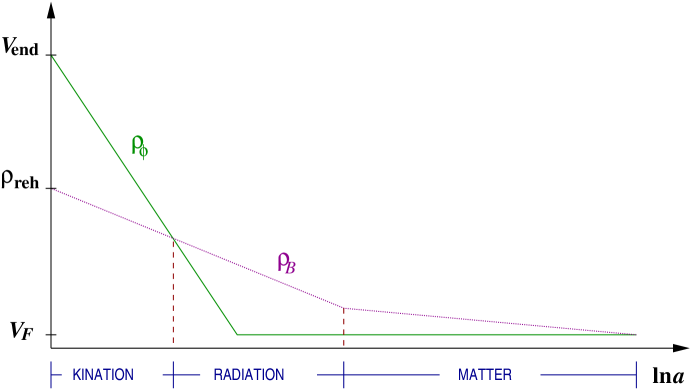
Figure 1: The scaling of $\rho_{\phi}$ (solid line) and $\rho_{B}$ (dotted line) after the end of inflation. Initially, $\rho_{\phi}=V_{\rm end}\gg\rho_{\rm reh}=\rho_{B}$ and we have kination. However, because $\rho_{\phi}=\rho_{\rm kin}\propto a^{-6}$, whereas $\rho_{B}=\rho_{\gamma}\propto a^{-4}$, eventually $\rho_{B}$ dominates $\rho_{\phi}$ and kination ends. Afterwards $\rho_{\phi}$ continues to be $\rho_{\rm kin}$–dominated until all the kinetic energy is depleted and the field freezes at constant density $\rho_{\phi}=V_{F}$. In the meantime the radiation era continues and $\rho_{B}=\rho_{\gamma}\propto a^{-4}$. Much later, though, matter density takes over and the radiation era ends. In the matter era $\rho_{B}=\rho_{m}\propto a^{-3}$. The matter era continues until today when $\rho_{B}\simeq V_{F}\simeq\rho_{0}$ and the scalar field becomes important again.

5 Coincidence versus BBN and Gravitational Waves

We now investigate the requirement of successful coincidence in combination with the BBN constraint in both brane and conventional cosmology. These two requirements are the most difficult to achieve in quintessential inflation. This is because, one the one hand the BBN constraint pushes the inflationary scale towards high energies, while on the other hand the coincidence constraint demands the late-time potential density of the scalar field to be extremely small. This huge difference of energy scales (of order ${\cal O}(10^{100})$!) is the basis for the $\eta$-problem of quintessential inflation.

5.1 The $\eta$-problem of quintessential inflation

In conventional cosmology, in order for inflation to last enough e-foldings to account for the horizon problem without an initially super-Planckian $V^{1/4}$, it is necessary for the potential to be rather flat during inflation. As a result, in order to prepare for the abysmal “dive” after the end of inflation (so as to cover the huge difference of energy scales) the curvature $V^{\prime\prime}$ of the potential near the end of inflation is substantial. As a result the spectral index $n_{s}$ of the inflation–generated density perturbation spectrum is too large compared with the observational requirement:

$$|n_{s}-1|\leq 0.1$$ (44)

This can be understood from the fact that $n_{s}$ is given by [5]

$$n_{s}=1+2(\eta-3\epsilon)$$ (45)

where $\eta$ and $\epsilon$ are the so–called slow roll parameters of inflation, which, in conventional cosmology, are defined as

$$\epsilon\equiv-\frac{\dot{H}}{H^{2}}\simeq\frac{m_{P}^{2}}{2}\left(\frac{V^{\prime}}{V}\right)^{2} \qquad{\rm and}\qquad \eta\equiv m_{P}^{2}\frac{V^{\prime\prime}}{V}$$ (46)

Therefore, a strongly curved potential results in unacceptably large $|\eta|$, which, in turn, because of (45), causes deviations from scale invariance that are incompatible with observations. An illustration of the $\eta$-problem can be seen in Figure 2.

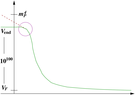
Figure 2: Graphic illustration of the source of the $\eta$-problem of quintessential inflation. In order to bridge the huge gap between the energy scales corresponding to the inflationary plateau and the quintessential tail the curvature of the potential near the end of inflation is too large to allow for an almost scale invariant spectrum of curvature perturbations. An attempt to steepen the inflationary plateau, however, would reduce the total number of inflationary e-foldings below the necessary amount required for the solution of the horizon problem, unless the inflationary scale was allowed to superseded the Planck scale.

The hope had been that brane-cosmology, since it allows overdamped steep inflation, would be able to avoid a strongly curved inflationary potential without introducing super-Planckian densities. This is because, as evident by (8), for energies above the brane tension $\lambda$, the Hubble parameter is larger than in the usual FRW case. This introduces extra friction in the roll–down of the scalar field, as determined by (3). Consequently, the roll becomes much slower and, even with sufficiently large number of inflationary e-foldings to solve the horizon problem, the field rolls so little that super-Planckian densities can be avoided. Moreover, slow-roll can be achieved even when dispensing with the inflationary plateau, leading to the so–called steep inflation [23], which again assists in reducing the curvature of the potential during inflation.

5.2 Coincidence and BBN

However, as we show below, the above beneficial effects of brane-cosmology are counteracted by the consequences of extra friction in the period of kination. Indeed, overdamped kination is reduced in duration. As a result, the field is not able to roll as much down its quintessential tail as it would in conventional cosmology, which intensifies the already stringent constraints of coincidence and BBN. To demonstrate this in a quantified way, we study below these constrains considering an exponential quintessential tail of the form:

$$V(\phi)=V_{\rm end}\exp(-b\Delta\phi/m_{P})$$ (47)

where $\Delta\phi\equiv\phi-\phi_{\rm end}$. Using (32) the coincidence requirement (43) results in the constraint:

$$\begin{array}[]{l}\left(1\!+\!\sqrt{\frac{3}{2}}\,b\right)\ln\!\Big{(}\mbox{\large$\frac{m_{P}^{4}}{V_{\rm end}}$}\Big{)}\mbox{=}\ln\!\Big{(}\mbox{\large$\frac{m_{P}^{4}}{\rho_{0}}$}\Big{)}\mbox{-}\ln\Omega_{\phi}\,\mbox{-}\sqrt{\frac{3}{2}}\,b\!\left[\frac{8}{3}\!+\!2\ln\!\left(\!\frac{48\pi}{\alpha^{2}}\!\sqrt{\frac{30}{g_{\rm reh}}}\right)\mbox{-}\frac{4}{3}\sqrt{\mbox{\large$\frac{\lambda}{2V_{\rm end}}$}}\,\mbox{-}\frac{7}{3}\ln\!\left(\mbox{\large$\frac{2V_{\rm end}}{\lambda}$}\right)\right]\end{array}$$ (48)

Similarly, the requirement $T_{*}>T_{\sc bbn}$, in view of (24), becomes

$$\ln\!\left(\frac{m_{P}^{4}}{V_{\rm end}}\right)\leq\ln\!\left[\frac{\alpha^{3}}{(24\pi)^{2}}\sqrt{\frac{g_{\rm reh}}{10}}\left(\frac{g_{\rm reh}}{g_{*}}\right)^{1/4}\right]+\frac{3}{2}\ln\!\left(\frac{2V_{\rm end}}{\lambda}\right)+\ln\!\left(\frac{m_{P}}{T_{\sc bbn}}\right)$$ (49)

Combining the above one finds the bound: $b\geq b_{\rm min}$, where

$$b_{\rm min}\equiv\sqrt{\frac{2}{3}}\;\;\frac{\ln\!\Big{(}\mbox{\large$\frac{m_{P}^{4}}{\rho_{0}}$}\Big{)}-\ln\Omega_{\phi}-\ln\!\left[\mbox{\large$\frac{\alpha^{3}}{(24\pi)^{2}}$}\sqrt{\mbox{\large$\frac{g_{\rm reh}}{10}$}}\left(\mbox{\large$\frac{g_{\rm reh}}{g_{*}}$}\right)^{1/4}\right]-\ln\!\left(\mbox{\large$\frac{m_{P}}{T_{\sc bbn}}$}\right)-\mbox{\large$\frac{3}{2}$}\ln\!\left(\mbox{\large$\frac{2V_{\rm end}}{\lambda}$}\right)}{\ln\!\left[\mbox{\large$\frac{12}{\alpha}$}\sqrt{\mbox{\large$\frac{10}{g_{\rm reh}}$}}\left(\mbox{\large$\frac{g_{\rm reh}}{g_{*}}$}\right)^{1/4}\right]+\mbox{\large$\frac{8}{3}$}+\ln\!\left(\mbox{\large$\frac{m_{P}}{T_{\sc bbn}}$}\right)-\mbox{\large$\frac{4}{3}$}\sqrt{\mbox{\large$\frac{\lambda}{2V_{\rm end}}$}}-\mbox{\large$\frac{5}{6}$}\ln\!\left(\mbox{\large$\frac{2V_{\rm end}}{\lambda}$}\right)}$$ (50)

The above expression looks rather complicated but, in fact, it becomes quite simple once the numbers are introduced. We are going to use $g_{*}=10.75$ and $g_{\rm reh}=106.75c$, where $c=1$ for the SM and $c\mbox{\raisebox{-3.87495pt}{~{}$\stackrel{{\scriptstyle\mbox{$>$}}}{{\sim}}$~{}}}2$ for its supersymmetric extensions. Also, in order to compensate for the overestimate of $T_{*}$ in (24), we will use $T_{\sc bbn}\simeq 10$ MeV. Finally, let us define: $Y\equiv\ln(2V_{\rm end}/\lambda)$. Then we find

$$b_{\rm min}=\sqrt{\frac{2}{3}}\;\frac{236.66-\frac{3}{4}\ln c-3\ln\alpha-\frac{3}{2}Y}{51.48-\frac{1}{4}\ln c-\ln\alpha-\frac{4}{3}e^{-Y/2}-\frac{5}{6}Y}$$ (51)

Thus we see that $b_{\rm min}$ grows with $Y$, which means that the more prominent the brane effect becomes the more the parameter space for $b$ shrinks. Indeed, remember that, from (42), the maximum acceptable value of $b$, in order for brief acceleration to occur, is $b_{\rm max}=2\sqrt{6}$.

Thus, as far as kination and BBN are concerned, the case of conventional cosmology is preferable. We can recover conventional cosmology if we set $Y=0$ and $\alpha\rightarrow 2\alpha$. This gives

$$b_{\rm min}=\sqrt{\frac{2}{3}}\;\frac{234.58-\frac{3}{4}\ln c-3\ln\alpha}{49.46-\frac{1}{4}\ln c-\ln\alpha}$$ (52)

The lowest value for the above corresponds to $c=1$ and $\alpha\simeq 0.1$, for which we find $b_{\rm min}=3.81$. Note that, in both conventional and brane cosmology, $b_{\rm min}>b_{\rm min}(\alpha\rightarrow 0)=\sqrt{6}$. According to [33], when $b\geq\sqrt{6}$ the attractor (35) is unreachable. Instead, after unfreezing the field engages again in free-fall evolution, where $\rho_{\phi}\simeq\rho_{\rm kin}\propto a^{-6}$, until it refreezes at another value $\phi_{F^{\prime}}=\phi_{F}+\sqrt{2V_{F}}\,t_{F}$, where $t_{F}$ is the time of unfreezing. This is true regardless of $w_{B}$ as can be shown easily through the use of (14). Using (5) we find

$$\phi_{F^{\prime}}=\phi_{F}+\frac{4}{\sqrt{6}(1+w_{B})}\,m_{P}$$ (53)

The process can be repeated again and again, leading to many ‘glitches’ of brief accelerated expansion. This effect may enlarge the parameter space since it is expected to relax the coincidence constraint because the final value of $V$ today can be lower than $V_{F}$. This possibility certainly deserves further investigation, which, however, we will not pursue here. An illustration of this process is shown in Figure 3.

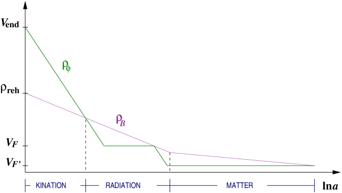
Figure 3: The evolution of $\rho_{\phi}$ (solid line) and $\rho_{B}$ (dotted line) in the multiple–unfreezings scenario. For $b\geq\sqrt{6}$, after unfreezing from $V_{F}$ the field engages again into free fall until its kinetic energy is depleted once more, when it freezes again at a new position with potential density $V_{F^{\prime}}\equiv V(\phi_{F^{\prime}})\ll V_{F}$. The process may be repeated many times. Each unfreezing stage causes a brief period of accelerated expansion for the Universe and also sends $\phi$ further down its potential so that coincidence becomes easier to achieve.

5.3 Gravitational waves

Another important constraint related to the kination period has to do with the spectrum of the Gravitational Waves (GW) generated during inflation. Because of the stiffness of the equation of state of the Universe, the GW spectrum forms a spike at high frequencies, instead of being flat as is the case for the radiation era [34]. Indeed, it has been shown that the GW spectrum is of the form [34][35]:

$$\Omega_{\sc gw}(k)=\left\{\begin{array}[]{ll}\varepsilon\Omega_{\gamma}(k_{0})h_{\sc gw}^{2}\left(\mbox{\large$\frac{k}{k_{*}}$}\right)[\ln(k/k_{\rm end})]^{2}&k_{*}<k\leq k_{\rm end}\\ &\\ \frac{\pi}{4}\varepsilon\Omega_{\gamma}(k_{0})h_{\sc gw}^{2}[\ln(k_{*}/k_{\rm end})]^{2}&k_{\rm eq}<k\leq k_{*}\\ &\\ \frac{\pi}{16}\varepsilon\Omega_{\gamma}(k_{0})h_{\sc gw}^{2}\left(\mbox{\large$\frac{k_{\rm eq}}{k}$}\right)^{2}[\ln(k_{*}/k_{\rm end})]^{2}&k_{0}<k\leq k_{\rm eq}\end{array}\right.$$ (54)

where $\Omega_{\sc gw}(k)$ is the density fraction of the gravitational waves with physical momentum $k$, $\Omega_{\gamma}(k_{0})=2.6\times 10^{-5}h^{-2}$ is the density fraction of radiation at present on horizon scales ($h=0.65$ is the Hubble constant $H_{0}$ in units of 100 km/sec/Mpc) and the subscripts ‘$*$’ and ‘eq’ denote the end of kination (onset of radiation era) and the end of radiation era (onset of matter era) respectively. Moreover, $\varepsilon=\alpha_{\sc gw}/2\pi\sim 10^{-2}$ with $\alpha_{\sc gw}\sim 0.1$ being the GW generation efficiency during inflation and [35][36]

$$h_{\sc gw}\equiv\frac{1}{\pi}\left(\frac{H_{\rm end}}{m_{P}}\right){\cal F}(\rho/\lambda)$$ (55)

where [36]

$${\cal F}(x)\equiv\left[\sqrt{1+x^{2}}-x^{2}\ln\left(\frac{1}{x}+\sqrt{1+\frac{1}{x^{2}}}\right)\right]^{-1/2}\!\!\Rightarrow\;{\cal F}(\rho/\lambda)\simeq\left\{\begin{array}[]{ll}1&\rho\ll\lambda\\ \sqrt{\frac{3}{2}(\rho/\lambda)}&\rho\gg\lambda\end{array}\right.$$ (56)

The danger is that the generated GWs may destabilize BBN. The relevant constraint on $\Omega_{\sc gw}(k)$ reeds:

$$I\equiv h^{2}\int_{k_{\sc bbn}}^{k_{\rm end}}\Omega_{\sc gw}(k)\;d\ln k\leq 2\times 10^{-6}$$ (57)

where $k_{\sc bbn}$ is the physical momentum that corresponds to the horizon at BBN. From (54) it is easy to find

$$I=h^{2}\varepsilon\Omega_{\gamma}(k_{0})h_{\sc gw}^{2}\left\{2\left(\frac{k_{\rm end}}{k_{*}}\right)-\left[\ln\left(\frac{k_{\rm end}}{k_{*}}\right)+1\right]^{2}+\frac{\pi}{4}\left[\ln\left(\frac{k_{\rm end}}{k_{*}}\right)\right]^{2}\ln\left(\frac{k_{*}}{k_{\sc bbn}}\right)\right\}$$ (58)

Since $k_{\rm end}\gg k_{*}>k_{\sc bbn}$ the expression in brackets above is dominated by the first term. We also have

$$\frac{k_{\rm end}}{k_{*}}=\frac{H_{\rm end}}{H_{*}}\left(\frac{a_{\rm end}}{a_{*}}\right)=\left(\frac{H_{\rm end}}{H_{*}}\right)^{2/3}\left(\frac{H_{\rm end}}{H_{\lambda}}\right)^{1/6}$$ (59)

where $H_{\lambda}\equiv H(t_{\lambda})$ and the last factor reduces to unity when considering conventional kination. Putting all these together we find

$$I=2h^{2}\varepsilon\Omega_{\gamma}(k_{0})h_{\sc gw}^{2}\left(\frac{H_{\rm end}}{H_{*}}\right)^{2/3}\left(\frac{H_{\rm end}}{H_{\lambda}}\right)^{1/6}$$ (60)

Inserting the above into (57) and after some algebra we end up with the constraint:

$$\alpha^{4}\geq\frac{15}{g_{\rm reh}}\frac{\lambda{\cal F}^{2}(V_{\rm end}/\lambda)}{(m_{P}H_{\rm end})^{2}}\left(\frac{2V_{\rm end}}{\lambda}\right)^{3/2}$$ (61)

In the case of brane cosmology we have ${\cal F}^{2}\simeq\frac{3}{2}(V_{\rm end}/\lambda)$ so that the bound becomes

$$\alpha\mbox{\raisebox{-3.87495pt}{~{}$\stackrel{{\scriptstyle\mbox{$>$}}}{{\sim}}$~{}}}\left(\frac{270}{g_{\rm reh}}\right)^{1/4}\left(\frac{2V_{\rm end}}{\lambda}\right)^{1/8}$$ (62)

whereas for conventional cosmology ${\cal F}^{2}\simeq 1$ and the bound is

$$\alpha\mbox{\raisebox{-3.87495pt}{~{}$\stackrel{{\scriptstyle\mbox{$>$}}}{{\sim}}$~{}}}\left(\frac{90}{g_{\rm reh}}\right)^{1/4}$$ (63)

Thus, we see that the brane-effect also sets a somewhat tighter lower bound on the reheating efficiency due to excessive GW generation. In both cases $\alpha\mbox{\raisebox{-3.87495pt}{~{}$\stackrel{{\scriptstyle\mbox{$>$}}}{{\sim}}$~{}}}1$ and, therefore, purely gravitational reheating is only marginally compatible with the GW constraint.

Here, we should mention another, potentially more dangerous relic, introduced by gravitational reheating, namely gravitinos. Gravitino overproduction is also possible to endanger BBN. In fact they are rather stringently constrained as [37]

$$\frac{n_{g}}{s}\leq 10^{-14}$$ (64)

where $n_{g}$ is the number density of the gravitinos which is kept in constant ratio with the entropy $s$ of the Universe. The above ratio is easy to compute [4]:

$$\frac{n_{g}}{s}=\frac{135\zeta(3)}{2\pi^{4}g_{\rm reh}}\left(\frac{\alpha_{g}}{\alpha}\right)^{3}$$ (65)

where $\zeta(3)=1.20206$ and $\alpha_{g}$ is the production efficiency of gravitinos. The above provide the following lower bound on the reheating efficiency:

$$\alpha\geq 9\times 10^{3}c^{-1/3}\alpha_{g}$$ (66)

According to [37] gravitino production can be as efficient as the gravitational production of any other particle, i.e. $\alpha_{g}\sim 0.1$, even though the gravitinos are not generated during inflation but only afterwards (that is at the end of inflation). Indeed, the gravitino overproduction danger concerns the spin-$\frac{1}{2}$ gravitinos and not the usual spin-$\frac{3}{2}$ ones. The spin-$\frac{1}{2}$ gravitinos (longitudinal modes) are massive because they absorb the goldstino mode and this is why they cannot be generated during inflation. Still, to date there is no thorough calculation of $\alpha_{g}$ in a stiff equation of state and also in the case of brane–cosmology so, the gravitino bound (66) may not be as reliable as the bounds due to GW generation.

In a similar way as described above, the stiff equation of state during kination may lead to efficient production of supersymmetric dark matter, e.g. neutralinos [38]. Moreover, the fluctuations of the inflaton field itself can be considered as dark matter [39]. Finally, if the rolling scalar field is even weakly coupled to SM fields it may lead to substantial leptogenesis or baryogenesis even though the Universe is in thermal equilibrium, which may explain the observed baryon asymmetry [40]. It has been shown that the backreaction of the latter effect does not affect the dynamics of $\phi$ and (3) is still valid.

6 The curvaton hypothesis

As we have shown in the previous section, even though brane cosmology may help with the $\eta$-problem by allowing overdamped steep inflation, it is this very effect of overdamping that turns negative during kination by making it harder for the field to roll down enough so as to achieve successful coincidence. Is, then, all lost for quintessential inflation?

Fortunately it is not. An alternative way to ameliorate the $\eta$-problem is through the so–called curvaton hypothesis [24]. According to this hypothesis the curvature perturbation spectrum, which seeds the formation of Large Scale Structure and the observed anisotropy of the Cosmic Microwave Background Radiation (CMBR), is due to the amplification of the quantum fluctuations of a scalar field other than the inflaton during inflation. This field $\sigma$, called curvaton, has to satisfy certain requirements to fulfill its role in generating the correct curvature perturbation spectrum. In order for its quantum fluctuations to get amplified during inflation the curvaton $\sigma$, much like the inflaton in conventional inflation, has to be an effectively massless scalar field, with mass $m_{\sigma}<\frac{3}{2}\,H_{\rm inf}$, where $H_{\rm inf}$ is the Hubble parameter during inflation. Also, in order for the generated perturbations to be Gaussian, in accordance to observations, the curvaton should be significantly displaced from its vacuum expectation value (VEV) during inflation, i.e. $|\sigma-\langle\sigma\rangle|\gg H_{\rm inf}$. However, the curvaton’s contribution to the potential density during inflation is negligible and this is why inflationary dynamics is still governed by the inflaton field. One final requirement for a successful curvaton field is that its couplings to the reheated thermal bath are small enough to prevent its thermalization after the end of inflation (which would, otherwise, wipe out its superhorizon perturbation spectrum).

The curvaton, being subdominant and effectively massless during inflation remains overdamped and, more or less, frozen. After the end of inflation $\sigma$ remains frozen until $H(t)\sim m_{\sigma}$, when the field unfreezes and begins oscillating around its VEV. Doing so its average energy density scales as pressureless matter, i.e. $\rho_{\sigma}\propto a^{-3}$. This means that, if the unfreezing of the curvaton occurs early enough (i.e. before the matter era) the latter comes to dominate the Universe, causing a brief period of matter domination, until it decays into a new thermal bath comprised by the curvaton’s decay products. This is expected to somewhat relax the GW and gravitino constraints because the additional entropy production by the decay of the curvaton will dilute the GW/gravitino contribution to the overall density. The curvature perturbation spectrum of $\sigma$ is imposed onto the Universe, when the latter becomes curvaton dominated (or nearly dominated).

There are two important differences between the curvaton hypothesis and conventional inflation. Firstly, because the curvature perturbation spectrum is due to the curvaton the spectral index is not given by (45) but by [24]

$$n_{s}=1+2(\eta_{\sigma\sigma}-\epsilon\,)$$ (67)

where

$$\eta_{\sigma\sigma}\equiv\frac{m_{P}^{2}}{V}\frac{\partial^{2}V}{\partial\sigma^{2}}$$ (68)

Now, since the $\sigma$-dependent part of $V$ is not related to inflation $\eta_{\sigma\sigma}$ can be extremely small. This means that the spectral index constraint (44) becomes

$$\epsilon<0.05$$ (69)

which is possible to satisfy even for large $\eta$ and much easier too. Thus, the $\eta$-problem for quintessential inflationary model building is ameliorated through the curvaton hypothesis because one can keep an almost scale invariant spectrum of curvature perturbations even with a substantially curved scalar potential.

The second effect of the curvaton hypothesis on inflationary model building is the fact that the cobe observations impose only an upper bound on the amplitude of the inflaton generated curvature perturbations. If we want to allow for a large $\eta$ then this bound should be

$$\frac{1}{2\pi}\left.\frac{\delta\phi}{\phi}\right|_{\rm exit}\leq 0.1\left(\frac{\Delta T}{T}\right)_{\sc cobe}\simeq 5\times 10^{-6}$$ (70)

which, for slow roll inflation, can be recast as

$$\frac{1}{\sqrt{3}\pi}\frac{V^{3/2}}{m_{P}^{3}|V^{\prime}|}\leq 10^{-5}$$ (71)

There are numerous candidates for successful curvatons, especially in supersymmetric theories, where scalar fields are abundant. Of particular interest are pseudo-Goldstone bosons or axion-like string moduli, because their mass is protected by symmetries and can be rather small during inflation. In [25] the liberation effect of the curvaton hypothesis on inflationary model building has been shown by demonstrating how it can rescue a number of, otherwise unviable inflationary models, which are well motivated by particle physics.

In the following sections we will apply the curvaton hypothesis on quintessential inflation model building both in conventional and brane cosmology, demonstrating thereby the fact that the $\eta$-problem is, indeed, substantially ameliorated.

7 The case of Standard Cosmology

Let us first consider the case of conventional cosmology, where kination is not inhibited by overdamping effects. We focus on modular inflation which has the merit that the scalar field is a modulus, which corresponds to a flat direction protected from excessive supergravity corrections and may refrain from steepness even when the field travels distances as large as $m_{P}$ in field space, a problem which, in most models of quintessence, is unresolved [9].

7.1 Modular inflation

Moduli fields correspond to flat directions in field space that are protected by symmetries against supergravity corrections. However, the values of string-inspired moduli are typically related to observables, such as the gauge coupling in the case of the dilaton, and need to become stabilized. This is usually supposed to occur at inner-space distances of order $m_{P}$, where non-perturbative Kähler corrections may generate a minimum for the field. Thus, the expected VEV for a modulus is $\langle\phi\rangle\sim m_{P}$. Therefore, the scalar potential for a modulus near its origin would be

$$V(\phi)=V_{0}-\frac{1}{2}m^{2}\phi^{2}+\cdots$$ (72)

where, $V$ is expected to depart from $V_{0}$ when $\delta\phi\sim m_{P}$, so that

$$V_{0}\sim(m_{P}m)^{2}$$ (73)

The inflationary scale is usually taken to be the so–called intermediate scale $V_{0}^{1/4}\simeq 5\times 10^{10}$ corresponding to gravity mediated supersymmetry breaking. Then, from the above $m\sim 1$ TeV. As a result we find

$$|\eta|=\frac{(m_{P}m)^{2}}{V_{0}}\sim 1$$ (74)

which means that such a modulus field cannot be the inflaton of conventional inflation because it would be impossible to attain a scale invariant spectrum of curvature perturbations. Moreover, the inflationary energy scale is too low to generate the necessary amplitude for the curvature perturbations.

In contrast, as shown in [25], modular inflation works fine in the context of the curvaton hypothesis. Indeed, from (72), it is easy to see that

$$\epsilon=\frac{\eta^{2}}{2}\left(\frac{\phi}{m_{P}}\right)^{2}$$ (75)

which can become very small near the origin and easily satisfy the constraint (69). The question is, of course, why should $\phi$, stand at the origin in the first place. This is natural to occur if the origin is point of enhanced symmetry [41], where the modulus field has strong couplings with the fields of some thermal bath preexisting inflation. Such strong couplings introduce temperature corrections to (72) which drive $\phi$ to zero. The inflationary expansion, then, begins with a period of thermal inflation, which inflates away the primordial thermal bath and renders the origin a local maximum. Afterwards, quantum fluctuations send the field rolling down and away from the origin, in a period of fast-roll inflation. This model, called thermal modular inflation, is discussed in [25].

It is possible to formulate a model of quintessential inflation based on modular inflation if one considers that the supergravity corrections introduced into the potential at $\phi\sim m_{P}$ may not generate a minimum for the potential but just give rise to a slope, with the minimum displaced at infinity. After all, for the moduli one only expects that $\delta V(\delta\phi\sim m_{P})\sim V$. Thus, for example, the potential may look like this

$$V(\phi)\simeq\left\{\begin{array}[]{lc}V_{0}-\frac{1}{2}m^{2}\phi^{2}&0<\phi\ll m_{P}\\ &\\ V_{0}\exp(-b\phi/m_{P})&\phi\gg m_{P}\end{array}\right.$$ (76)

This form is rather plausible for moduli potentials. Indeed, the $F$-term scalar potential in supergravity is

$$V\simeq e^{K/m_{P}^{2}}|W|^{2}\left[\sum_{nm}\left(\frac{K_{n}}{m_{P}^{2}}+\frac{W_{n}}{W}\right)K^{nm}\left(\frac{K_{m}}{m_{P}^{2}}+\frac{\bar{W}_{m}}{\bar{W}}\right)-3\,m_{P}^{-2}\right]$$ (77)

where $W$ is the superpotential, $K$ is the Kähler potential, $K^{nm}=(K_{nm})^{-1}$, the overbar denotes charge conjugation and the subindices represent derivatives with respect to the different fields of the theory. In many string models the dynamics of the above is dominated by the $e^{K/m_{P}^{2}}$ factor (see for example [42]). Now, the Kähler potential, at tree level, is logarithmic with respect to the moduli $\Phi_{i}$ such that $K\propto-m_{P}^{2}\sum_{i}\ln[(\Phi_{i}+\bar{\Phi}_{i})/m_{P}]$, which means that $e^{K/m_{P}^{2}}\propto 1/\prod_{i}[(\Phi_{i}+\bar{\Phi}_{i})/m_{P}]$. Note that the $\Phi_{i}$ moduli do not have canonical kinetic terms. Instead the kinetic part of the relevant Lagrangian density is given by

$${\cal L}_{\rm kin}=K_{ij}\;\partial_{\mu}\Phi_{i}\partial^{\mu}\bar{\Phi}_{j}$$ (78)

which means that we can define the canonically normalized moduli as $\phi_{i}\propto\ln[(\Phi_{i}+\bar{\Phi}_{i})/m_{P}]$, in terms of which the scalar potential becomes an exponential, i.e. $V\propto\exp(-\sum_{i}b_{i}\phi_{i}/m_{P})$. the values of the positive $b_{i}$ coefficients in the exponents depend on the particular string model considered but, in general they are of order unity (for example in [42] $b=2\sqrt{2}$ whereas in [44] $b=4\sqrt{\pi}$). Obviously, the potential is eventually dominated by the term with the smallest $b_{i}$.

The potential can easily form a maximum at the origin if there exists a discrete symmetry of the form $\phi_{i}\rightarrow-\phi_{i}$ (which corresponds to the well known $T$-duality: $e^{\phi_{i}}=1/e^{\phi_{i}}$). In this case the couplings of the moduli with matter at the origin are maximized [43], exactly as required by thermal modular inflation. In contrast, away from the origin, these couplings are strongly suppressed leading to an effectively sterile inflaton, as required by quintessential inflation.

It is important to note that in the case described above the modulus is not stabilized by reaching its VEV, but it does so dynamically, when reaching $\phi=\phi_{F}$ where it freezes. Of course $\phi_{F}$ has to be at the correct value for phenomenology to work. This is especially true for the dilaton, which determines the gauge coupling. Thus, it would be safer to consider the so-called geometrical moduli ($T$-moduli) associated with the volume of the extra dimensions. The dependence of the SM–phenomenology on these is not manifest at tree-level but arises only at one-loop and beyond.

The above are based on the implicit assumption that the superpotential has only a weak dependence on the moduli and, therefore, $V$ is mostly determined by the $e^{K/m_{P}^{2}}$ factor. However, it should be pointed out here that, according to the usual interpretation of (heterotic) string phenomenology, the superpotential receives non-perturbative contributions from hidden sector gaugino condensates, which are of the form $W\propto\exp(-\sum_{i}\beta_{i}\Phi_{i}/m_{P})$. Consequently, a $T$-modulus would have a double exponential potential. As discussed in [13], such a potential, being steeper than the pure exponential, has a disastrous attractor solution. Indeed, not only does this attractor diminish $\rho_{\phi}$ much faster than $\rho_{B}$ but it is also attained very soon after the end of inflation and, therefore, renders late-time $\phi$-domination impossible. However, not all the possibilities for the moduli have been explored and there are more types of string theory than the usual heterotic string. So, we believe that it is quite possible that a canonically normalized modulus may have a scalar potential with the desired pure exponential tail.

Below we will examine the bahavour of a toy model that bares the characteristics outlined above and investigate whether it is indeed possible to be a successful quintessential inflationary model. We name this proposal modular quintessential inflation.

7.2 Modular quintessential inflation

7.2.1 The toy model

Consider the potential:

$$V(\phi)=\frac{M^{4}}{[\cosh(\phi/m_{0})]^{q}}$$ (79)

where $q$ is a positive integer and $M,m_{0}$ are mass scales. The above becomes

$$V(\phi)\simeq\left\{\begin{array}[]{lc}M^{4}-\frac{1}{2}q(M^{2}/m_{0})^{2}\phi^{2}&\qquad 0<\phi\ll m_{P}\\ &\\ 2^{q}M^{4}\exp(-q\phi/m_{0})&\qquad\phi\gg m_{P}\end{array}\right.$$ (80)

which can be identified with (76) if we define:

$$m^{2}\equiv q\,\frac{M^{4}}{m_{0}^{2}} \qquad V_{0}\equiv M^{4}\qquad b\equiv q\,\frac{m_{P}}{m_{0}}$$ (81)

The slow roll parameters for the above model are

$$\epsilon=\frac{1}{2}\,b^{2}[\tanh(\phi/m_{0})]^{2} \eta=2\epsilon-\frac{b^{2}}{q}[\cosh(\phi/m_{0})]^{-2}$$ (82)

In order to have enough e-foldings of inflation we need $\eta(\phi\rightarrow 0)\geq-1$, which demands $q\geq b^{2}$. Then it can be shown that inflation ends at

$$\phi_{\rm end}\simeq\sqrt{\frac{2}{|\eta|}}\,m_{P}\simeq\frac{\sqrt{2q}}{b}\,m_{P}$$ (83)

The number of fast-roll e-foldings before the end of inflation is related to the value of the scalar field at that time $\phi_{N}$ by [45]

$$N\simeq\frac{1}{F}\ln\left(\frac{\phi_{\rm end}}{\phi_{N}}\right)\Rightarrow\phi_{N}=\phi_{\rm end}\exp(-FN)$$ (84)

where

$$F\equiv\frac{3}{2}\left(\sqrt{1+\frac{4}{3}|\eta|}-1\right)$$ (85)

which, for slow roll inflation, becomes $F(|\eta|\ll 1)\approx|\eta|$.

7.2.2 Enforcing the constraints

Let us employ now the cobe bound (71). We find that the bound translates into a lower bound on $q$ such that $q\geq q_{\rm min}$, where

$$q_{\rm min}\equiv\frac{b^{2}N_{\rm dec}}{2\mu-5\ln 10+\frac{1}{2}\ln(6\pi^{2}/q_{\rm min})+\ln b}$$ (86)

In the above we have defined $\mu\equiv\ln(m_{P}/M)$ and also $N_{\rm dec}$ is the number of inflationary e-foldings that remain when the scale, which reenters the horizon at decoupling (corresponding to the time of emission of the CMBR), exits the horizon during inflation. This scale is related to the reheating efficiency by [13]

$$N_{\rm dec}=\ln(T_{\sc cmb}t_{0})+\ln(H_{\rm end}/T_{\rm reh})=66.94-\ln\alpha$$ (87)

where $T_{\sc cmb}$ is the temperature of the CMBR at the present time $t_{0}$.

Let us now enforce the coincidence constraint (48) in the case of conventional cosmology ($\lambda=2V_{\rm end}$ and $\alpha\rightarrow 2\alpha$). With a little algebra we find

$$b=\sqrt{\frac{2}{3}}\frac{69.18-\mu}{1.83-\frac{1}{4}\ln c-\ln\alpha+\mu}$$ (88)

which diminishes with $\mu$ and, therefore, we can define $\mu_{\rm min}\equiv\mu(b_{\rm max})$, where, according to (42), $b_{\rm max}=2\sqrt{6}$. Thus, we obtain

$$\mu_{\rm min}=8.31+\frac{3}{14}\ln c+\frac{6}{7}\ln\alpha$$ (89)

Finally, let us use the BBN constraint (49) to obtain the upper bound on $\mu$. Similarly as above we find

$$\mu_{\rm max}=10.53+\frac{3}{16}\ln c+\frac{3}{4}\ln\alpha$$ (90)

Both $\mu_{\rm min}$ and $\mu_{\rm max}$ increase with $\alpha$, but with different rates so that the $\mu$-range decreases. Thus there is an upper bound on $\alpha$ where $\mu_{\rm min}=\mu_{\rm max}$. It is easy to see that

$$\ln\alpha_{\rm max}=20.72-\frac{1}{4}\ln c\Rightarrow\alpha_{\rm max}\approx 10^{9}c^{-1/4}$$ (91)

The lower bound on the reheating efficiency is set by the GW constraint (63). Therefore, the $\alpha$-range is

$$1\leq\alpha\leq 10^{9}$$ (92)

It can be checked that even $\alpha_{\rm max}$ is much smaller that the reheating efficiency $\alpha_{\rm pr}$, which corresponds to prompt reheating: $\rho_{\rm reh}(\alpha_{\rm pr})=V_{\rm end}$. Note, however, that the gravitino bound (66) can chop off the lowest part of the above range by about a couple of orders of magnitude if it is not efficiently diluted by the curvaton decay.

From (89) and (90) we find the following range for the inflationary scale for a given $\alpha$

$$6.5\times 10^{13}c^{-3/16}\alpha^{-3/4}{\rm GeV}\leq M\leq 6.0\times 10^{14}c^{-3/14}\alpha^{-6/7}{\rm GeV}$$ (93)

which is shown in Figure 4. We see that entirely uncorrelated physics (BBN and coincidence requirements) conspires to allow only a rather narrow range for $M$. The range ends up at $\alpha_{\rm max}$, which corresponds to the smallest possible value for $M$, which is

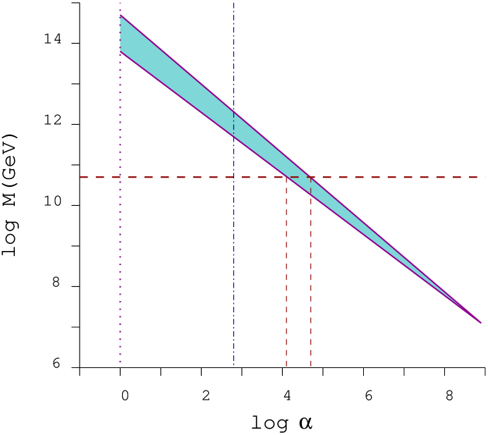
Figure 4: The shaded region depicts the allowed parameter space for the inflationary scale $M$. The parameter space is bounded from below by the requirements of BBN and from above by the cobe bound (solid lines). The bounds meet at $\alpha\simeq 10^{10}$, which corresponds to $M_{\sc min}\simeq 10^{7}$GeV. The lower bound on $\alpha$ is set by the GW constraint which results in $\alpha\geq 1$ (dotted line). The dashed horizontal line depicts the case of modular quintessential inflation, for which $M=5\times 10^{10}$GeV. The vertical dashed lines correspond the the $\alpha$-range for modular quintessential inflation. The vertical dashed–dotted line corresponds to the gravitino lower bound on $\alpha$, if not diluted by the curvaton’s decay.

$$M_{\sc min}=1.2\times 10^{7}{\rm GeV}$$ (94)

The fact that the curvaton hypothesis ameliorates the $\eta$-problem is related to the value of $q_{\rm min}$. In conventional inflation the cobe bound is to be saturated and $q=q_{\rm min}$. However, the spectral index bound (44), in view of (45), demands that $|\eta|\leq 1/20$, which, according to (82) requires

$$q>20\;b^{2}$$ (95)

which is impossible to satisfy with $q_{\rm min}$ in the given ranges for $b,\mu$ and $\alpha$. In contrast, the spectral index constraint (69) in the curvaton case is well satisfied in the allowed parameter space. This difference will become apparent in the examples below.

7.2.3 Examples

The modular case

In this case inflation is of the intermediate energy scale which means that $M=5\times 10^{10}$GeV. Then, using (93) one can find the allowed range for $\alpha$:

$$1.4\times 10^{4}c^{-1/4}\leq\alpha\leq 5.7\times 10^{4}c^{-1/4}$$ (96)

which is rather narrow but it is above the gravitino bound (66). Let us choose $\alpha\equiv 3\times 10^{4}c^{-1/4}$. Then, from (88) we find

$$b=4.56$$ (97)

Using the above (86) gives

$$q_{\rm min}=46$$ (98)

which is quite large but cannot be compared to the requirements of conventional inflation, which, according to (95), would demand $q\geq 416$! Thus, we see that modular quintessential inflation can be realized only in the context of the curvaton hypothesis. This is because, with $q=q_{\rm min}$, $|\eta|$ is too large to achieve the required almost-scale invariant spectrum of curvature perturbation. Therefore, the curvaton hypothesis is necessary to overcome the $\eta$-problem of quintessential inflation in conventional cosmology. Although, strictly speaking, the above results have been obtained in the context of the toy–model of (79), we believe that they are generally true for models of the type (76) because, as mentioned in Sec. 3, the dynamics of $\phi$ are oblivious to the potential during kination and, therefore, only the limits of large/small $\phi$, as depicted in (80), are important.

To obtain an estimate of all the quantities involved in the problem let us choose $q=48$ and $c\approx 2$. Then, from (81) we find

$$m_{0}=10.5\;m_{P}\approx 2\,M_{P} \quad{\rm and}\quad m=0.7\;{\rm TeV}$$ (99)

which are both rather natural. Using these we also find

$$T_{\rm reh}=2\times 10^{6}{\rm GeV} \quad{\rm and}\quad T_{*}=100\;{\rm MeV}$$ (100)

As pointed out earlier, both these values are overestimated by about an order of magnitude because of the oversimplified assumption of sudden transition from inflation to kination. Still, note that the gravitino constraint on $T_{\rm reh}$ is well satisfied, as well as the BBN constraint on $T_{*}$.

From (33) we also find,

$$\phi_{F}\simeq\left(9.01+\sqrt{q}/16.2\right)M_{P}$$ (101)

which, for $q=48$ gives $\phi_{F}\simeq 9.44\;M_{P}$. If modular quintessential inflation is indeed based on a string model, then the correct phenomenology would determine $q$ such that $\phi_{F}$ is appropriate. The above value corresponds to rather large extra dimensions and, therefore, it is not clear whether it may be accommodated in a realistic string theory.

Finally, in view of (84), the total number of fast-roll inflationary e-foldings is

$$N_{\rm tot}\simeq\frac{1}{F}\ln\left(\frac{\phi_{\rm end}}{\phi_{\rm in}}\right)$$ (102)

where $\phi_{\rm in}\simeq H_{\rm inf}/2\pi$ because the rolling phase begins after the inflaton is “kicked” away from the origin by its quantum fluctuations. Using $|\eta|\simeq b^{2}/q$ and (83) we find $N_{\rm tot}\approx 100$. This has to be compared to the number of e-foldings that correspond to the horizon at present, which, similarly to (87), is found to be [13]

$$N_{H}=69.15-\ln\alpha$$ (103)

Thus, we find $N_{H}\approx 59<N_{\rm tot}$ and the horizon problem is solved without danger of approaching super-Planckian densities during inflation.

The case of $M_{\sc min}$

As another example we consider the case with the smallest possible $q_{\rm min}$. From (86) it is evident that $q_{\rm min}$ decreases with $\mu$. Therefore, for the smallest $q_{\rm min}$ we need to consider the smallest possible value of $M$, which is given by (94). This value corresponds to $\alpha_{\rm max}$ as given by (91) and also to $b_{\rm max}$ as given by (42). Putting all these together (86) gives

$$q_{\sc min}=26$$ (104)

This should be contrasted with the conventional inflation requirement (95) which demands $q>480$! Thus, again, we see that the curvaton hypothesis is necessary to ameliorate the $\eta$-problem.

In order to obtain estimates for the quantities of the problem let us choose $q=28$ and $c\approx 2$. Then we find

$$m_{0}=5.7\;m_{P}\approx M_{P} \quad{\rm and}\quad m=51\;{\rm keV}$$ (105)

Using these we also find

$$T_{\rm reh}=4\;{\rm TeV} \quad{\rm and}\quad T_{*}=10.3\;{\rm MeV}$$ (106)

which, again, are both overestimated by an order of magnitude, but satisfy all the relevant constraints anyway. As before, using (33), we find $\phi_{F}\simeq 7.32\;M_{P}$. Finally, in a similar manner as above we find $N_{\rm tot}\approx 79$, which is larger than $N_{H}\approx 48$ as required in order to solve the horizon problem.

8 The case of Brane Cosmology

8.1 Brane inflation

We turn now our attention to the case of brane-cosmology. In this case the inflationary dynamics occurs on energy scales higher than the brane tension (otherwise there would be no difference with the conventional case). Brane inflation has been studied in [23][46]. Here we simply cite some of the necessary tools to be used in our quintessential inflationary model building.

Above the string tension scale the slow roll parameters are modified and reed

$$\epsilon\equiv\frac{m_{P}^{2}}{2}\left(\frac{V^{\prime}}{V}\right)^{2}\frac{1+V/\lambda}{(1+V/2\lambda)^{2}} \Rightarrow \epsilon\simeq 2\lambda m_{P}^{2}\frac{(V^{\prime})^{2}}{V^{3}}$$

$$\eta\equiv m_{P}^{2}\left(\frac{V^{\prime\prime}}{V}\right)\frac{1}{1+V/2\lambda} \Rightarrow \eta\simeq 2\lambda m_{P}^{2}\frac{V^{\prime\prime}}{V^{2}}$$

Similarly the cobe constraint (71) becomes

$$\frac{1}{\sqrt{3}\pi}\frac{V^{3/2}}{m_{P}^{3}|V^{\prime}|}\left(1+\frac{V}{2\lambda}\right)^{3/2}\simeq\frac{1}{2\sqrt{6}\pi}\frac{V^{3}}{\lambda^{3/2}m_{P}^{3}|V^{\prime}|}\leq 10^{-5}$$ (108)

Finally, the number of slow-roll e-foldings before the end of inflation is related to the value of the scalar field at that time $\phi_{N}$ by

$$N=\frac{1}{m_{P}^{2}}\int_{\phi_{N}}^{\phi_{\rm end}}\frac{V}{|V^{\prime}|}\left(1+\frac{V}{2\lambda}\right)d\phi\simeq\frac{1}{m_{P}^{2}}\int_{\phi_{N}}^{\phi_{\rm end}}\frac{V^{2}}{2\lambda|V^{\prime}|}d\phi$$ (109)

8.2 Exponential quintessential inflation

8.2.1 The model

It can be checked that for models of the form of (79) or even steep models such as $V(\phi)=M^{4}[\sinh(\phi/m_{0})]^{-q}$ the inflationary period already lies in the exponential branch of the potential. Thus, it is reasonable to avoid complicated models and consider a pure exponential potential:

$$V(\phi)=M^{4}\exp(-b\phi/m_{P})$$ (110)

The above is well motivated for string moduli due to the considerations of Sec. 7.1 (but without the discrete symmetry that forms the maximum for $V$). For other motivations of exponential potentials from Kaluza-Klein, scalar tensor or higher-order gravity theories see, for example, [33] and references therein.

For the model (110) the slow roll parameters are

$$\eta=\epsilon=2A\exp(b\phi/m_{P})$$ (111)

where $A\equiv b^{2}(\lambda/M^{4})$. Hence we obtain:

$$\phi_{\rm end}=\frac{1}{b}\ln(1/2A)\,m_{P}$$ (112)

and also

$$V_{\rm end}=2AM^{4}=2b^{2}\lambda$$ (113)

Then, using (109) we find

$$\phi_{N}=-\frac{1}{b}\ln[2A(N+1)]\,m_{P}$$ (114)

and

$$V(\phi_{N})=V_{\rm end}(N+1)$$ (115)

8.2.2 The constraints

Keeping $A$ a free parameter, we will attempt to constrain the string tension $\lambda$. Let us begin with the coincidence constraint (48). Defining $z\equiv\ln(m_{P}/\lambda^{1/4})$ and after some algebra we find

$$z=\frac{56.79-b(1.88-\frac{1}{4}\ln c-\ln\alpha-\frac{5}{3}\ln b)+\frac{1}{\sqrt{6}}\ln b}{\sqrt{\frac{2}{3}}+b}$$ (116)

which diminishes with $b$. Thus, we can define $z_{\rm min}=z(b_{\rm max})$. Using $b_{\rm max}=2\sqrt{6}$ we find

$$z_{\rm min}=10.713+\frac{3}{14}\ln c+\frac{6}{7}\ln\alpha$$ (117)

Similarly to the previous section the BBN constraint (49) can be used to provide an upper bound to $z$. Indeed, with a bit of algebra we obtain

$$z_{\rm max}=10.706+\frac{3}{16}\ln c+\frac{5}{4}\ln b+\frac{3}{4}\ln\alpha$$ (118)

From the above it is evident that, once more, uncorrelated physics results in a rather slim parameter space. This parameter space diminishes with $\alpha$. Thus, we can find $\alpha_{\rm max}$ by setting $z_{\rm min}=z_{\rm max}$ (or equivalently $b_{\rm min}=b_{\rm max}$ in (51), where now $Y=\ln(2b^{2})$). We find,

$$\ln\alpha_{\rm max}=18.47-\frac{1}{4}\ln c\Rightarrow\alpha_{\rm max}\approx 10^{8}c^{-1/4}$$ (119)

The lower bound on $\alpha$ is set by the GW constraint (62), which gives, $\alpha_{\rm min}\approx 1.5(b/c)^{1/4}$. Therefore, the $\alpha$-range is

$$1\leq\alpha\leq 10^{8}$$ (120)

In view of the above the acceptable range for the brane tension, for a given $\alpha$ is

$$7.5\times 10^{12}c^{-3/16}\alpha^{-3/4}{\rm GeV}\leq\lambda^{1/4}\leq 5.4\times 10^{13}c^{-3/14}\alpha^{-6/7}{\rm GeV}$$ (121)

which is shown at Figure 5. Note that this range does not differ much from (93). This is so because both are determined by the BBN and coincidence constraints on $V_{\rm end}$, which see only the exponential behaviour of the potential. The difference in the $\alpha$–range, however, is due to the modified dynamics of brane-cosmology. The parameter space is somewhat reduced in size because of the negative effect of overdamping during kination.

The smallest possible $\lambda$ corresponds to $\alpha_{\rm max}$. Using (119) we find,

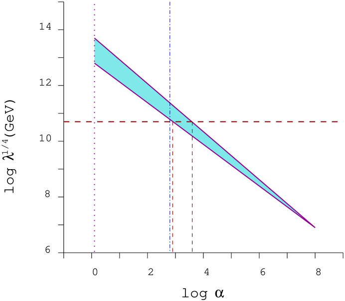
Figure 5: The shaded region depicts the allowed parameter space for the string tension $\lambda^{1/4}$ which is linked to the inflationary scale as $V^{1/4}_{\rm end}=\sqrt{b}(2\lambda)^{1/4}$. The parameter space is bounded from below by the requirements of BBN and from above by the cobe bound (solid lines). The bounds meet at $\alpha\simeq 10^{8}$, which corresponds to $\lambda_{\sc min}^{1/4}\simeq 10^{7}$GeV. The lower bound on $\alpha$ is set by the GW constraint which results in $\alpha\geq 1$ (dotted line). The dashed horizontal line depicts the case where the string tension is of the order of the intermediate scale, for which $\lambda^{1/4}=5\times 10^{10}$GeV. The vertical dashed lines correspond the the $\alpha$-range for this case. The vertical dashed–dotted line corresponds to the gravitino lower bound on $\alpha$, if not diluted by the curvaton’s decay.

$$\lambda_{\sc min}^{1/4}=7.2\times 10^{6}{\rm GeV}$$ (122)

which, in view of (6), corresponds to $M_{5}\approx 10^{11}$GeV. Now, the cobe bound, as given by (108), becomes

$$z\geq 5.08+\frac{3}{2}\ln b+\ln(N_{\rm dec}+1)$$ (123)

where $N_{\rm dec}$ is again given by (87). It can be shown that the above does not change drastically over the $\alpha$-range (when increasing $\alpha$ the mild growth of the $b_{\rm min}$ is counteracted by the decrease of $N_{\rm dec}$) and corresponds to an overall bound

$$\lambda^{1/4}\leq 2.6\times 10^{13}{\rm GeV}$$ (124)

which is satisfied over all the range (121). This bound is challenged and may be saturated only for $\alpha\approx 1$, which, however, is in danger to violate the GW constraint (and will certainly violate the gravitino constraint (66) if it is applicable). Thus, we see that without the curvaton hypothesis one can hardly secure any parameter space for successful quintessential inflation. Moreover, note that, in the context of the curvaton hypothesis, the GW and the gravitino constraints are somewhat relaxed by the entropy production due to the curvaton decay.

It can be checked that within the above parameter space a number of other constraints that apply to the system are well satisfied. In particular, one does not violate the prompt reheating constraint $\rho_{\rm reh}\leq V_{\rm end}$. Also there is an absolute upper bound on $\lambda$ coming from $\lambda^{1/4}\leq M_{5}$, which, in view of (6) is recast as

$$\lambda^{1/4}\leq\frac{8\pi}{\sqrt{6}}\,m_{P}\approx 2\,M_{P}$$ (125)

which is obviously satisfied. Another relevant bound is $V(\phi_{\rm in})<M_{5}^{4}$. Using (115) and (113) we see that this bound corresponds to

$$N_{\rm tot}<\frac{M_{5}^{4}}{2b^{2}\lambda}-1\equiv N_{\rm max}$$ (126)

Using (6) and (103) it can be shown that $N_{H}\ll N_{\rm max}$, throughout all the above parameter space and, therefore, the horizon problem is solved without problems.

As far as the spectral index is concerned it can be shown that the observational requirement (44) is not challenged in both conventional inflation and, of course, in the context of the curvaton hypothesis. Indeed, in conventional inflation we have $n_{s}-1=-\frac{4}{N+1}$, which means that (44) sets the bound $N_{\rm dec}\geq 39$. Using (87) this bound translates into $\alpha\leq 10^{12}$, which is true for all the parameter space of interest (c.f. (120)). Similarly, for the curvaton case and ignoring $\eta_{\sigma\sigma}$ we obtain the bound $\alpha\leq 10^{21}$, which is well beyond challenge. Thus, we see that, in the case of brane quintessential inflation the benefits of the curvaton hypothesis are related more to the possible reduction of the inflationary scale (allowed from the cobe bound) than to the $\eta$-problem itself. This is because steep-inflation does help reducing $|\eta|$ as long as the inflationary scale can be lowered to counteract the effect of overdamping which reduces the duration of kination. By relaxing the cobe constraint into an upper bound, the curvaton hypothesis enables us to do just that.

Finally, it should be stressed that $M$ can be anything as long as $M\leq M_{5}$, which results into the constraint:

$$A\geq\left(\frac{\sqrt{6}}{8\pi}\right)^{4/3}b^{2}\left(\frac{\lambda^{1/4}}{m_{P}}\right)^{4/3}$$ (127)

8.2.3 Example

Let us consider again the intermediate scale, $\lambda^{1/4}=5\times 10^{10}$GeV. In this case (6) gives $M_{5}=4\times 10^{13}$GeV. Then, from (121) we find the following range for $\alpha$:

$$0.8\times 10^{3}c^{-1/4}\leq\alpha\leq 3.5\times 10^{3}c^{-1/4}$$ (128)

which, again is above the gravitino bound (66). Let us choose $\alpha=2\times 10^{3}c^{-1/4}$. Then, using (116), we obtain

$$b=4.54$$ (129)

Using this and taking $c\approx 2$ we find:

$$T_{\rm reh}=\frac{\alpha b^{2}}{\sqrt{6\pi}}\frac{\sqrt{\lambda}}{m_{P}} \Rightarrow T_{\rm reh}=8\times 10^{6}{\rm GeV}$$ (130)

$$T_{*}=\frac{2\alpha^{3}b^{5}}{(12\pi)^{2}}\sqrt{\frac{2g_{\rm reh}}{5}}\left(\frac{g_{\rm reh}}{g_{*}}\right)^{1/4}\frac{\lambda}{m_{P}^{3}} \Rightarrow T_{*}=110\;{\rm MeV}$$ (131)

which are, again, overestimated by an order of magnitude, but still satisfy all the constraints, such as the gravitino bound and the BBN constraint. Also, note that $T_{\rm reh}$ is well below the so–called normalcy temperature $T_{c}\simeq\lambda^{1/4}$ [48], above which Kaluza-Klein excitations on the brane may radiate energy into the bulk and possibly reinstate the dark radiation term in (7).

Now, the $A$-bound (127) reeds

$$A\geq 5.2\times 10^{-11}$$ (132)

which, when saturated, results in $M=M_{5}$. Using (32) we find $\phi_{F}=\phi_{\rm end}+9.20\;M_{P}$, which, in view of (112) and (132) gives $\phi_{F}\leq 10.21\;M_{P}$. A preferred value of $\phi_{F}$ may be achieved by adjusting $A$, or, equivalently $M$. For example, for $M=1$ TeV we have $A=1.3\times 10^{32}$ and $\phi_{F}\simeq 5.92\;M_{P}$.

9 Conclusions

We have investigated the $\eta$-problem of quintessential inflation model-building. In the context of a potential with an exponential quintessential tail we have shown that brane cosmology inhibits the period of kination due to the extra friction on the roll-down of the scalar field. This counteracts the beneficial effects of steep inflation towards overcoming the $\eta$-problem. Hence, we pursued a different approach and considered quintessential inflation in the context of the curvaton hypothesis. We showed that the latter substantially ameliorates the $\eta$-problem in both the cases of conventional and brane cosmology. To demonstrate this we have studied a toy model of what we called modular quintessential inflation in the case of conventional cosmology and the pure exponential potential in the case of brane-cosmology. In both cases we have shown that the available parameter space for the inflationary scale is not large and it is strongly correlated with the reheating efficiency $\alpha$. Indeed, for a given $V_{\rm end}$, we have shown that there is only a small window for $\alpha$, where successful quintessential inflation is possible. This may seem like a fine-tuning problem. However, it simply reflects the necessary tuning for successful coincidence. The required values for $\alpha$ are not unreasonable and we should point out that there is nothing special about the present time. Any value of $\alpha$ would cause some brief acceleration period in the late Universe. We just happen to live in this period. These tuning considerations are even more relaxed if one considers the possibility of multiple unfreezings and refreezings of the scalar field, as discussed at the end of Sec. 5.2.

In this paper we have considered the intriguing possibility that the scalar field of quintessential inflation (called the ‘cosmon’ by some authors) is a modulus field, possibly associated with the volume of the extra dimensions, such as the geometrical $T$-moduli of weakly coupled heterotic string theory. The modulus is taken to roll down and away from the origin, where it could have been placed by temperature corrections to its potential during a period of thermalization preexisting inflation, if the origin is a point of enhanced symmetry. In this scenario the inflationary expansion begins with a period of thermal inflation followed by fast-roll inflation, as described in [25] for modular thermal inflation. In contrast to [25] though, we have supposed that the Kähler corrections introduce an exponential slope to the potential over distances comparable to $m_{P}$ in field space. Thus, the VEV of the modulus is displaced at infinity, while the modulus is stabilized dynamically by being frozen during the later history of the Universe at a non-zero potential density, causing the present accelerated expansion. This way it may be natural to avoid the excessive supergravity corrections that would otherwise increase the present mass of quintessence to unacceptable values. However, it remains to be seen whether this scenario is possible in the context of a realistic string theory.

Turning to brane cosmology we have focused in the much investigated pure exponential potential, which may also be motivated by string theory considerations. In this case there is no preferred starting point for the roll down of the field as long as the inflationary energy scale is kept below the fundamental scale of the theory. We have seen that the parameter space for successful quintessential inflation is somewhat reduced by the negative overdamping effect of brane-cosmology on kination.

Finally, we have studied the effects of gravitational wave generation on quintessential inflationary model-building. We have shown that gravitational waves will not destabilize BBN if the reheating efficiency is $\alpha>1$, which may require some tiny, but non-zero coupling of the inflaton with other fields. In the context of the curvaton hypothesis, however, the gravitational wave constraint is ameliorated by the dilution effect of the entropy production due to the curvaton’s decay. This may lower the bound on $\alpha$ below $\alpha\sim 0.1$, which will render gravitational reheating (and a truly sterile inflaton) acceptable. However, a larger $\alpha$ may be necessary in order to avoid gravitino overproduction: $\alpha\mbox{\raisebox{-3.87495pt}{~{}$\stackrel{{\scriptstyle\mbox{$>$}}}{{\sim}}$~{}}}10^{2}$. Note, here, that tiny couplings between the inflaton and the SM fields may have beneficiary side effects, such as baryogenesis [40].

All in all we have shown that the liberating effect of the curvaton hypothesis enables quintessential inflation to overcome its $\eta$-problem and enlarges the parameter space for successful model-building. Appealing candidates for the quintessential inflaton (or cosmon) may be string–moduli fields.

Acknowledgments

I would like to thank D.H. Lyth and J.E. Lidsey for discussions. This work was supported by the E.U. network program: HPRN-CT00-00152.

References

- [1] S. Perlmutter et al. [Supernova Cosmology Project Collaboration], Astrophys. J. 517, 565 (1999) [arXiv:astro-ph/9812133]; A. G. Riess et al. [Supernova Search Team Collaboration], Astron. J. 116, 1009 (1998) [arXiv:astro-ph/9805201]; B. P. Schmidt et al., Astrophys. J. 507, 46 (1998) [arXiv:astro-ph/9805200]; P. M. Garnavich et al., Astrophys. J. 493, L53 (1998) [arXiv:astro-ph/9710123].
- [2] R. G. Carlberg et al., arXiv:astro-ph/9703107; N. A. Bahcall, J. P. Ostriker, S. Perlmutter and P. J. Steinhardt, Science 284, 1481 (1999) [arXiv:astro-ph/9906463]; M. Tegmark, Astrophys. J. 514, L69 (1999) [arXiv:astro-ph/9809201]; A. H. Jaffe et al. [Boomerang Collaboration], Phys. Rev. Lett. 86, 3475 (2001) [arXiv:astro-ph/0007333].
- [3] A. Vikhlinin et al., arXiv:astro-ph/0212075.
- [4] E. W. Kolb and M. S. Turner, The Early Universe, Addison-Wesley Publishing Company, Reading 1993.
- [5] A. R. Liddle and D. H. Lyth, Cosmological Inflation and Large Scale Structure, Cambridge University Press, Cambridge 2000.
- [6] S. Weinberg, Rev. Mod. Phys. 61, 1 (1989).
- [7] L. M. Wang, R. R. Caldwell, J. P. Ostriker and P. J. Steinhardt, Astrophys. J. 530, 17 (2000) [arXiv:astro-ph/9901388]; I. Zlatev, L. M. Wang and P. J. Steinhardt, Phys. Rev. Lett. 82, 896 (1999) [arXiv:astro-ph/9807002];
- [8] G. Huey, L. M. Wang, R. Dave, R. R. Caldwell and P. J. Steinhardt, Phys. Rev. D 59, 063005 (1999) [arXiv:astro-ph/9804285]; R. R. Caldwell, R. Dave and P. J. Steinhardt, Phys. Rev. Lett. 80, 1582 (1998) [arXiv:astro-ph/9708069].
- [9] C. F. Kolda and D. H. Lyth, Phys. Lett. B 458, 197 (1999) [arXiv:hep-ph/9811375].
- [10] P. J. Peebles and A. Vilenkin, Phys. Rev. D 59, 063505 (1999) [arXiv:astro-ph/9810509].
- [11] S. C. Ng, N. J. Nunes and F. Rosati, Phys. Rev. D 64, 083510 (2001) [arXiv:astro-ph/0107321].
- [12] Kinney and Riotto 1999; Peloso and Rosati 1999 W. H. Kinney and A. Riotto, Astropart. Phys. 10, 387 (1999) [arXiv:hep-ph/9704388]; M. Peloso and F. Rosati, JHEP 9912, 026 (1999) [arXiv:hep-ph/9908271].
- [13] K. Dimopoulos and J. W. Valle, Astropart. Phys. 18, 287 (2002) [arXiv:astro-ph/0111417]; K. Dimopoulos, Nucl. Phys. Proc. Suppl. 95, 70 (2001) [arXiv:astro-ph/0012298].
- [14] K. Dimopoulos, arXiv:astro-ph/0210374.
- [15] G. Huey and J. E. Lidsey, Phys. Lett. B 514, 217 (2001) [arXiv:astro-ph/0104006].
- [16] A. S. Majumdar, Phys. Rev. D 64, 083503 (2001) [arXiv:astro-ph/0105518]; N. J. Nunes and E. J. Copeland, Phys. Rev. D 66, 043524 (2002) [arXiv:astro-ph/0204115].
- [17] G. J. Mathews, K. Ichiki, T. Kajino, M. Orito and M. Yahiro, arXiv:astro-ph/0202144.
- [18] G. N. Felder, L. Kofman and A. D. Linde, Phys. Rev. D 60, 103505 (1999) [arXiv:hep-ph/9903350].
- [19] Ford 1986; Grishchuk and Sidorov 1990; Kuzmin and Tkachev 1999 L. H. Ford, Phys. Rev. D 35, 2955 (1987); L. P. Grishchuk and Y. V. Sidorov, Phys. Rev. D 42, 3413 (1990); V. Kuzmin and I. Tkachev, Phys. Rev. D 59, 123006 (1999) [arXiv:hep-ph/9809547].
- [20] M. Joyce and T. Prokopec, Phys. Rev. D 57, 6022 (1998) [arXiv:hep-ph/9709320].
- [21] B. Spokoiny, Phys. Lett. B 315, 40 (1993) [arXiv:gr-qc/9306008].
- [22] L. Amendola, Phys. Rev. D 62, 043511 (2000) [arXiv:astro-ph/9908023].
- [23] E. J. Copeland, A. R. Liddle and J. E. Lidsey, Phys. Rev. D 64, 023509 (2001) [arXiv:astro-ph/0006421].
- [24] D. H. Lyth and D. Wands, Phys. Lett. B 524, 5 (2002) [arXiv:hep-ph/0110002]; D. H. Lyth, C. Ungarelli and D. Wands, arXiv:astro-ph/0208055.
- [25] K. Dimopoulos and D. H. Lyth, arXiv:hep-ph/0209180.
- [26] J. M. Cline, C. Grojean and G. Servant, Phys. Rev. Lett. 83, 4245 (1999) [arXiv:hep-ph/9906523].
- [27] P. Binetruy, C. Deffayet, U. Ellwanger and D. Langlois, Phys. Lett. B 477, 285 (2000) [arXiv:hep-th/9910219]; P. Binetruy, C. Deffayet and D. Langlois, Nucl. Phys. B 565, 269 (2000) [arXiv:hep-th/9905012]; T. Shiromizu, K. i. Maeda and M. Sasaki, Phys. Rev. D 62, 024012 (2000) [arXiv:gr-qc/9910076].
- [28] A. H. Campos, H. C. Reis and R. Rosenfeld, arXiv:hep-ph/0210152.
- [29] G. N. Felder, L. Kofman and A. D. Linde, Phys. Rev. D 59, 123523 (1999) [arXiv:hep-ph/9812289].
- [30] S. Hellerman, N. Kaloper and L. Susskind, JHEP 0106, 003 (2001) [arXiv:hep-th/0104180]; W. Fischler, A. Kashani-Poor, R. McNees and S. Paban, JHEP 0107, 003 (2001) [arXiv:hep-th/0104181]; E. Witten, arXiv:hep-th/0106109.
- [31] E. J. Copeland, A. R. Liddle and D. Wands, Phys. Rev. D 57, 4686 (1998) [arXiv:gr-qc/9711068].
- [32] J. M. Cline, JHEP 0108, 035 (2001) [arXiv:hep-ph/0105251]; C. F. Kolda and W. Lahneman, arXiv:hep-ph/0105300.
- [33] P. G. Ferreira and M. Joyce, Phys. Rev. D 58, 023503 (1998) [arXiv:astro-ph/9711102].
- [34] M. Giovannini, Class. Quant. Grav. 16, 2905 (1999) [arXiv:hep-ph/9903263]; M. Giovannini, Phys. Rev. D 60, 123511 (1999) [arXiv:astro-ph/9903004].
- [35] V. Sahni, M. Sami and T. Souradeep, Phys. Rev. D 65, 023518 (2002) [arXiv:gr-qc/0105121].
- [36] D. Langlois, R. Maartens and D. Wands, Phys. Lett. B 489, 259 (2000) [arXiv:hep-th/0006007].
- [37] R. Kallosh, L. Kofman, A. D. Linde and A. Van Proeyen, Phys. Rev. D 61, 103503 (2000) [arXiv:hep-th/9907124].
- [38] P. Salati, arXiv:astro-ph/0207396.
- [39] T. Matos, F. S. Guzman, L. A. Urena-Lopez and D. Nunez, arXiv:astro-ph/0102419.
- [40] A. De Felice, S. Nasri and M. Trodden, arXiv:hep-ph/0207211; M. Yamaguchi, arXiv:hep-ph/0211163.
- [41] C. M. Hull and P. K. Townsend, Nucl. Phys. B 451, 525 (1995) [arXiv:hep-th/9505073]; E. Witten, Nucl. Phys. B 443, 85 (1995) [arXiv:hep-th/9503124].
- [42] T. Barreiro, B. de Carlos and N. J. Nunes, Phys. Lett. B 497, 136 (2001) [arXiv:hep-ph/0010102]; P. Brax and J. Martin, Phys. Rev. D 61, 103502 (2000) [arXiv:astro-ph/9912046]; E. J. Copeland, N. J. Nunes and F. Rosati, Phys. Rev. D 62, 123503 (2000) [arXiv:hep-ph/0005222].
- [43] T. Damour and A. Vilenkin, Phys. Rev. D 53, 2981 (1996) [arXiv:hep-th/9503149].
- [44] A. R. Frey and A. Mazumdar, arXiv:hep-th/0210254.
- [45] A. Linde, JHEP 0111, 052 (2001) [arXiv:hep-th/0110195].
- [46] R. Maartens, D. Wands, B. A. Bassett and I. Heard, Phys. Rev. D 62, 041301 (2000) [arXiv:hep-ph/9912464].
- [47] J. P. Derendinger, L. E. Ibanez and H. P. Nilles, Phys. Lett. B 155, 65 (1985); M. Dine, R. Rohm, N. Seiberg and E. Witten, Phys. Lett. B 156, 55 (1985).
- [48] R. Allahverdi, A. Mazumdar and A. Perez-Lorenzana, Phys. Lett. B 516, 431 (2001) [arXiv:hep-ph/0105125].