Dark energy effects on the Lyman-$\alpha$ forest

Abstract

In quintessence models, the dark energy content of the universe is described by a slowly rolling scalar field whose pressure and energy density obey an equation of state of the form $p=w\rho$; $w$ is in general a function of time such that $w<-1/3$, in order to drive the observed acceleration of the Universe today. The cosmological constant model ($\Lambda$CDM) corresponds to the limiting case $w=-1$. In this paper, we explore the prospects of using the Lyman-$\alpha$ forest to constrain $w$, using semi-analytical techniques to model the intergalactic medium (IGM). A different value of $w$ changes both the growth factor and the Hubble parameter as a function of time. The resulting change in the optical depth distribution affects the optical depth power spectrum, the number of regions of high transmission per unit redshift and the cross-correlation coefficient of spectra of quasar pairs. These can be detected in current data, provided we have independent estimates of the thermal state of the IGM, its ionization parameter and the baryon density.

1 Introduction

Observed cosmic microwave background anisotropies convincingly demonstrate that the universe is spatially flat (de Bernardis et al. 2002; Netterfield et al. 2002; Pryke et al. 2002). The luminosity-distance relation, as determined from high redshift type Ia Supernovae (Garnavich et al. 1998; Riess et al. 1998; Perlmutter et al. 1999), requires a spatially flat universe to be currently dominated by some type of dark energy, which is nearly homogeneous and has negative pressure, such as for example a cosmological constant. Several independent lines of argument also favour a low-density, vacuum-energy dominated universe, for example the abundance of clusters (Bahcall et al. 2003) and their X-ray properties (Allen et al. 2002), the clustering of galaxies (Efstathiou et al. 2002; Verde et al. 2002), estimates of the age of the universe and the current value of the Hubble parameter.

The energy density associated with the cosmological constant may actually decay in time. Such quintessence models (e.g. Caldwell et al. 1998; henceforth QCDM models) have an equation of state $p=w\,\rho$, with $w<-1/3$, where $w=-1$ corresponds to the more familiar cosmological constant model. Recently, a number of observational tests have been proposed to measure $w$ and its redshift dependence (Kujat et al. 2001; Wang & Garnavich 2001; Matsubara & Szalay 2002; Gerke & Efstathiou 2002).

In this Letter we focus on the prospects of using the Lyman-$\alpha$ forest to constrain $w$. The Lyman-$\alpha$ forest region in quasar (QSO) spectra contains hundreds of hydrogen Lyman-$\alpha$ absorption lines (see Rauch 1998 for a review), most of which are produced by small density fluctuations in the intervening intergalactic medium (Cen et al. 1994; Bi & Davidsen 1997, hereafter BD97). Since these structures are still reasonably linear, they are good probes of the underlying large-scale matter distribution, and hence are sensitive to the cosmological model. For example, Hui et al. (1999) and McDonald (2001) suggested to apply the Alcock-Paczinski test (Alcock & Paczinski 1979) to estimate the cosmological constant and Croft et al. (2002) constrained the dark matter power spectrum on large scales. The Lyman-$\alpha$ forest is promising in that it can be used over a larger redshift range than most other potential probes of $w$.

Here we use semi-analytical models of the Lyman-$\alpha$ forest, which have been shown to be successful in reproducing reasonably well most of its observed properties, such as the column density distribution function, the line-widths distribution and the number of lines per unit redshift (BD97; Viel et al. 2002a, 2002b; Roy Choudury et al. 2001). Hydrodynamical simulations are required for more accurate predictions on smaller scales (e.g. Theuns et al. 1998, 2002; Davé et al. 1999; Bryan et al. 1999). We examine several statistics of the flux spectrum, such as the probability distribution function of the optical depth, the optical depth power spectrum, the number of underdense regions per unit redshift and the cross-correlation coefficient of spectra of quasar pairs. The first two statistics are not directly observable but they can be recovered from the flux distribution by looking at higher order lines through pixel optical depths techniques (Sect. 3). Section 2 briefly reviews the properties of quintessence models and describes our simulation techniques. Section 3 contains our results and a brief discussion.

2 Simulations of Lyman-$\alpha$ spectra in quintessence models

The quintessence parameter $w$ influences the shape of the linear matter power spectrum $P(k,z)\propto k^{n}\,{\cal T}^{2}(k,z)\,D^{2}(z)$, the linear growth factor of density perturbations $D(z)$ and the Hubble parameter $H(z)$. Here $k$ is the wavenumber, ${\cal T}$ the transfer function and $n$ the spectral index. Useful expressions for the growth factor of density perturbations and of linear peculiar velocities can be found in Lahav et al. (1991), for $\Lambda$CDM, and in Wang & Steinhardt (1998), for QCDM. The Hubble parameter at redshift $z$ is $H(z)=H_{0}\left[\Omega_{m}(1+z)^{3}+\Omega_{k}(1+z)^{2}+\Omega_{DE}(1+z)^{3+3w}\right]^{1/2}$, with $H_{0}=100\,h$ km s^-1 the present-day Hubble parameter and $\Omega_{k}=1-\Omega_{m}-\Omega_{DE}$. $\Omega_{DE}$ represents the energy density of the cosmological constant ($\Omega_{\Lambda}$) or the quintessence ($\Omega_{Q}$), in units of the critical density.

In Figure 1 we plot ${\cal T}(k,z)$, $D(z)$ and the Hubble parameter $H(z)$, for several values of $w$, here assumed to be constant in time, for simplicity, using the fits of Ma et al. (1999). If we compare the transfer function of QCDM and $\Lambda$CDM at $z=2$ one can see that there are differences only on very large scales, $k\mbox{$\;\buildrel<\over{\sim}\;$}0.01\,h$  Mpc^-1. The Hubble parameter in QCDM models with $w=-0.8$, $-0.6$ and $-0.4$ differs by 6, 14 and 25 per cent at redshifts $z\sim 0.75$, $z\sim 1$ and $z\sim 1.2$ from those of the $\Lambda$CDM model (panel b). For those values of $w$, the growth factors $D(z)$ (panel c) at $z\sim 2$ are larger than for the $\Lambda$CDM model by 5, 15 and 30 per cent respectively.

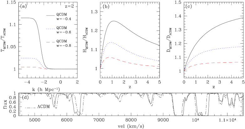
Figure 1: Panel a): ratio of transfer functions ${\cal T}_{QCDM}/{\cal T}_{\Lambda CDM}$ at z=2. Panel b): ratio of Hubble parameters $H_{QCDM}/H_{\Lambda CDM}$ as a function of redshift. Panel c): ratio of growth factors $D_{QCDM}/D_{\Lambda CDM}$ as a function of redshift. The three curves shown are for three quintessence models with $w=-0.4$ (continuous line), $w=-0.6$ (dotted line) and $w=-0.8$ (dashed line). Panel d): example of simulated spectra, it is shown $\Lambda$CDM spectra (dot-dashed line) and the QCDM with $w=-0.4$ (continuous line).

The semi-analytical model we use to generate Lyman-$\alpha$ forest spectra is based on the approximations introduced by Bi and collaborators (BD97; see Viel et al. (2002a) for more details). The basic assumption is that the low-column density Ly$\alpha$ forest is produced by smooth fluctuations in the intergalactic medium (IGM), which arise as a result of gravitational growth of perturbations (e.g. Schaye 2001). Briefly, we start by generating correlated Gaussian random fields to represent the linear density and peculiar velocity dark matter fields along a sight-line, for a given linear matter power spectrum. The linear density perturbations in the IGM $\delta_{0}^{\rm IGM}({\bf x},z)$ are related to those in the underlying dark matter by a convolution, $\delta_{0}^{\rm IGM}({\bf k},z)=W_{\rm IGM}(k,z)\delta_{0}^{\rm DM}({\bf k},z)$. For the smoothing kernel $W$ we use the Gaussian filter $W_{IGM}=\exp(-k/k_{f})^{2}$ (Gnedin et al. 2002), which is a good approximation to model the effects of gas pressure in the linear regime. The smoothing scale $k_{f}$ is related to the Jeans length in a way which depends on the thermal history of the IGM (Gnedin & Hui 1998; Matarrese & Mohayaee 2002).

To account for the fact that the IGM which produces most of the Lyman-$\alpha$ forest is actually mildly non-linear, we follow BD97 and adopt a simple lognormal model (Coles & Jones 1991) for the IGM local density. This is a strong assumption but we think that at these redshift and for the large scale properties investigated here the log-normal model can be a good approximation to the more accurate hydro-dynamical simulations. We assume the gas to be in photoionization equilibrium with an imposed uniform UV-background, which we scale so that the mock spectra have the same effective optical depth $\tau_{\rm eff}$ as observed (see Kim et al. 2002 and Bernardi et al. 2002, for recent determinations of $\tau_{eff}(z)$). We use the values of Schaye et al. (2000) for the normalization $T_{0}$ and slope $\gamma$ of the temperature-density relation, $T=T_{0}(\rho/\langle\rho\rangle)^{\gamma-1}$, in the IGM. Finally, we artificially broaden the spectra to a resolution of FWHM = 6.6 km s^-1 to mimic high quality VLT/UVES or Keck/HIRES spectra, and add Gaussian noise with signal to noise of 50 (see e.g. Theuns et al. 2000 for more details). Spectra generated with this procedure have been shown to produce flux probability and line-width distribution functions in reasonable agreement with observations (BD97).

We will compare the Lyman-$\alpha$ forest in a $\Lambda$CDM cosmological model with three different QCDM models, with $w=-0.4,-0.6,-0.8$, respectively. For all of these models, we assume that the cosmological parameters are $\sigma_{8}=0.7,\Omega_{m}=0.3,h=0.67,\Omega_{b}\,h^{2}=0.020,\,\Omega_{DE}=0.7$. We simulate 10 different randomly generated spectra, with the same set of random phases for each spectrum, in the redshift range $1.8<z<2.2$ for each model, assuming $\tau_{eff}=0.15$ (Kim et al. 2002), $\gamma=1.3$ and $T_{0}=10^{4.1}$ K. The filtering scale is $k_{f}\sim 1.7\,k_{J}$ (with $k_{J}$ the Jeans wave-number), which is a reasonable estimate if HI reionization takes place at $z\sim 7$ (Gnedin & Hui 1998). The spectra are approximately $40,000$ km s^-1 long. In addition, we simulate spectra of QSO pairs with a given angular separation in the range 10–90 arcsec, using the procedure described in Viel et al. (2002a). The cross-correlation coefficient spectra of pairs is estimated using the definition of Viel et al. (2002a) from a set of 8 pairs for each separation. In panel d) of Figure 1 we show, for a qualitative comparison, a chunk of two simulated spectra for the $\Lambda$CDM and QCDM, with $w=-0.4$, model. We have decided to focus our analysis around $z\sim 2$ in view of a comparison with observations which will be made in a future work.

3 Results

In this section we will study the effects of dark energy on the simulated spectra. The differences between the QCDM and $\Lambda$CDM model, which could be tested through Lyman-$\alpha$ absorptions, are the following: the linear dark matter power spectrum $P(k,z)$; the evolution of the cosmological parameters and in particular of the Hubble parameter $H(z)$; the growth factors $D(z)$ of the linear density perturbations.

The simulated Lyman-$\alpha$ flux power spectrum agrees reasonably well with the linear dark matter power spectrum at large scales, while on smaller scales non-linear effects, thermal broadening and noise can produce differences. This is roughly true even if we do not correct for redshift-space distortions and compare directly the flux power spectrum of simulated absorption spectra and the linear dark matter power spectrum. From Figure 1 (panel a) we can see that the QCDM transfer function differs from the $\Lambda$CDM one only on scales larger than 100 comoving Mpc. Such scales are comparable to the extent of the Lyman-$\alpha$ forest region in a QSO spectrum, and hence this signature of $w\neq-1$ would be difficult to detect since it would require a large number of spectra to estimate the power on these scales. More importantly, in high resolution spectra every attempt to recover the power spectrum on scales larger than 10 comoving Mpc is challenging due to the continuum fitting uncertainties (Croft et al. 1999).

A second difference between QCDM and $\Lambda$CDM is the different evolution of the cosmological parameters, such as $H(z)$. We have explored the effect of a different Hubble parameter and different growth factors values at redshift $z=2$ on the simulated Lyman-$\alpha$ optical depth, by fixing the remaining parameters. The effect is clear: a larger Hubble parameter produces in general a broader optical depth distribution with the peak shifted to lower values. In fact, with a higher value of the Hubble parameter, the same real-space absorber intersected by the sight-line will affect a larger region of the redshift-space spectrum.

In the same way, we explore the effect of different growth factors. If the growth factor is increased, the (non-linear) log-normal mapping acts in such a way that typically the low-density regions become less dense and the high-density regions more dense. Thus, with a larger growth factor, as the one predicted for QCDM models compared to $\Lambda$CDM ones (Figure 1, panel c), the simulated optical depth shifts to smaller values and its probability distribution function (pdf) becomes broader. This effect can be seen also in the simulated flux in panel d) of Figure 1, for example at $\sim 6000$ km s^-1 this is particularly evident.

Our first conclusion is that a larger growth factor produces the same effect of a higher value of the Hubble parameter: a shift of the simulated Lyman-$\alpha$ optical depth to smaller values and a broader distribution, if the other parameters remain fixed.

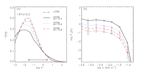
Figure 2: Panel a): probability distribution function of the optical depth (panel a) for QCDM model with $w=-0.4$ (continuous line), $w=-0.6$ (dotted line), $w=-0.8$ (dashed line) and $\Lambda$CDM model (dot-dashed line). The interval in which the optical depth can be recovered directly from the flux is represented by the double arrow (a larger range can be used with pixel optical depth technique, see text). Panel b): power spectrum of the optical depth; error bars represent the error of the mean.

To see these effects combined together, we plot in panel a) of Figure 2 the probability distribution function of the simulated optical depth for $\Lambda$CDM (dot-dashed line), QCDM with $w=-0.4$ (continuous line), $w=-0.6$ (dotted line) and $w=-0.8$ (dashed line). We choose to plot the probability distribution function also for $\tau$ values smaller than those which can actually be recovered by standard techniques to better appreciate the differences between cosmological models. We can see that the simulated optical depth pdf results in different distributions for the four cosmological models. Since the flux is the observed quantity, the inferred optical depth can be trusted only in the range $-1.6\raise-2.0pt\hbox{\hbox to0.0pt{\hbox{$\sim$}\hss}\raise 5.0pt\hbox{$<$}\ }\log(\tau)\raise-2.0pt\hbox{\hbox to0.0pt{\hbox{$\sim$}\hss}\raise 5.0pt\hbox{$<$}\ }0.5$ (corresponding to fluxes in the range 0.04-0.97). With a more sophisticated analysis, based on pixel optical depth techniques, this range can be considerably extended (Aguirre et al. 2002 and references therein). In panel b) of Figure 2 we plot the optical depth power spectrum for the QCDM and the $\Lambda$CDM model, with Poissonian error bars. We can see that on scales $\log k\,(\rm{km\,s}^{-1})<-1.5$ the four cosmological models are distinguishable: while the shape is very similar, the normalization is different even if we choose the same value for $\tau_{eff}$. This is the effect of different amounts of non linearity in the four cosmological models, which influences the normalization of the curves.

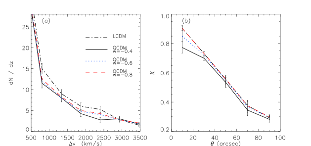
Figure 3: Number of underdense regions per unit redshift as a function of void size in km s^-1 (panel a) for the three QCDM models with $w=-0.4$ (continuous line), $w=-0.6$ (dotted line), $w=-0.8$ (dashed line) and $\Lambda$CDM model (dot-dashed line). The simulated sample consists of 10 spectra, spanning the redshift range $1.8<z<2.2$ for each cosmological model. Cross-correlation coefficient, $\chi$, as a function of QSO pair separation in arcsec (panel b). The simulated sample consists of 8 QSO pairs for each separation shown. Poissonian error bars in panel a), shown only for two different models for clarity. In panel b) the error bars are the errors of the mean value.

In Figure 3 we plot two more observational quantities: the number of underdense regions per unit redshift (panel a) and the cross-correlation coefficient $\chi$ estimated from the spectra of QSO pairs at different separations (panel b). The definition of underdense region adopted here is the following: if we are searching for an underdense region of size $\Delta v$, we preliminarily smooth the simulated spectra on this scale (top-hat smoothing) and then we define as an underdensity a region for which the flux is larger than the mean flux at that redshift, estimated through $\tau_{eff}$. One can see that the predicted number of underdense regions per unit redshift is different for the four cosmological models. The number of underdense regions of intermediate sizes, between 700 km s^-1 and 2700 km s^-1, which correspond to sizes in the range 10-40 comoving Mpc in a $\Lambda$CDM universe, is larger in the $\Lambda$CDM model than in the QCDM ones. This is due to the combined effects of a different Hubble parameters and a different growth factor for density perturbations, as we saw in panel a) of Figure 2, which produce more rarefied underdense region and denser high density regions in QCDM models than in $\Lambda$CDM models. In particular, we have found that the number of underdense regions of size 2500 km s^-1 for $\Lambda$CDM can be a factor of 2 and 1.5 larger than in QCDM model with $w=-0.4$ and $w=-0.8$ at $z=2$, respectively.

The cross-correlation coefficient $\chi$ is plotted in panel b) of Figure 3, this number quantifies the amount of ‘coherence’ in the transverse direction between spectra of QSO pairs. The information contained in the transverse direction could be powerful and has already been analysed in the past (Miralda-Escudé et al. 1996; Viel et al. 2002a). This test is in a sense similar to the more sophisticated Alcock-Paczinski test (Hui et al. 1999; McDonald & Miralda-Escudé 1999; McDonald 2001) and aims at discriminating between different cosmological models. Here, we have simulated 8 QSO pairs at $z\sim 2$ for five separations (10, 30, 50, 70 and 90 arcsec) and computed the mean value and the error of the mean for this coefficient at each separation. The four models are very similar and the error bars overlap. Only at angular scales $\raise-2.0pt\hbox{\hbox to0.0pt{\hbox{$\sim$}\hss}\raise 5.0pt\hbox{$<$}\ }20$ arcsec there are some differences between the models. However, the number of pairs considered here is marginally sufficient to discriminate between a $\Lambda$CDM model and a QCDM with $w=-0.4$. We have estimated that 25 pairs with these small separations are needed to distinguish between the $\Lambda$CDM model and a QCDM with $w=-0.6$ at a 3$\sigma$ level.

Dark energy in the form of quintessence in the Lyman-$\alpha$ forest seems to be not easily distinguishable from a cosmological constant. Even if the thermal state of the IGM is completely known, the uncertainties on the values of the baryon fraction (Burles et al. 2001) and especially on the ionization parameter (Scott et al. 2000), are so large that it would be difficult to recover the evolution of $H(z)$. We have found that a QCDM model with $w=-0.4$ requires an ionization parameter a factor of 3 lower than in a $\Lambda$CDM model (while for $w=-0.8$ it is a factor of 1.25 lower), in order to match observed $\tau_{eff}$. Uncertainties on the value of $\tau_{eff}$ are of the order of 40%, but in the near future, with larger data set available, this uncertainty will become significantly smaller. In principle, an accurate determination of $\tau_{eff}$, with a precision of $10-20\%$ could already be used to discriminate between QCDM with $w=-0.4$ and $\Lambda$CDM models, since the present uncertainties on the ionization parameter are of the order of 50%. Statistics based on the optical depth like the pdf or the power spectrum, instead of the flux, can be much more useful in discriminating between different cosmological models. This is due to the fact that the optical depth is very sensitive to the amount of non-linearity introduced in the different cosmological models. However, in order to do that, it will be necessary to use pixel optical depth techniques, using higher order Lyman lines, to get reliable estimates of the optical depths both in saturated and in high transmissivity regions.

In summary, we have presented a preliminary analysis of simulated spectra in QCDM models and in a $\Lambda$CDM model based on semi-analytical models. The main differences can be found in the different evolution of $H(z)$ and of the linear growth factor of density perturbations $D(z)$. Both these effects act in a similar way. If we fix the remaining parameters and compare the probability distribution function of Lyman-$\alpha$ optical depth between QCDM and $\Lambda$CDM we have found that the distribution in the QCDM model is broader than in the $\Lambda$CDM case. This means that in general high transmission regions are more rarefied and high density regions are denser in QCDM than in a $\Lambda$CDM universe. The optical depth power spectrum is different on intermediate and large scales, even if the normalization $\tau_{eff}$ is the same, because of the different amounts of non linearity predicted for the models. Detecting the underdense regions could be promising. In fact, we have found that the number of intermediate size underdense regions, with sizes of the order of 10 comoving Mpc, is larger in a $\Lambda$CDM model than in QCDM ones. Another statistics we have proposed concerns the the cross-correlation coefficient between the spectra of QSO pairs. However, in this case, the differences can be appreciated only for separations smaller than 20 arcsec and the number of pairs should be larger than 20 to distinguish between QCDM and $\Lambda$CDM cosmological models at a 3$\sigma$ level.

References

- [] Aguirre A., Schaye J., Theuns T., 2002, ApJ, 576, 1
- [] Alcock C., Paczynski B, 1979, Nature, 281, 358
- [] Allen S.W. et al. 2002, preprint,astro-ph/0208394
- [] Bahcall N.A. et al. 2003, ApJ, 585
- [] Bernardi M. et al. 2002, AJ, in press
- [] Bi H.G., Davidsen A.F., 1997, ApJ, 479, 523
- [] Bryan, G. L. et al. 1999, ApJ, 517, 13
- [] Burles S. et al. 2001, ApJ, 552, 1
- [] Caldwell R.R. et al. 1998, Phys.Rev.Lett., 80, 1582
- [] Cen R. et al. 1994, ApJ, 437, L9
- [] Coles P., Jones B., 1991, MNRAS, 248, 1
- [] Croft R.A.C. et al. 1999, ApJ, 520, 1
- [] Croft R.A.C. et al. 2002, ApJ, in press
- [] Davé R. et al. 1999, ApJ, 511, 521
- [] de Bernardis P. et al. 2002, ApJ, 564, 559
- [] Efstathiou G. et al. 2002, MNRAS, 330, L29
- [] Garnavich P.M. et al. 1998, AAS, 193, 3905
- [] Gerke B.F., Efstahiou G., 2002, MNRAS, 335, 33
- [] Gnedin N.Y., Hui L., 1998, MNRAS, 296, 44
- [] Gnedin N.Y. et al. , 2002, preprint, astro-ph/0206421
- [] Hui L., Stebbins A. Burles S., 1999, ApJ, 511, 5
- [] Kujat J. et al. 2002, ApJ, 572, 1
- [] Kim T.-S. et al. , 2002, MNRAS, 335, 555
- [] Lahav O. et al. , 1991, MNRAS, 251 128
- [] Ma C-P., Caldwell R.R., Bode P., Wang L., 1999, ApJL, 521
- [] Matarrese S., Mohayaee, R., 2002, MNRAS, 329, 37
- [] Matsubara T., Szalay A.S., 2002, astro-ph/0208087
- [] McDonald P., 2001, astro-ph/0108064
- [] McDonald P., Miralda-Escudé J., 1999, ApJ, 518, 24
- [] Miralda-Escudé J. et al. 1996, ApJ, 471, 582
- [] Netterfield C.B. et al. 2002, ApJ, 571, 604
- [] Perlmutter S. et al. 1999, ApJ, 517, 565
- [] Pryke C. et al. 2002, ApJ, 568, 46
- [] Rauch M., 1998, ARA&A, 36, 267
- [] Riess A.G. et al. 1998, AJ, 116, 1009
- [] Roy Choudhury T. et al. , 2001, MNRAS, 322, 561
- [] Schaye J., 2001, ApJ, 559, 507
- [] Schaye J. et al. , 2000, MNRAS, 318, 817
- [] Scott J. et al. 2000, ApJ, 130, 67
- [] Theuns T., Schaye J., Haehnelt M., 2000, MNRAS, 315, 600
- [] Theuns T. et al. 1998, MNRAS, 301, 478
- [] Theuns T., Viel M., Kay S., Schaye J., Carswell B., Tzanavaris P., 2002, ApJ, 578, L5
- [] Verde L., Heavens A.F., Percival W., Matarrese S. et al. , 2002, MNRAS, 335, 432
- [] Viel M., Matarrese S., Mo H.J., Haehnelt M.G., Theuns T., 2002a, MNRAS, 329, 848
- [] Viel M., Matarrese S., Mo H.J., Theuns T., Haehnelt M.G., 2002b, MNRAS, 336, 685
- [] Wang L., Steinhardt P.J., 1998, ApJ, 508, 483
- [] Wang Y., Garnavich, P.M., 2001, ApJ, 552, 445