THE EVOLUTION OF THE GLOBAL STELLAR MASS DENSITY
AT $0<z<3$

Abstract

The build–up of stellar mass in galaxies is the consequence of their past star formation and merging histories. Here we report measurements of rest–frame optical light and calculations of stellar mass at high redshift based on an infrared–selected sample of galaxies from the Hubble Deep Field North. The bright envelope of rest–frame $B$–band galaxy luminosities is similar from $0<z<3$, and the co–moving luminosity density is constant to within a factor of 3 over that redshift range. However, galaxies at higher redshifts are bluer, and stellar population modeling indicates that they had significantly lower mass–to–light ratios than those of present–day $L^{\ast}$ galaxies. This leads to a global stellar mass density, $\Omega_{\ast}(z)$, which rises with time from $z=3$ to the present. This measurement essentially traces the integral of the cosmic star formation history that has been the subject of previous investigations. 50–75% of the present–day stellar mass density had formed by $z\sim 1$, but at $z\approx 2.7$ we find only 3–14% of today’s stars were present. This increase in $\Omega_{\ast}$ with time is broadly consistent with observations of the evolving global star formation rate once dust extinction is taken into account, but is steeper at $1<z<3$ than predicted by some recent semi–analytic models of galaxy formation. The observations appear to be inconsistent with scenarios in which the bulk of stars in present–day galactic spheroids formed at $z\gg 2$.

1 Introduction

One goal of observational cosmology is to understand the history of mass assembly in galaxies. In current models of structure formation, dark matter halos build up in a hierarchical process controlled by the nature of the dark matter, the power spectrum of density fluctuations, and the parameters of the cosmological model. The assembly of the stellar content of galaxies is governed by more complex physics, including gaseous dissipation, the mechanics of star formation itself, and the feedback of stellar energetic output on the baryonic material of the galaxies.

While it is clear that the mean stellar mass density of the universe, $\Omega_{\ast}$, should start at zero and grow as the universe ages, the exact form of this evolution is not trivial, and could reveal much about the interaction of large–scale cosmological physics and small–scale star formation physics. For example, there may have been multiple epochs of star formation in the universe, associated with changes in the ionizing radiation background. The initial mass function (IMF) may have been different for early generations of stars or in different environments (e.g., in starbursts versus quiescent disks). This would change the relation between luminosity, metal production and total star formation rates. Early star formation with a top–heavy IMF might leave little in the way of remaining stellar mass, while contributing significantly to the ionization of the intergalactic medium and dispersing metals into it. The total, integrated mass in stars is tightly coupled to the history of star formation as traced by the infrared background, and to the cold gas content of the universe, $\Omega_{\mathrm{HI}}$. Reducing the uncertainties on all of these measurements will provide strong constraints on models for galaxy formation, while discrepancies could reveal new physics.

Deep imaging and spectroscopic surveys now routinely find and study galaxies throughout most of cosmic history, back to redshifts $z=3$ and earlier. A variety of studies have considered the evolution of the global star formation rate (i.e., averaged over all galaxies), using different observational tracers of star formation in distant galaxies (Lilly et al., 1996; Madau et al., 1996; Madau, Pozzetti & Dickinson, 1998; Steidel et al., 1999; Barger, Cowie & Richards, 2000; Thompson, Weymann & Storrie–Lombardi, 2001), or constraints from neutral gas content and/or the extragalactic background light (Pei & Fall, 1995; Pei, Fall & Hauser, 1999; Calzetti & Heckman, 1999). It is generally accepted that star formation in galaxies was more active at high redshift than today. Several investigations have found an approximately constant rate of global star formation from $z\approx 4$ to 1, with a steeper decline since that epoch to the present–day, although other studies have questioned these results (Cowie, Songaila & Barger, 1999; Wilson et al., 2002; Lanzetta et al., 2002). The true rates of star formation (either globally or for individual galaxies) are subject to a variety of uncertainties and biases, particularly regarding dust extinction and its effect on galaxy selection and on observational indicators of star formation.

A complementary approach is to try to measure the stellar masses ($\mathcal{M}$) of galaxies, rather than the rates at which they are forming stars. This is, at least indirectly, a common motivation for near–infrared galaxy surveys, which observe starlight that provides a reasonable tracer of the total stellar mass. The stellar mass of a galaxy is dominated by older, lower luminosity, redder stars. At longer wavelengths, these stars provide a greater fractional contribution to the integrated light from the galaxy, relative to that from short–lived, massive stars. For a stellar population formed over an extended period of time, the luminosity–weighted mean age increases at redder wavelengths, and the range of possible mass–to–light ratios ($\hbox{$\mathcal{M}$}/L$) is reduced. Moreover, the impact of dust extinction is greatly reduced at longer wavelengths.

Measurements of the $K$–band luminosity function of nearby galaxies have been aimed, in part, at assessing the distribution of stellar mass among galaxies at the present day. For example, in a recent study, Cole et al. (2001) combined data from the 2dF Galaxy Redshift Survey (2dFGRS) and the Two Micron All–Sky Survey (2MASS) to produce a large and well–controlled sample for determining the $K$–band luminosity function. They employed stellar population synthesis models to relate light to mass, using the colors of galaxies to constrain $\hbox{$\mathcal{M}$}/L$, and hence to derive the stellar mass function of galaxies in the nearby universe. Kauffmann et al. (2002) have recently used $z$–band (0.9$\mu$m) photometry and spectroscopic stellar population indices in order to evaluate the stellar mass content of a large sample of galaxies from the Sloan Digital Sky Survey (SDSS).

Similar methods have been applied to galaxies at cosmological distances. Deep near–infrared surveys are generally intended to measure the rest–frame optical light from high redshift galaxies, in order to minimize the effects of active star formation and dust on galaxy selection and to more nearly trace their stellar masses. Brinchmann & Ellis (2000) have used $K$–band photometry of galaxies from redshift surveys of Hubble Space Telescope (HST) imaging fields to derive stellar masses for galaxies out to $z\approx 1$, studying the evolution of the global stellar mass density as a function of galaxy morphology. Cohen (2002) has also combined extensive redshift survey data with infrared photometry and evolutionary models to study the evolving stellar mass density out to $z\approx 1$. Drory et al. (2001) have used an infrared imaging and photometric redshift survey, which covers a larger solid angle to shallower depths, to study the distribution function of stellar mass at the bright end of the galaxy population over a similar redshift range. At higher redshift, Sawicki & Yee (1998), Papovich, Dickinson & Ferguson (2001) and Shapley et al. (2001) have used deep infrared data to study the stellar mass content of Lyman Break Galaxies (LBGs; cf., Steidel et al. 1996), actively star–forming galaxies at $z\sim 3$ that are selected on the basis of their UV luminosity and the broad band color signature of the Ly $\alpha$ and Lyman limit breaks.

Here, we will follow the basic approach of Cole et al. (2001), Brinchmann & Ellis (2000) and Papovich, Dickinson & Ferguson (2001, henceforth PDF) to determine stellar masses for galaxies in the Hubble Deep Field North (HDF–N) out to $z=3$, and to study the redshift evolution of the global stellar mass density. Throughout this paper, we assume a cosmology with $\Omega_{\rm tot},\Omega_{M},\Omega_{\Lambda}=1.0,0.3,0.7$, and $h\equiv H_{0}/(100~{}\mathrm{km~{}s^{-1}~{}Mpc^{-3}})=0.7$. We will sometimes write $h_{70}\equiv H_{0}/(70~{}\mathrm{km~{}s^{-1}~{}Mpc^{-3}})$. We use AB magnitudes ($AB\equiv 31.4-2.5\log\langle f_{\nu}/\mathrm{nJy}\rangle$), and denote the bandpasses used for HST WFPC2 and NICMOS imaging as $U_{300}$, $B_{450}$, $V_{606}$, $I_{814}$, $J_{110}$, and $H_{160}$.

2 The HDF–N data

The central region of the HDF–N which we analyze here covers a solid angle of approximately 5.0 arcmin². We use deep imaging and photometric data in seven bandpasses spanning the wavelength range 0.3–2.2$\mu$m, taken with HST/WFPC2 (Williams et al., 1996), HST/NICMOS (Dickinson, 1999; Dickinson et al., 2000; Dickinson, 2000; Papovich, Dickinson & Ferguson, 2001; Dickinson et al., 2003), and at $K$–band with IRIM on the KPNO 4m (Dickinson, 1998). The galaxy catalog was selected from a weighted sum of the near–infrared NICMOS images using SExtractor (Bertin & Arnouts, 1996), and is highly complete to $\hbox{$H_{160}$}\approx 26.5$. The point spread functions of the other HST images were matched to that of the NICMOS data, and photometry was measured through matched apertures. The ground–based $K$–band fluxes were measured using the TFIT method described in PDF. “Total” magnitudes are approximated by measurements in elliptical apertures defined by moments of the light profile (SExtractor MAG_AUTO). In cases where neighboring objects penetrate the elliptical apertures, photometric contamination was handled by symmetric replacement of pixels within the “intruder” by values drawn from the opposite side of the galaxy being measured. The colors used for the photometric redshift and spectral fitting analyses described below were measured through isophotal apertures defined in the summed NICMOS detection image and fixed for the other bands.

The most complete collection of HDF–N redshifts known to the authors was employed, taken primarily from Cohen et al. (2000), Cohen (2001), and Dawson et al. (2001), and references therein, plus a few additional redshifts made available by K. Adelberger and C. Steidel (private communication). Spectroscopic redshifts are used whenever possible, but these only cover the $\sim 170$ brightest galaxies in the sample. For the remainder, we use photometric redshift estimates fit to our catalog by Budavári et al. (2000). Where comparison is possible, these photometric redshifts give excellent agreement with the spectroscopic values, with 91% of objects (at all redshifts, $0<z<6$) having $|\Delta_{z}|\equiv|z_{phot}-z_{spec}|/(1+z_{spec})<0.1$, and only 5% “catastrophic outliers” with $|\Delta_{z}|>0.2$. Cohen et al. (2000) have reported lower quality or confidence classes for some of these outliers. Many of them were also noted by Fernández-Soto et al. (2001), and in some cases the spectroscopic redshifts were subsequently updated by Cohen (2001) or Dawson et al. (2001). In a few cases where we strongly suspect that a discrepancy remains (Williams et al. (1996) catalog objects 3-355, $z_{spec}=0.474$; 4-316, $z_{spec}=2.801$; 4-445, $z_{spec}=2.500$), we have adopted our photometric redshift estimates ($z_{phot}=1.20$, 1.77 and 1.44, respectively) over the reported spectroscopic values (see also PDF for a discussion of the two higher redshift objects).

The RMS fractional redshift difference for objects with $|\Delta_{z}|<0.1$ is $\sigma(\Delta_{z})=0.031$ at $z<1.9$, and $\sigma(\Delta_{z})=0.038$ at $z>1.9$. We cannot be certain that this uncertainty or the error rate does not increase at fainter magnitudes, below the spectroscopic limit, but as we will see, most of the luminosity and mass density in the HDF is contained in the more luminous objects, so photometric redshift errors near the catalog limits should not play a major role. We will discuss the importance of photometric redshift uncertainties in §6.3.

Ten spectroscopically identified galactic stars, plus five other, fainter point sources with colors (primarily $\hbox{$J_{110}$}-\hbox{$H_{160}$}$ vs. $\hbox{$V_{606}$}-\hbox{$I_{814}$}$) similar to those of the known stars, have been eliminated from the catalog. Because we are interested in the rest–frame optical light, we limit our sample to galaxies at $z\leq 3$, where the deep $H_{160}$ images measure rest–frame wavelengths of 0.4$\mu$m or redder. Altogether, our HDF–N sample consists of 737 galaxies with $\hbox{$H_{160}$}\leq 26.5$ and $z\leq 3$.

3 Stellar mass estimates

In order to estimate the stellar masses of HDF–N galaxies, we fit their broad–band photometry using model spectra generated using a recent (2000) version of the stellar population synthesis code of Bruzual & Charlot (Bruzual & Charlot, 1993; Bruzual, 2000). The procedure used here is identical to that described in PDF, to which the reader is directed for a full account. It is also conceptually similar to the methods used by other studies at lower redshifts to which we will compare our results. Very briefly, we generate a large suite of model spectra, varying the model age, the time scale of star formation (from instantaneous bursts through constant rates), and the dust extinction (parameterized using the “starburst” attenuation law of Calzetti et al. (2000)). Other parameters, which cannot be well constrained (if at all) from photometry alone, are held fixed. We discuss some of these parameters below. We fit each model spectrum to the galaxy photometry, excluding bands which fall below Ly $\alpha$. We select the best model based on the $\chi^{2}$ statistic, and use Monte Carlo simulations to define the 68% confidence interval in our model parameters by perturbing the galaxy photometry randomly within its error distribution.

PDF examined the dependence of the derived stellar population parameters for $z>2$ LBGs on the form of the extinction law. While changing from the flat starburst law to a steep SMC extinction curve had a strong impact on some of the derived quantities, such as ages or star formation rates, the distribution of LBG stellar masses was virtually unchanged. Therefore, we have not further explored this as a variable in the present investigation. We have also fit models with different (but fixed) metallicities ($Z$). Here, we will use results from models with $Z=0.02$ (i.e., approximately solar) and 0.004 to estimate the range of systematic uncertainty due to metallicity effects.

Any conversion of light to stellar mass requires certain assumptions, most notably about the initial mass function (IMF) of star formation. In the present analysis, we adopt a Salpeter (1955) IMF with lower and upper mass cutoffs of 0.1 and 100 $\hbox{$\mathcal{M}$}_{\odot}$, which allows us to compare our results to others from the literature for galaxies at lower redshifts. To first order, varying the IMF simply scales our derived $\hbox{$\mathcal{M}$}/L$ up or down. Adopting an IMF with a larger low–mass cutoff or flatter low–mass slope would result in smaller derived galaxy masses for the same amount of optical or near–infrared light. This difference is a factor of $\sim 2$ for the IMFs of Kennicutt (1983) or Kroupa (2001). However, the evolution of stellar mass in galaxies, which we discuss here, should be largely independent of the faint–end slope of the IMF, provided that the IMF itself does not evolve. Changing the IMF at intermediate to high stellar masses, however, can introduce systematic differences in the evolution of $\hbox{$\mathcal{M}$}/L(\lambda_{0})$ with stellar population age and as a function of the rest–frame wavelength $\lambda_{0}$. Note that both stellar masses and star formation rates derived from photometric observations depend strongly on assumptions about the IMF, but in somewhat different ways. Most observational indicators of star formation are sensitive only to very high mass stars, requiring large and IMF–dependent extrapolations to the “total” star formation rate. Rest–frame infrared and optical photometry generally measures light from stars spanning a broader range of masses. We will touch on issues related to the IMF again in §6.1.

As discussed in PDF, the range in $\hbox{$\mathcal{M}$}/L$ for models which fit the HDF–N galaxy photometry depends on the assumptions about their previous star formation histories, $\Psi(t)$. As in that paper, we bound the range of possible star formation histories by using two sets of models. In one, we parameterize $\Psi(t)\propto\exp(-t/\tau)$, with time scale $\tau$ and age $t$ as free parameters. These models span the range from instantaneous bursts to constant star formation. The model ages are restricted to be younger than the age of the Universe at the redshift of each galaxy being fit. Since very young ages with active star formation and no dust are allowed, this set of models includes the minimum permissible $\hbox{$\mathcal{M}$}/L$ for each galaxy. The second set of models sets an upper bound on the stellar mass by adopting a rather artificial, two–component star formation history. The “young” component is modeled with an exponential $\Psi(t)$ as described previously. The “old” component is formed in an instantaneous burst at $z=\infty$, providing a maximally old population. Given its age ($>2$ Gyr for $z<3$), this old component is assumed to be unreddened. In principle, arbitrarily large masses could be invoked by freely adding extinction to the older component, but we do not consider such models here, and will refer to our 2–component models has having the “maximum $\hbox{$\mathcal{M}$}/L$” consistent with the photometry. More complex star formation histories are bracketed by results from these two sets of models.

For LBGs at $z\sim 3$, PDF found that vigorous, ongoing star formation can (in principle) mask the presence of a more massive old stellar population. The two–component models provided stellar masses that were, on average, $\approx 3$ times larger than those from the one–component models, with a 68% upper bound $\approx 6$–8 times more massive. For galaxies at lower redshifts, we find that this mass ratio between the two– and one–component models is generally smaller for several reasons. First, at $z<2$ the infrared photometry reaches redder rest–frame wavelengths, and thus provides a better constraint on the old stellar content. Second, many galaxies at $z<2$ are redder than the LBGs (evidently with more quiescent star formation relative to their total stellar masses), and thus cannot hide as much stellar mass in a maximally old component.

4 Galaxy light and mass in the HDF–N

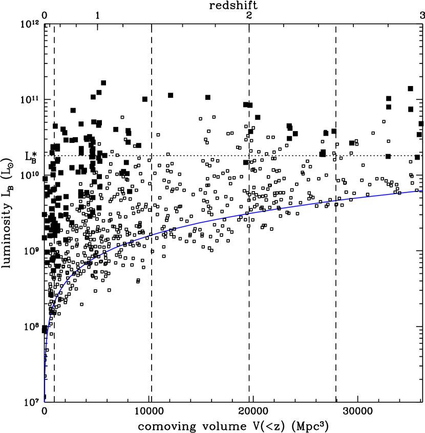
Figure 1: Rest–frame $B$–band luminosities of galaxies in the HDF–N plotted against redshift $z$ (top axis) or co–moving volume out to redshift $z$ (bottom axis). Filled symbols indicate galaxies with spectroscopic redshifts, while open symbols are galaxies with photometric redshifts only. The horizontal dotted line marks the luminosity of a present–day $L^{\ast}_{B}$ galaxy from the 2dFGRS luminosity function (Norberg et al., 2002). Vertical dashed lines divide the four redshift intervals used for analysis in this paper, each of which encloses approximately $10^{4}$ Mpc^-3. The curve indicates an approximate completeness limit for the sample for a magnitude limit of $\hbox{$H_{160}$}=26.5$ and assuming a spectral energy distribution that is constant in $f_{\nu}$ flux density.

Figure 1 shows the rest-frame $B$–band luminosities of HDF–N galaxies as a function of redshift $z$ (top axis), and of the co–moving volume out to redshift $z$ (bottom axis). This plotting scheme has the virtue that the horizontal density of points shows the co–moving space density of objects. The rest–frame $B$–band luminosities were computed by interpolating between the fluxes measured in the 0.3-2.2$\mu$m observed bandpasses. We converted to solar units assuming a $B$–band specific luminosity for the Sun of $L_{\nu,\odot}(B)=3.17\times 10^{18}$ erg s^-1 Hz^-1. The curve in Figure 1 shows an approximate completeness limit for the NICMOS sample, assuming a magnitude limit $\hbox{$H_{160}$}<26.5$ and a flat–spectrum $f_{\nu}$ spectral energy distribution. Roughly speaking, the upper envelope of galaxy luminosities is similar for $0<z<3$. The most optically luminous galaxy in the HDF–N is a red, giant elliptical FR I radio galaxy at $z=1.050$ (4-752), although another (possibly binary) galaxy at $z=2.931$ (4–52) comes close.

Although bright galaxies have similar space densities in the HDF–N out to $z=3$, their stellar populations do not remain the same. Figure 2 presents the rest–frame UV–optical colors of HDF–N galaxies versus redshift, showing a strong trend toward bluer colors at higher redshift. This effect cannot be attributed to selection biases because the sample is selected at near–infrared wavelengths. All points shown in Figure 2 are measurements, not limits; no object from the NICMOS sample studied here is undetected in the WFPC2 HDF–N. For galaxies at $z\sim 2.7$, the rest–frame 1700–$B$ color is approximately matched by the observed $V_{606}-H_{160}$. For the range of galaxy magnitudes we find at that redshift ($23\lesssim H_{160}<26.5$), we could have measured colors as red as $6\gtrsim V_{606}-H_{160}>4$, but none are found. The trend toward bluer colors at higher redshift presumably reflects a tendency toward younger stellar populations and increasing levels of star formation in more distant galaxies. As noted by PDF, nearly all HDF–N galaxies at $z>2$ have colors much bluer than those of present–day Hubble sequence galaxies, more similar to those of very active, UV–bright starburst galaxies. We may thus expect that the typical stellar mass–to–light ratios are lower for galaxies at higher redshift.

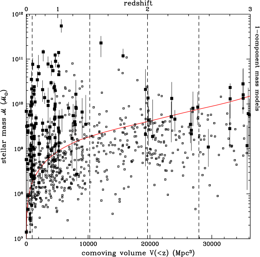
Figure 3: Estimates of stellar mass for HDF–N galaxies versus co–moving volume or redshift. Symbols are as in Figure 1. The mass estimates use Bruzual & Charlot models with solar metallicity and the 1–component star formation histories ($\Psi(t)\sim\exp(-t/\tau)$) described in the text. Error bars showing 68% confidence ranges are shown for the spectroscopic sample only in order to avoid overcrowding the figure. Masses estimated from lower metallicity models are generally somewhat smaller, while the “maximum $\hbox{$\mathcal{M}$}/L$” 2–component star formation histories yield larger masses, especially for the objects at higher redshift. The general character of the diagram remains the same, however, whichever models are used. The curve shows the mass corresponding to a maximally old stellar population, formed in a burst at $z=\infty$ and aging passively, with $\hbox{$H_{160}$}=26.5$. The NICMOS sample should be complete for all galaxies with stellar masses above this line. Galaxies younger and bluer than this maximally old model can be detected to lower mass limits.

Figure 3 shows the best–fitting stellar mass estimates for HDF–N galaxies, calculated using the 1–component (i.e., single exponential) SFR history models described in §3. Unlike the luminosities plotted in Figure 1, the upper envelope of galaxy masses declines markedly at higher redshift, and the space density of massive galaxies (say, $\hbox{$\mathcal{M}$}>10^{10}\hbox{$\mathcal{M}$}_{\odot}$) thins out. PDF found that the characteristic stellar mass of HDF–N LBGs is $\sim 10^{10}\hbox{$\mathcal{M}$}_{\odot}$. Even using a complete, infrared–selected, photometric redshift sample (which should be free of rest–frame UV selection biases), we do not find additional galaxies at similarly large redshifts with stellar masses greater than those of the bright HDF–N LBGs. The curve in the figure shows the stellar mass corresponding to a maximally old, red stellar population formed at $z=\infty$, aging passively, with $\hbox{$H_{160}$}=26.5$. The NICMOS sample should be complete for galaxies with $\hbox{$\mathcal{M}$}>10^{10}\hbox{$\mathcal{M}$}_{\odot}$ nearly out to $z=3$. At any redshift, some galaxies below this curve – those objects that are bluer than the maximum–$\hbox{$\mathcal{M}$}/L$, passive evolution limit – can be detected. However, we cannot rule out the possibility that we are missing faint, red, fading galaxies with masses that fall below the curve in Figure 3, but which might be too faint to detect in the NICMOS images.

As discussed in §3, we may set an upper bound on the stellar masses by adopting 2–component SFR models which include a maximally old component formed at $z=\infty$. This has a greater effect on the masses of the galaxies at higher redshift, where the observed colors are generally bluer and the photometric measurements do not reach as far to the red in the galaxy rest frame. Nevertheless, the basic character of Figure 3 remains the same even when these “maximal” mass estimates are used. Even with the maximum $\hbox{$\mathcal{M}$}/L$ models, very few galaxies at $z>1.4$, and no galaxies at $2<z<3$, have $\hbox{$\mathcal{M}$}>10^{11}\hbox{$\mathcal{M}$}_{\odot}$. Using either SFR model, the most massive galaxy in the HDF–N is the $z=1.05$ gE 4-752.0, and the most distant galaxy with $\hbox{$\mathcal{M}$}>10^{11}\hbox{$\mathcal{M}$}_{\odot}$ is the gE host galaxy (4-403.0) of the $z\approx 1.75$ type Ia supernova SN1997ff (Gilliland, Nugent & Phillips, 1999; Riess et al., 2001).

We will not discuss galaxies at $z>3$ in this paper because the NICMOS data do not probe the rest–frame optical light at those redshifts. However, one object which warrants special attention is the “$J$–dropout” object J123656.3+621322 (Dickinson et al., 2000), which has the reddest near–infrared colors of any object in the HDF–N. Its redshift is unknown; it might conceivably be an LBG or QSO at $z>12$, a dusty object at intermediate redshift, or an evolved galaxy with an old stellar population at high redshift. This latter possibility is most relevant here, as it might imply a large stellar $\hbox{$\mathcal{M}$}/L$. If we adopt a best–fit $z_{phot}=3.3$ for this object (excluding the $z>12$ option), we find that this object can be fit with an old ($\sim 1.6$ Gyr) stellar population with moderate dust extinction (required to match the red $J-H$ color – cf. Dickinson et al. (2000)), and $\hbox{$\mathcal{M}$}\approx 1\times 10^{11}\hbox{$\mathcal{M}$}_{\odot}$. If this interpretation were correct, this object would be significantly more massive than any other HDF–N galaxy at $z>2$. The only other object at $z>3$ with a fitted $\hbox{$\mathcal{M}$}>10^{11}\hbox{$\mathcal{M}$}_{\odot}$ is a broad–line AGN (4-852.12, $z=3.479$), whose luminosity and colors are probably significantly affected by the active nucleus, and where stellar population model fitting is therefore inappropriate. The comparatively red (and X–ray luminous) galaxy HDFN J123651.7+621221, at $z_{phot}=2.7$ (see Figure 2), is fit with a modest $\hbox{$\mathcal{M}$}\approx 1.5\times 10^{10}\hbox{$\mathcal{M}$}_{\odot}$.

5 The global luminosity and stellar mass densities

The HDF–N is a very narrow pencil–beam survey along a single sight–line, and any statistical analysis of its most luminous or massive galaxies is subject to small number statistics and to density variations due to clustering. We therefore adopt a very crude approach here, dividing the volume at $0.5<z<3$ into four redshift bins with approximately equal co–moving volume $\approx 10^{4}$ Mpc³ each: $z_{l}$ to $z_{u}=0.5$–1.4, 1.4–2.0, 2.0–2.5, and 2.5–3.0. The co–moving volume at $0<z<0.5$ is $<1000$ Mpc³, and we do not consider galaxies in that redshift range further here, although nearly 40% of the lifetime of the universe elapses in that interval. Based on the 2dFGRS optical luminosity function of Norberg et al. (2002), in the local universe we would expect $\sim 12$ galaxies with $L\geq L_{B}^{\ast}$ in a volume of $10^{4}$ Mpc³. From the 2dF+2MASS stellar mass function of Cole et al. (2001), we would expect $\sim 6$ galaxies with $\hbox{$\mathcal{M}$}\geq\hbox{$\mathcal{M}$}^{\ast}(=1.4\times 10^{11}\hbox{$\mathcal{M}$}_{\odot})$ in the same volume.

Figure 4 shows the cumulative luminosity densities $\rho_{L}(>L_{B})$ from the local 2dF luminosity function and from the HDF–N redshift slices. The HDF–N data are deep enough so that the luminosity densities are roughly convergent within each redshift slice at the detection limit. In each redshift interval, we evaluate the integrated $B$–band luminosity density and its uncertainty in several ways. First, we obtain a direct estimate, without extrapolation to fainter luminosities, by summing the galaxy luminosities, weighted inversely by the volumes over which they could be detected (the $1/V_{max}$ formalism of Schmidt (1968)). For each galaxy, the maximum redshift to which it could be seen with $\hbox{$H_{160}$}<26.5$ is calculated, using the multiband photometry for each object to compute the $k$–corrections directly. Most galaxies are visible throughout their redshift slices $z_{l}<z<z_{u}$, but when $z_{max}<z_{u}$, then $z_{max}$ is used to compute the $1/V_{max}$ weighting. The volume–weighted luminosities are then summed, and the uncertainty in this value is estimated by bootstrap resampling. Second, we have fit Schechter (1976) functions to the number densities in $\log(L_{B})$ bins, estimating parameter uncertainties using Monte Carlo simulations where the numbers of objects per bin were varied within a Poisson distribution. The Schechter functions generally give acceptable fits, except for the lowest redshift interval, where reduced $\chi^{2}=2.1$, mainly due to an inflection at the faint end which has little impact on the integrated luminosity density. The individual Schechter function parameters, $\phi^{\ast}$, $L^{\ast}$, and $\alpha$, are moderately well constrained for the lowest redshift subsample ($0.5<z<1.4$), where 382 objects are used, spanning nearly a factor of 1000 in luminosity. The best–fitting Schechter function parameters for this redshift bin, expressed in the $b_{J}$ band (conventionally normalized to Vega) for comparison to local determinations, are $M^{\ast}_{b_{J}}=-20.47\pm 0.35+5\log h$, $\phi^{\ast}=(2.0\pm 0.5)\times 10^{-2}h^{3}$ Mpc^-3, and $\alpha=-1.16\pm 0.07$. The luminosity function parameters are more poorly determined at higher redshifts, but in general the integrated luminosity densities, $\rho_{L}=L^{\ast}\phi^{\ast}\Gamma(\alpha+2)$, are better constrained.

Table 1 presents the results of the luminosity density integration using both methods. At $z<2.5$, the Schechter function integrations yield values for $\rho_{L}$ which are within 0.1 dex of the direct sums, confirming that the HDF observations are detecting most of the light at those redshifts. In the highest redshift interval ($2.5<z<3$), our sample has only 45 galaxies spanning a range of $\sim 30$ in luminosity, and the Schechter function slope $\alpha$ is poorly constrained, leading to larger uncertainty in $\rho_{L}$; $>5$% of the Monte Carlo simulations lead to divergent $\rho_{L}$ (i.e., $\alpha<-2$). For the purposes of this analysis, we have refit the data in the highest redshift bin fixing the slope to $\alpha=-1.4$, the steepest value found in the lower redshift ranges, but still somewhat shallower than $\alpha=-1.6$ for the rest–frame UV luminosity function of LBGs (Steidel et al., 1999).

Our estimates of the rest–frame $B$–band luminosity density, along with various measurements from the literature, are shown in Figure 5. At $z\approx 1$, we find that $\rho(L_{B})$ is $\sim 2.5\times$ larger than that in the local universe ($\log(\rho_{L}/L_{\odot})=8.1$, Norberg et al. (2002)), consistent with previous results. The luminosity function and density are consistent with modest luminosity evolution (0.85 mag for rest–frame $L^{\ast}_{B}$) and 25% higher space densities ($\phi^{\ast}$) at $z\approx 1$ compared to the present day. At higher redshift ($1.4<z<3$), the luminosity density is roughly constant at $\sim 1.5\times$ the local value. However, we have seen that galaxies at higher redshift have bluer colors and presumably lower mass-to-light ratios. Hence, the density of stellar mass may be expected to evolve differently than that of the light.

To compute the stellar mass density in each redshift slice, we begin by summing the masses for everything that we can see, e.g., $\rho_{\ast}(>L_{B})$. As noted above, for the oldest possible stellar populations with maximum $\hbox{$\mathcal{M}$}/L$ we can only be certain of being complete down to the mass limits shown by the line in Figure 3. Thus we can confidently detect objects with $\hbox{$\mathcal{M}$}>4\times 10^{9}\hbox{$\mathcal{M}$}_{\odot}$ out to $z=2$ and $\hbox{$\mathcal{M}$}>10^{10}\hbox{$\mathcal{M}$}_{\odot}$ out to nearly $z=3$, but we cannot be completely certain that some objects with smaller masses but large $\hbox{$\mathcal{M}$}/L$ are not missed. As noted above, there is little evidence for a significant population of galaxies at $z>2$ with $\hbox{$\mathcal{M}$}/L$ much larger than that seen for LBGs, so it might be surprising if such a population were to appear fainter than the detection limit of the NICMOS data. Also, at all redshifts in the HDF–N sample, the mean $\langle\hbox{$\mathcal{M}$}/L\rangle$ is either declining or flat with decreasing $L_{B}$ (cf. Figure 1 from PDF, where a mild tendency toward bluer colors at fainter magnitudes is seen for LBGs at $2<z<3.5$). This is a well–known trend in the local universe (cf. Kauffmann et al. (2002)): fainter galaxies on average tend to have bluer colors and lower stellar $\hbox{$\mathcal{M}$}/L$. This effect would be even more pronounced if our stellar population modeling had incorporated a trend of increasing metallicity with mass or luminosity.

Parenthetically, it is worth noting that Shapley et al. (2001) have reported evidence for an extremely steep faint–end slope to the rest–frame optical luminosity function of LBGs at $z\approx 3$, as well as a tendency for fainter galaxies to have redder UV–optical colors, and hence presumably larger $\hbox{$\mathcal{M}$}/L$. These two trends are intimately connected in the Shapley et al. (2001) sample, since they infer the observed–frame $K_{s}$–band luminosity distribution from the observed ${\cal R}$–band data (with which Steidel et al. (1999) measured $\alpha_{UV}=-1.6$) and the ${\cal R}-K_{s}$ color distribution of galaxies in their sample. Taken at face value, these facts would imply a very large mass density of faint red galaxies at $z\approx 3$, below the magnitude limits of ground–based Lyman break galaxy surveys. The Shapley et al. (2001) sample, however, spans a limited range of luminosities, restricted to the bright end of the LBG distribution. It is very difficult to constrain the faint end slope with such data; we are unable to do so reliably even with our deeper NICMOS sample. Moreover, we find no such reddening trend with fainter magnitudes for HDF–N LBGs, pushing well below the magnitude limits of the ground–based samples. If anything, the opposite seems to be the case. For the moment, therefore, we discount this result from Shapley et al. (2001), but we stress the important caveat that even the deepest near–infrared data and photometric redshift samples presently available cannot definitely constrain these important properties of the galaxy distribution at $z>2.5$, leaving genuine uncertainty about the integrated stellar mass content at such redshifts.

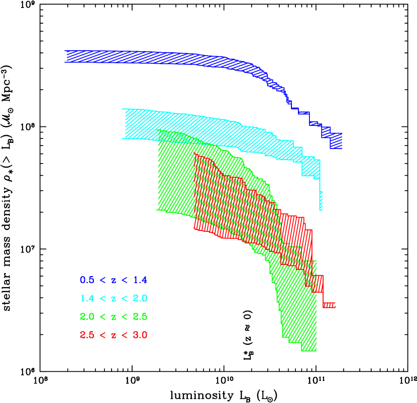
Figure 6: Cumulative stellar mass densities for HDF–N galaxies brighter than a given rest–frame $B$–band luminosity, in various redshift intervals. The hatched regions show the range of estimates using different stellar population models, going from low metallicity, 1–component $\Psi(t)$ models (lower bounds) to solar metallicity, 2–component “maximum $\hbox{$\mathcal{M}$}/L$” models (upper bounds).

The cumulative stellar mass density $\rho_{\ast}(>L_{B})$ in the four HDF–N redshift slices is presented in Figure 6. As discussed above, the fitted mass estimates depend on the model metallicities and on the adopted star formation histories. Here, we show the range of mass densities obtained by varying the model metallicities from 0.2 to $1.0\times Z_{\odot}$, and from the single and 2–component SFR history models. The dependence of the mass densities on these model assumptions is less than a factor of 2 at $z\sim 1$, but can be as much as a factor of 4 out at $z\sim 2.7$. At $z<2.5$, the mass densities are approximately convergent. At $z>2.5$, $\rho_{\ast}$ from the 1–component models appears to be converging, but is still rising for the 2–component, maximum $\hbox{$\mathcal{M}$}/L$ models. This is a consequence of the mass completeness limit drawn in Figure 3. Just as galaxies might be present, but undetected by NICMOS, with masses that fall below that curve, any faint galaxy that is detected may in principle have an unseen old stellar component with mass roughly equal to that shown by the completeness line. The maximum $\hbox{$\mathcal{M}$}/L$, 2–component models therefore permit the potential existence of a galaxy population with $\hbox{$\mathcal{M}$}/L\propto L_{B}^{-1}$ below some threshold mass set by the NICMOS detection limits.

For each redshift interval, we calculate the volume–averaged mass–to–light ratio $\langle\hbox{$\mathcal{M}$}/L\rangle$ by taking the ratio of the mass and $B$–band luminosity densities for the observed galaxy populations. Our calculations of $\langle\hbox{$\mathcal{M}$}/L\rangle$ under various stellar population assumptions are presented in Table 2. For comparison, the 2dFGRS measurements of Norberg et al. (2002) and Cole et al. (2001) yield a local value $\langle\hbox{$\mathcal{M}$}/L\rangle=4.4\hbox{$\mathcal{M}$}_{\odot}/L_{\odot}$. This is significantly larger than the values we derive at high redshift, implying substantial evolution in the mean stellar population properties (averaged over all galaxies) from $z\approx 1$ to the present. We multiply the computed $\langle\hbox{$\mathcal{M}$}/L\rangle$ values by our estimates of the total $\rho_{L}$ from the Schechter function integration described above. Note that if $\hbox{$\mathcal{M}$}/L$ decreases at fainter luminosities, this procedure will slightly overestimate the stellar mass density. The random uncertainty in $\rho_{\ast}$ is estimated from the combined uncertainties in $\rho_{L}$ and the quadratic sum of the mass fitting uncertainties (for each particular choice of model metallicity and $\Psi(t)$) for the galaxies in each redshift range. The systematic dependence of the results on these choice of stellar population model assumptions is illustrated below, and our results are tabulated in Table 3. Note that we have used the rest–frame $B$–band primarily as an accounting device here, calculating $\langle\hbox{$\mathcal{M}$}/L_{B}\rangle$ and using a Schechter fit to the luminosity function to correct for sample incompleteness at the faint end. Our stellar masses are actually derived using NICMOS and ground–based near–IR observations that reach significantly redder rest–frame wavelengths (0.54–1.44$\mu$m for the $K_{s}$–band data) over the entire redshift range being considered here.

Regardless of the model adopted for the mass estimates, there is good evidence that the global stellar mass density increased with cosmic time. E.g., for galaxies brighter than present–day $L^{\ast}_{B}$, which are abundant in the HDF–N at all redshifts $z<3$, the minimum estimate for $\rho_{\ast}$ at $z\approx 1$ is $\sim 7\times$ larger than that from the maximum $\hbox{$\mathcal{M}$}/L$ models at $z\approx 2.7$.

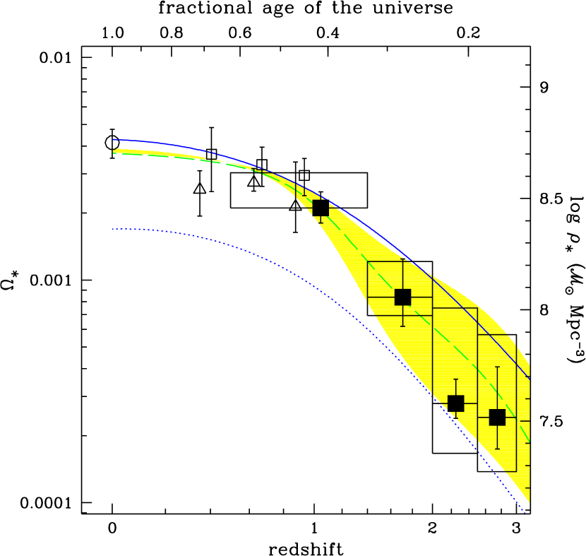
Figure 7: The redshift evolution of the co–moving stellar mass density, $\Omega_{\ast}$. The horizontal axis scaling and error bars are as in Figure 5. Open symbols show results from the literature at $0<z<1$ (circle – Cole et al. (2001); triangles – Brinchmann & Ellis (2000); squares – Cohen (2002)). The HDF–N points (large filled squares) show results for the $Z_{\odot}$, 1–component $\Psi(t)$ model fits. The vertical error bars show the 68% random errors for this choice of model, combining the sampling variance and the mass fitting uncertainties. The vertical extent of the boxes show the range of systematic uncertainty introduced by varying the metallicity and the star formation histories of the mass–fitting model. The blue curves show the result of integrating the cosmic star formation history SFR($z$) traced by rest–frame UV light, with and without corrections for dust extinction (solid and dotted curves). The dashed green curve shows the integrated star formation history from Pei, Fall & Hauser (1999), with their 95% confidence range indicated by the shaded region.

Figure 7 places the HDF–N mass density estimates into a global context, comparing them with other data at $0<z<1$, where the HDF–N itself offers little leverage due to its small volume. The local stellar mass density is taken from Cole et al. (2001), integrating over their fit to the stellar mass distribution of 2dFGRS galaxies. This value is consistent with earlier estimates by Fukugita, Hogan & Peebles (1998) and Salucci & Persic (1999), but has smaller statistical uncertainties. Values at $0.3<z<1$ are taken from Brinchmann & Ellis (2000) and Cohen (2002), with adjustment for the change in cosmological parameters to those adopted here. Our own estimates of $\Omega_{\ast}$, as well as those of Cole et al. (2001) and Cohen (2002), integrate over luminosity functions to estimate the total luminosity and mass densities. Brinchmann & Ellis (2000) computed $\rho_{\ast}$ by summing over galaxies in the range $10.5<\log(\hbox{$\mathcal{M}$}/\hbox{$\mathcal{M}$}_{\odot})<11.6$, without extrapolating further down an assumed mass function, and thus their published values are strictly lower limits. Those authors estimate that their summation accounts for $\geq 80$% of $\rho_{\ast}$, and we have therefore applied a 20% upward correction to their points to roughly account for this incompleteness. Note also that Cole et al. (2001) fit metallicities for each galaxy, primarily based on near–infrared colors. From their Figure 11, it appears that most 2dFGRS galaxies are best fit with models close to solar metallicity, and generally not lower than $Z=0.004$. Brinchmann & Ellis (2000) also allow metallicity to vary from 0.004 to 0.02 in their mass fitting, while Cohen (2002) adopt evolutionary corrections based on population synthesis models from Poggianti (1997), which include chemical evolution. We have found (see PDF) that we cannot set reliable photometric constraints on metallicity for the higher redshift galaxies, and therefore have used different (but fixed) values to explore the systematic dependence of $\rho_{\ast}$ on $Z$.

6 Discussion

6.1 The evolution of the global stellar mass density

At $z\approx 1$, we find that 50–75% of the present–day stellar mass density had already formed, depending on the stellar population models adopted. Our estimates are consistent with those from Brinchmann & Ellis (2000) and Cohen (2002), who studied larger samples over greater volumes at $0.3<z<1$. Our HDF–N analysis alone does not offer sufficiently fine redshift resolution to further pin down the epoch when (e.g.) 50% of the stars in the universe had formed, but it seems to have taken place somewhere in this range.

At $z>1.4$, we see a steep drop in the total stellar mass density with increasing redshift. The systematic uncertainties in our mass estimates are large at $z>2$, primarily because the NICMOS near–infrared measurements sample only rest–frame optical wavelengths in the $B$– to $V$–band range, loosening our constraints on $\hbox{$\mathcal{M}$}/L$. In addition, even these NICMOS observations do not go deep enough to tightly constrain the luminosity function at $z>2.5$, although a fairly robust estimate of the luminosity density can be made with only modest and reasonable constraints on the faint end slope $\alpha$. Nevertheless, the apparent change in the stellar mass density is sufficiently dramatic as to exceed the substantial uncertainties in the measurements. For our fiducial stellar population models with solar metallicity and exponential star formation histories, the mass density changes by a factor of 17 from $z\approx 2.7$ to the present–day. Even for the “maximum $\hbox{$\mathcal{M}$}/L$” 2–component models, $\rho_{\ast}$ is $\sim 7\times$ smaller at $z\approx 2.7$ than at $z=0$. Even if all galaxies in the highest redshift bins were set at their 68% upper confidence limits of their mass estimates for this model, we would find less than 1/3rd of the present–day mass density present.

The quantity $\rho_{\ast}(z)$ is essentially the time integral over the cosmic star formation history SFR($z$) = $\dot{\rho}_{\ast}(z)$. The blue curves in Figure 7 show the integral over SFR($z$) inferred from rest–frame UV light (e.g., Lilly et al. (1996); Madau, Pozzetti & Dickinson (1998); Steidel et al. (1999)), using parameterized fits given by Cole et al. (2001) (extrapolated to $z_{max}=7$). The integration incorporates the time–dependent recycling of stellar material back to the ISM from winds and supernovae, following the relation for a Salpeter IMF and solar metallicity calculated with the Bruzual & Charlot models. Asymptotically, this recycled fraction $R=0.32$ at age = 13 Gyr.

It is now widely believed that measurements based on rest–frame UV light underestimate the total rate of high redshift star formation unless corrections for dust extinction are included. This can also be seen from the integrated stellar mass, $\Omega_{\ast}(z)$, as well. The curves in Figure 7 show the integrated SFR($z$) with and without nominal corrections for dust extinction taken from Steidel et al. (1999). As Madau, Pozzetti & Dickinson (1998) and Cole et al. (2001) have previously noted, without the boost from an extinction correction, this integral results in a present–day mass density which is substantially smaller than the observational estimates. Here, we can see that this is true over the broader redshift range $0<z<3$, although at $z>2$ the inconsistency is small given the systematic uncertainties in $\rho_{\ast}$. On the other hand, the extinction–corrected SFR($z$) results in $\rho_{\ast}(z)$ which agrees fairly well with observations at $z\approx 0$ and $z\approx 1$, but which exceeds our best estimates at higher redshifts. Again, given the modeling uncertainties, these estimates are consistent with the upper bounds from the maximum $\hbox{$\mathcal{M}$}/L$ models, but as noted above, this class of mass models is somewhat unrealistic and inconsistent when considered over a wide range of redshifts. The parameterized SFR($z$) from Cole et al. (2001) rises by a factor of $\approx 2$ from $z=4$ to its peak at $z\approx 1.5$. A flatter star formation history at $z>2$ would exacerbate this discrepancy.

Pei, Fall & Hauser (1999) have used measurements of the UV luminosity density and neutral gas density as a function of redshift and the far–infrared background to constrain a self–consistent solution for the global star formation history. Their solution (from their Figure 12), converted to our adopted cosmology, is shown as the green solid curve in Figure 7, while the shaded region shows their 95% confidence interval. The result and its uncertainty range are in impressively good agreement with the data (and their uncertainties) at all redshifts, providing encouragement that these different observables can be united within a common framework for galaxy mass assembly at $0<z<3$.

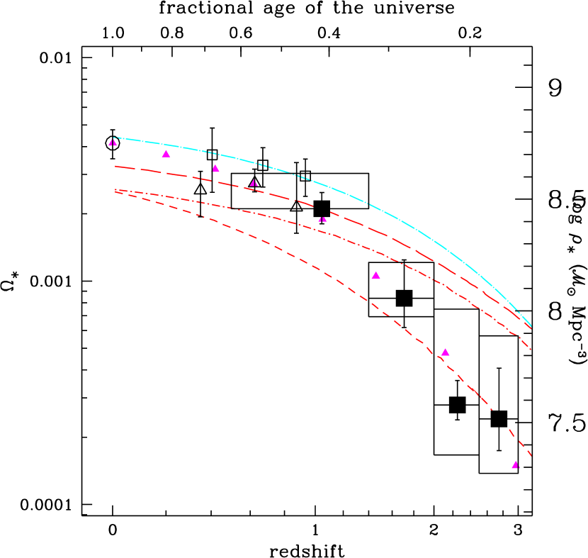
Figure 8: Same as Figure 7, with curves showing $\Omega_{\ast}(z)$ from semi–analytic galaxy evolution models by Cole et al. (2000) (cyan dot–long-dashed) and Somerville et al. (2001) (red long–dashed: “collisional starburst”; dot–short-dashed: “accelerated quiescent”; short–dashed: “constant quiescent”). The small, filled magenta triangles show results from combined $N$–body and semi–analytic models by Kauffmann et al. (1999), rescaled to match the observed $z=0$ mass density. As discussed in the text, these are probably lower limits to the total $\Omega_{\ast}$ at high redshift.

Figure 8 reproduces the data points from Figure 7, superimposing results for $\Omega_{\ast}(z)$ from recent semi–analytic models of galaxy evolution by Cole et al. (2000) and Somerville et al. (2001). These models use the same cosmological parameters as we have adopted here. The calculations of Cole et al. (2000) used the IMF of Kennicutt (1983). We have approximately rescaled to a Salpeter IMF by multiplying $\rho_{\ast}(z)$ by a factor of 2. We also shows results from the $N$–body plus semi–analytic models of Kauffmann et al. (1999). Because of their mass resolution, these model outputs (taken from the Virgo Consortium web site) are limited to stellar masses $\hbox{$\mathcal{M}$}>10^{10}\mathcal{M}_{\odot}$ at $z>1.4$ and $\hbox{$\mathcal{M}$}>2\times 10^{10}\mathcal{M}_{\odot}$ at $z<1.4$. This is similar to the characteristic stellar mass of LBGs at high redshift, and thus a large extrapolation would be required to estimate the total $\rho_{\ast}$. We fit the slope of the differential mass function in the models and integrated to compute the stellar mass density $\rho_{\ast}(>10^{10}\mathcal{M}_{\odot})$ at all redshifts, but have not extrapolated further. Kauffmann et al. (1999) assume the IMF of Scalo (1986), requiring an additional adjustment, possibly redshift dependent, for comparison to our assumed Salpeter IMF. Very roughly, we have accounted for this, as well as for the extrapolation to “total” integrated $\Omega_{\ast}$, by simply rescaling the model $\rho_{\ast}$ so that it matches the value from the 2dFGRS at $z=0$.

In the model of Cole et al. and the favored “collisional starburst” model of Somerville et al., the peak redshift for star formation is at $z\approx 2.5$ to 4. Hence, these models show somewhat flatter evolution of $\Omega_{\ast}(z)$, with a larger fraction of the stars in the universe formed at $z>1.5$ than our data suggest. Kulkarni & Fall (2002) have noted that some semi–analytic models also overpredict the mean metallicity in damped Lyman $\alpha$ absorption line systems at high redshift, for similar reasons. Star formation in the “constant quiescent” model of Somerville et al. peaks at lower redshift ($z\approx 1.5$), yielding better agreement with the high redshift data, but underpredicting $\Omega_{\ast}$ at $0<z<1.5$. The model of Kauffmann et al. (1999) (after rescaling to match the data at $z=0$) appear to match the shape of $\Omega_{\ast}(z)$ somewhat better than do the other models. However, given the shapes of the mass functions in their simulations, one would expect that a proper extrapolation to total $\rho_{\ast}$ would have a larger effect at higher redshifts. This would most likely flatten the $\Omega_{\ast}(z)$ evolution somewhat, and therefore the higher redshift points from the Kauffmann et al. models should probably be regarded as lower limits.

Broadly speaking, our estimates of $\Omega_{\ast}(z)$ favor a global star formation history whose rate peaks at $1<z<2$ and is smaller at higher redshift. A higher peak redshift for SFR($z$), or a flat rate out to $z\gg 3$, would appear to be inconsistent with our measurements, producing too many stars at $2<z<3$ relative to the mass density at lower redshifts. Ferguson, Dickinson & Papovich (2002) have noted a conflict between the stellar mass content inferred for $z\sim 3$ LBGs and the evidence for substantial amounts of star formation at higher redshifts, as seen directly in the $z\sim 4$ LBG population, or as implied by the radiation required to reionize the Universe at $z>6$. A constant rate of star formation at $3<z<6+$ would overpredict the stellar masses of LBGs at $z\approx 3$, as well as $\Omega_{\ast}$ at that redshift.

Neither the current data, nor the theoretical predictions, are yet sound enough to imply a definite paradox. If necessary, however, there may be several ways to reconcile our measurements of $\Omega_{\ast}(z)$ with evidence for larger star formation rates at higher redshift. First, we might have underestimated luminosity or mass densities at high redshift. For example, Lanzetta et al. (2002) have suggested that failure to account for surface brightness dimming has led to underestimates in the UV luminosity density, and hence the star formation rate, at high redshift. Although we stress that we have not used isophotal photometry here, virtually any photometry scheme is subject to some biases, and we might nevertheless have underestimated the near–IR fluxes (and hence masses) of high–$z$ objects. We may also be missing light from a population fainter than our NICMOS detection limits, either due to a steep upturn in the luminosity function, or because of a steep increase in $\hbox{$\mathcal{M}$}/L$ at fainter luminosities. We note that surface brightness biases would quite probably affect estimates of both SFR($z$) and $\rho_{\ast}(z)$ in similar ways, so that the inconsistency might not be significantly narrowed even if corrections were made for missing light. The results on $\rho_{\ast}(z)$ do not allow much room for substantially higher rates of star formation at high redshift, either due to surface brightness effects or dust obscuration, unless the stellar mass estimates are also grossly underestimated.

It is also possible that our assumption of a constant IMF at all redshifts could be wrong. One solution proposed by Ferguson et al. is to tilt the IMF toward massive star formation at higher redshifts. With a flatter IMF, the massive stars that would produce UV radiation at the reionization epoch, or from LBGs at $z\approx 4$, are accompanied by a smaller total formation rate of stellar mass, which is dominated by lower–mass, long–lived stars. In this way, we may reconcile the UV output at $z\gg 3$ with the relatively low $\Omega_{\ast}$ seen at $2<z<3$. Eventually, however, there must be a change in the IMF to produce the longer–lived stars which dominate the stellar mass build–up at $1<z<3$. It is not clear how to realistically incorporate a time– or redshift–dependent IMF into current models of galaxy evolution, but this may become necessary.

It is also interesting to note the relative paucity of galaxies with $\hbox{$\mathcal{M}$}>10^{11}\hbox{$\mathcal{M}$}_{\odot}$ at almost any redshift in the HDF–N (see Figure 3). Cole et al. (2001) find a characteristic stellar mass of present–day galaxies $\hbox{$\mathcal{M}$}^{\ast}=1.4\times 10^{11}\hbox{$\mathcal{M}$}_{\odot}$. There are only a handful of HDF–N galaxies at $0.5<z<2$ which exceed this mass, despite adequate total volume to have found roughly a dozen in the local universe. This is true even when the maximum $\hbox{$\mathcal{M}$}/L$ 2–component star formation models are adopted for the HDF–N galaxies. This might be attributable to small number statistics and to the small co–moving volume of the HDF–N. The most massive galaxies are rare, and moreover they may be expected to cluster strongly, making it still more difficult to take a fair census from a single sight line, small–volume survey. However, it might also indicate that the most massive galaxies continued to build up their stellar content at relatively late epochs, either by merging or late star formation, even after the time when much of the overall density of stars in the universe had already formed.

Although we cannot yet derive robust stellar mass functions at high redshift from our data, the qualitative behavior seen in Figure 3 is reminiscent of that found in recent cold dark matter models of galaxy formation in a $\Lambda$–dominated universe. Baugh et al. (2002) show stellar mass functions at various redshifts derived from the models of Cole et al. (2000), and similar results can be extracted from the models of Kauffmann et al. (1999) available from the Virgo Consortium web site. Locally, galaxies with stellar masses $\hbox{$\mathcal{M}$}\approx 10^{11}h_{70}^{-2}\mathcal{M}_{\odot}$ have a space density $\phi\approx 2\times 10^{-3}h_{70}^{-3}$ Mpc^-3. We consider objects at a fixed space density corresponding to that of $10^{11}\hbox{$\mathcal{M}$}_{\odot}$ galaxies at $z=0$. In both sets of models, at $z\approx 1$, 2, and 3, the stellar mass of objects with this characteristic space density has decreased by factors of $\sim 2$, 4, and 10, respectively. At $z=3$, the characteristic mass is approximately $10^{10}\hbox{$\mathcal{M}$}_{\odot}$, as found by PDF. The models differ in their predictions for the space density of $10^{11}\hbox{$\mathcal{M}$}_{\odot}$ objects, with Baugh et al. (2002) finding more rapid evolution. This is unsurprising in the exponential part of the mass function, where small differences along the mass axis correspond to very large differences in space density. Both models, however, predict that $\phi(10^{11}\hbox{$\mathcal{M}$}_{\odot})$ changes by more than an order of magnitude between $z=2$ and 1, and that galaxies with that mass largely disappear by $z=3$, with a space density less than 1% of that locally.

Although we find no HDF–N galaxies at $z>2$ with $\hbox{$\mathcal{M}$}>10^{11}\mathcal{M}_{\odot}$, this does not mean that such galaxies do not exist in the Universe. Shapley et al. (2001) find a small number of LBGs with inferred $\hbox{$\mathcal{M}$}\gtrsim 10^{11}\hbox{$\mathcal{M}$}_{\odot}$ among a sample taken from their large, ground–based survey. Moreover, there are powerful radio galaxies in this redshift range with substantially brighter $K$–band magnitudes, and presumably larger stellar masses, than anything in the HDF–N (c.f. De Breuck et al. (2002)). Overall, however, galaxies with these large stellar masses at $z\approx 3$ appear to be quite rare. Wide–field (but deep) near–infrared surveys with reliable redshift information will be needed to quantify this properly.

From large redshift surveys of $K$–selected galaxy samples, Cohen (2002) and Cimatti et al. (2002b) have argued that the galaxies which make up the bulk of the stellar mass distribution today have evolved in a fashion that is broadly consistent with pure luminosity evolution, at least from $z\approx 1$ or 1.5 to the present. We see little evidence to contradict this from the HDF–N. The difference in luminosity density from $z\approx 1$ to the present is broadly consistent with “passive” luminosity evolution ($\sim 0.85$ mag in rest–frame $L^{\ast}_{B}$) with only modest ($\sim 25\%$) density evolution (see §5). At higher redshift, however, our results would strongly disagree with simple prescriptions for pure luminosity evolution.

6.2 Field–to–field variations

Our present analysis is limited to one very deep, but very small, field of view, and is therefore subject to uncertainties due to the relatively small co–moving volume and the effects of galaxy clustering. We have quantified the shot–noise uncertainties, but we have made no attempt to deal with the possible influence of clustering, other than to use very wide redshift intervals when analyzing the data in the hope of averaging over line–of–sight variations. Although the co–moving volume of each of our redshift bins is roughly equal, the co–moving, line–of–sight path–length ranges from $2300h_{70}^{-1}$ Mpc at $0.5<z<1.4$ to $530h_{70}^{-1}$ Mpc at $2.5<z<3$. We know that the redshift distributions of galaxies at both low and high redshift exhibit “spikes,” as pencil–beam surveys penetrate groups and sheets along the sight–line (cf. Le Fèvre et al. (1996), Cohen et al. (1996), Adelberger et al. (1998)). We would expect our redshift bins to average over several of these overdensities and the “voids” between them. Nevertheless, we may expect that clustering will introduce some additional variance, beyond that included in our error estimates. Indeed, it may be expected that the most massive galaxies cluster most strongly at any redshift.

One motivation for the Hubble Deep Field South project (HDF–S, Williams et al. (2000)) was to provide a cross–check on results from the HDF–North, as insurance against “cosmic variance”. Rudnick et al. (2001) have presented deep, near–infrared observations of the HDF–S from the VLT. To date, few spectroscopic redshifts are available in the HDF–S, but Rudnick et al. have estimated photometric redshifts and rest–frame optical luminosities for galaxies in their sample. They find 6 galaxies in the HDF–S with $2<z_{phot}<3$ and $L_{B}>10^{11}h_{70}^{-2}L_{\odot}$ whereas we find two in the HDF–N. These differences may be within the range expected from statistical fluctuations, which have already been taken into account by our bootstrap error analysis of the luminosity density, although larger variance due to clustering (particularly for the most luminous objects) are to be expected. The most luminous HDF–S galaxies at $2<z_{phot}<3$ are about twice as bright as those in the HDF–N. It is important to remember, however, that for distributions like the Schechter function, the objects that contribute most to the total luminosity or mass density are those around $L^{\ast}$ or $\hbox{$\mathcal{M}$}^{\ast}$, i.e., the “typical” objects, not the brightest ones. Labbé et al. (2002) identify 7 HDF–S galaxies with $1.95<z_{phot}<3.5$ and with $V-H$ colors redder than galaxies at similar redshift in the HDF–N (cf. PDF Figure 1). If the HDF–S photometric redshift estimates are correct, then these galaxies may have higher $\mathcal{M}/L$ than the large majority of galaxies with similar redshifts and $B$–band luminosities in either the northern or southern fields.

The differences between the HDF–S and HDF–N may be actually be greater at $0.5<z<2$, where Rudnick et al. (2001) find no galaxies with $L_{B}>10^{11}h_{70}^{-2}L_{\odot}$, compared to six in the HDF–N. The fact that the HDF–N luminosity density at $z\approx 1$ agrees well with that measured in other surveys that cover wider fields or multiple sight lines gives us some confidence in our mass density estimates at that redshift. At $1.4<z<2$, where both samples rely very heavily on photometric redshifts, Rudnick et al. find only two HDF–S galaxies with $L_{B}>2\times 10^{10}h_{70}^{-2}L_{\odot}$ (roughly present–day $L_{B}^{\ast}$), compared to 17 in the HDF–N. Overall, these comparisons point to the need for caution interpreting results from any one deep, narrow survey, and highlight the importance of wider fields of view and multiple sight lines.

6.3 Photometric redshift errors

Many of the galaxies in the HDF–N have only photometric redshift estimates. It is therefore important to consider the effects of photometric redshift errors on our results. At all redshifts, the brighter galaxies make up a substantial fraction of the total stellar mass density, and in the HDF–N most of these have spectroscopic redshifts. For the range of model metallicities and star formation histories that we have considered, the fraction of $\log\rho_{\ast}$ that is made up by objects with spectroscopic redshifts in each of our redshift bins is: $0.5<z<1.4$ – 74-78%; $1.4<z<2.0$ – 35-43%; $2.0<z<2.5$ – 22-28%; $2.5<z<3.0$ – 32-41%. Photometric redshift errors are therefore unlikely to have a dominant effect on mass densities at $z\approx 1$, but may be more important at higher redshifts.

Photometric redshift errors come in two “flavors”: small uncertainties, and catastrophic outliers (§2). To first order, small redshift errors translate quadratically to changes in luminosity and hence to the derived masses. We have perturbed our photometric redshifts by amounts drawn from the observed $\Delta_{z}$ distribution for the spectroscopic sample, truncated at $|\Delta_{z}|<0.1$. Objects with spectroscopic redshifts were not perturbed. The changes in $\log\rho_{L}$ within each redshift bin are small. Averaging over many perturbations, the mean and RMS offsets range from $-0.006\pm 0.003$ dex at $0.5<z<1.4$ to $+0.05\pm 0.03$ dex at $2.5<z<3$, and are smaller than other computed uncertainties.

A greater concern is the possibility of catastrophic outliers. The most common cause is aliasing between minima in $\chi^{2}(z_{phot})$, e.g., from confusion between different breaks or inflections in the spectral energy distribution. In such cases, it is possible to mistake a faint, low–redshift object for a very luminous one at high redshift. Moreover, the rest–frame colors, and hence $\hbox{$\mathcal{M}$}/L$ derived from spectral model fitting, could be completely wrong. A moderately red galaxy at low redshift, if incorrectly assigned a large $z_{phot}$, might be fit with a very red, high–$\hbox{$\mathcal{M}$}/L$ stellar population, or we might miss a massive, red, high–$z$ galaxy if it were erroneously placed at low $z_{phot}$. The impact of such errors is largest at higher redshifts. Transferring a few galaxies between (say) $z_{phot}<1.4$ and $2<z<3$ will have relatively little effect on global quantities at low redshift (where their inferred luminosities would be small), but might cause a significant change in the high redshift bins.

It is difficult to assess the impact of such catastrophic redshift errors formally, but we have looked closely at the situation in the HDF-N, and offer the following observations. The largest effect would most likely be due to redshift errors for galaxies with relatively bright near–infrared magnitudes. Only 18 (out of 107) HDF–N galaxies with $\hbox{$H_{160}$}<23$ lack spectroscopic redshifts. These 18 galaxies all have best–fitting $0.9<z_{phot}<1.8$. Examining the photometric redshift likelihood function for each, we find that four have next–best values in the range $2<z_{phot}<3$. In three of the four cases, $\chi^{2}$ for the next–best $z_{phot}$ is 45 to 125$\times$ poorer than that of the best fit. The morphologies and SED shapes strongly suggest that these are ordinary, early–type galaxies at $1.1<z<1.2$. One galaxy (4-186) is more problematic. It is best fit by $z_{phot}=1.71$ (Fernández-Soto et al. (1999) find a very similar $z_{phot}=1.60$), but $\chi^{2}$ is only $2.5\times$ worse at $z_{phot}=2.86$. We see no reason to doubt the best–fit value, but this is an example of a galaxy which might, in principle, be at higher redshift. With $\hbox{$H_{160}$}=22.2$ and red colors, its stellar mass would be much larger if placed at the higher redshift. At $23<\hbox{$H_{160}$}<24$ there are five more galaxies with best–fit $z_{phot}<2$ and next–best $2<z_{phot}<3$. For three, the next–best $\chi^{2}(z_{phot})$ values are again far worse, and careful inspection makes $z>2$ seem unlikely. Two others have smaller $\chi^{2}$ ratios, and for one (3-515.11), both possibilities ($z_{phot}=1.24$ or 2.64) seem comparably likely, with $\chi^{2}$ differing by a factor of only 1.2. At the larger redshift, this would be a fairly ordinary, $\sim L^{\ast}$ LBG with blue colors and typical $\hbox{$\mathcal{M}$}/L$, and would only slightly increase the global $\rho_{M}$. At still fainter magnitudes, a modest rate of catastrophic errors would have very little effect on the global mass densities.

In another test, we compared two somewhat different photometric redshift fits: one (the default for this paper) using the WFPC2+NICMOS+IRIM photometry and “trained” spectral templates from Budavári et al. (2000), versus another which excludes the ground–based $K$–band data and uses more conventional templates based on the Coleman, Wu & Weedman (1980) empirical SEDs. Only one blue, faint galaxy shifted into or out of the range $2<z_{phot}<3$, with negligible impact on luminosity or mass densities. Finally, our photometric redshift estimates can optionally incorporate a constraint on rest–frame $B$–band luminosity, somewhat similar to the Bayesian priors used in the method of Benítez (2000). This might, in principle, cause erroneous $z_{phot}$ estimates for unusually luminous galaxies at high redshift. However, when we switch off this luminosity prior, no galaxy is reassigned to $2<z_{phot}<3$, and there is no significant effect on our results.

Without reliable spectroscopic redshifts for all galaxies, we cannot be absolutely certain that photometric redshift errors do not affect our derived luminosity or mass densities. However, from the tests performed here we see no strong evidence that this is a significant problem for the HDF–N sample. It is important, however, to remember that for some questions, a comparatively small error rate in photometric (or spectroscopic) redshifts can introduce potentially large errors in the derived results. Other problems (e.g., galaxy clustering) are more robust against modest redshift error rates.

7 Conclusions

We have used deep near–infrared imaging of the Hubble Deep Field North to select a sample of galaxies based on their optical rest–frame light out to $z=3$, and have estimated their stellar mass content following the procedures outlined by Papovich, Dickinson & Ferguson (2001). We find that the rest–frame $B$–band co–moving luminosity density is somewhat larger at high redshift than the present–day value, although constant to within a factor of 3 over the redshift range $0<z<3$. However, galaxies at higher redshifts are much bluer than most luminous and massive galaxies locally, and the mean mass–to–light ratio evolves steeply with redshift. The result is that the global stellar mass density, $\Omega_{\ast}$, rises rapidly with cosmic time, going from 3–14% of the present–day value at $z\approx 2.7$, reaching 50–75% of its present value by $z\approx 1$, and then (based on results from the literature) changing little to the present day. In broad terms, the concordance between previous estimates of the cosmic star formation history and these new measurements of its time integral strongly suggests $1<z<2.5$ as a critical era, when galaxies were growing rapidly toward their final stellar masses. There are hints of a possible inconsistency between the global mass density $\rho_{\ast}$ at $z\approx 3$ and evidence for high star formation rates at $3<z<6$. One solution to this might be to tilt the IMF toward high–mass star formation at early times, as suggested by Ferguson, Dickinson & Papovich (2002).

Renzini (1999) has recapped the evidence and arguments which suggest that spheroids contain $\gtrsim 30$% of the stars in the local universe, and that those stellar populations are old and formed at high redshift. Recent estimates from the SDSS place $\gtrsim 50\%$ of the local stellar mass density in galaxies with red colors and/or large 4000Å break amplitudes (Hogg et al., 2002; Kauffmann et al., 2002). Other estimates have set even larger values for the stellar mass fraction in galaxy spheroids (e.g., $\sim 75\%$ from Fukugita, Hogan & Peebles (1998)). This would appear to run counter to the evidence presented here, which suggests that $<20$% of the present–day stellar mass was in place at $2<z<3$.

Our estimates of $\Omega_{\ast}(z)$ are not necessarily inconsistent with the ages of the red stellar populations which contribute so substantially to $\Omega_{\ast}$ today. The presently favored world model dominated by a cosmological constant allows more time to elapse at lower redshifts for a given value of $H_{0}$. In this case, the old ages of stars in local spheroids are more comfortably accommodated with lower formation redshifts, $z\approx 2$, where the look–back time is $\approx 10h_{70}^{-1}$ Gyr. We have found that most (at least half) of the present–day stellar mass was in place at $z\approx 1$ (corresponding to a lookback time of $7.7h_{70}^{-1}$ Gyr), when the cosmic “building boom” seems to have been winding down. It may be that the local amount of old, red starlight can be comfortably accommodated in such a universe.

A census of stellar populations in galaxies at $z\approx 1$ may provide a stronger test of our HDF–N results at $z>2$. Cimatti et al. (2002a) have analyzed composite spectra of red galaxies at $z\approx 1$, and have argued that a significant fraction of these galaxies are dominated by stellar populations with a minimum age of $\sim 3$ Gyr. Such stars therefore would have formed at $z\gtrsim 2.3$ for the cosmology adopted here. There is not yet a good estimate of the total, co–moving mass density in old stars at $z\approx 1$, but if it were substantial this might prove to be discrepant with evidence for a rapid mass build–up from $z\approx 3$ to 1. If necessary, it might be possible to push our estimate of $\Omega_{\ast}$($z>2$) upward toward 30% of the present–day value if each galaxy were assigned its maximum stellar mass (at, say, 68% confidence) allowed by our 2–component star formation models – e.g., if indeed there were a very early epoch of rapid star formation preceding the redshift range studied here. However, once again we note that these models seem ad hoc and somewhat unphysical.

The robustness of these results is limited by several factors. First, there is the small volume of the HDF–N, and the vulnerability of a single sight–line to the effects of large scale structure, which we have discussed in §6.2. Our results at $z\sim 1$ generally agree well with other estimates of the luminosity and stellar mass density that can be found in the literature. At higher redshifts, there is some evidence for differences between the HDF–N and HDF–S sight lines. It is not yet clear if the implied stellar mass densities at high redshift in these two fields disagree by more than our estimated uncertainties for the HDF–N alone. Second, photometric data reaching to the $K$–band can sample only rest–frame optical wavelengths at $z\sim 3$, where the estimates of $\hbox{$\mathcal{M}$}/L$ depend strongly on assumptions about the stellar population metallicity and past star formation history. Also, at the highest redshifts, even the NICMOS data do not reach far enough down the galaxy luminosity function to constrain the total luminosity or stellar mass densities as tightly as one would like, leaving significant uncertainty on these integrated quantities. However, if we are missing most of the total stellar mass density at $2<z<3$ for this reason, then it must be found primarily in low–luminosity galaxies. This would strongly contrast with the situation today and at intermediate redshifts, where the bright end of the luminosity function dominates the integrated stellar mass density. Finally, we note that our choice of cosmology does affect the redshift dependence of $\Omega_{\ast}(z)$. In a flat, matter dominated universe with the same value of $H_{0}$, the luminosity densities would be 80% larger at $2.5<z<3.0$. However, the ratio of densities between $z\approx 1$ and $z\approx 2.7$ would be change by only 15%, since the change in world model would affect all of the high redshift points. Therefore, the general conclusion of a steep increase in $\Omega_{\ast}$ at $1<z<3$ would be essentially the same.

The launch of the Space Infrared Telescope Facility (SIRTF) should help to tie down some of these loose ends. In particular, the Great Observatories Origins Deep Survey (GOODS, Dickinson et al. (2002)) incorporates a SIRTF Legacy program which will collect the deepest observations with that facility at 3.6–24$\mu$m, in part to address this very issue. The GOODS program should help to improve the situation in several ways. It will survey two independent sight–lines, covering a solid angle $60\times$ larger than that considered here. SIRTF observations out to $8\mu$m will sample rest–frame $2\mu$m light from galaxies out to $z=3$, and $1\mu$m light to $z=7$. This should should provide much better constraints on stellar masses than do our current NICMOS and ground–based data, which only reach optical rest–frame light at high redshift. SIRTF is a comparatively small telescope (85 cm aperture), and its sensitivity to the faintest galaxies will be limited by collecting area and source confusion. GOODS is designed to robustly detect typical ($\sim 10^{10}M_{\odot}$) Lyman break galaxies at $z=3$ (and to push to fainter luminosities and higher redshifts over a smaller solid angle in its ultradeep survey). But just as we found with our NICMOS and ground–based data here, estimates of the total, integrated mass density may be limited by poor constraints on the faint–end slope of the galaxy luminosity function at these large redshifts. Ultimately, observations from the James Webb Space Telescope, which will reach nJy sensitivities with observations out to at least $5\mu$m, may be required to fully address this problem, and to push toward still higher redshifts and earlier epochs.

Figure 2: Rest–frame 1700Å$-B$ colors (AB magnitudes) of HDF–N galaxies versus co–moving volume or redshift. Filled and empty symbols are as in Figure 1, and the symbol size scales with the rest–frame $B$–band galaxy luminosity. No direct measure of the 1700Å rest–frame light is available for galaxies at $z<0.75$ (vertical dashed line). The galaxy at $z\approx 2.7$ which is unusually red (1700Å$-B\approx 2.5$) for its redshift is HDFN J123651.7+621221, which exhibits hard X–ray (Hornschemeier et al., 2000) and radio (Richards et al., 1999) emission, and is suspected of being a type II AGN. It may also be marginally detected at 15 $\mu$m (Aussel et al., 1999) and 1.3 mm (Downes et al., 1999) as well.

Figure 4: The rest–frame $B$–band luminosity density contained in galaxies brighter than a given luminosity, plotted for various redshift intervals. The lowest curve is an integral over the 2dFGRS luminosity function, while the upper histograms show HDF–N galaxies in the redshift intervals marked in Figure 1.

Figure 5: The co–moving rest–frame $B$–band luminosity density as a function of redshift. The horizontal axis scaling is linear in $\log(1+z)$. Our HDF–N results are shown as large filled squares. For each point, the horizontal bar shows the redshift range of each bin, while the point position is the volume midpoint within this range. Other points show values from the literature, rescaled to our adopted cosmology (open circle – Norberg et al. (2002); crosses – Ellis et al. (1996); filled circles – Lilly et al. (1996); open squares – Wolf et al. (2002); diamonds – Connolly et al. (1997), tabulated in Madau, Pozzetti & Dickinson (1998)). The local value from Norberg et al. (2002) includes an evolutionary correction and is therefore plotted at $z=0$; the measurements come from galaxies at $0<z\lesssim 0.25$. Values from Connolly et al. (1997) are also based on HDF–N data, using an earlier photometric redshift analysis without NICMOS data.

Table 1: HDF-N rest–frame $B$–band luminosity densities ($\Omega_{M}=0.3$, $\Omega_{\Lambda}=0.7$, $h=0.7$)

	$1/V_{max}$ summation			Schechter integration
$z$ range	$\log\rho_{L}$	$\pm 68\%$	$\pm 95\%$	$\log\rho_{L}$	$\pm 68\%$	$\pm 95\%$
	($h_{70}L_{\odot}$ Mpc-3)			($h_{70}L_{\odot}$ Mpc-3)
0.5–1.4	$8.49$	${}_{-0.05}^{+0.05}$	${}_{-0.10}^{+0.09}$	$8.48$	${}_{-0.06}^{+0.06}$	${}_{-0.13}^{+0.12}$
1.4–2.0	$8.18$	${}_{-0.06}^{+0.06}$	${}_{-0.13}^{+0.12}$	$8.25$	${}_{-0.11}^{+0.15}$	${}_{-0.26}^{+0.52}$
2.0–2.5	$8.23$	${}_{-0.05}^{+0.04}$	${}_{-0.09}^{+0.08}$	$8.26$	${}_{-0.05}^{+0.06}$	${}_{-0.11}^{+0.13}$
2.5–3.0	$8.11$	${}_{-0.09}^{+0.07}$	${}_{-0.18}^{+0.15}$	$8.42$	${}_{-0.18}^{+0.70}$	${}_{-0.34}^{+\infty}$
2.5–3.0				$8.22$	${}_{-0.12}^{+0.14}$	${}_{-0.24}^{+0.44}$

Table 2: Mean $B$–band mass–to–light ratios from stellar population fitting

$z$ range		$\langle\hbox{$\mathcal{M}$}/L_{B}\rangle$ (solar units)
		$Z=1.0Z_{\odot}$		$Z=0.2Z_{\odot}$
	$\Psi(t)$:	1–comp.	2–comp.	1–comp.	2–comp.
0.5–1.4		$0.96_{-0.06}^{+0.10}$	$1.36_{-0.08}^{+0.13}$	$1.10_{-0.13}^{+0.11}$	$1.38_{-0.11}^{+0.12}$
1.4–2.0		$0.64_{-0.10}^{+0.14}$	$0.93_{-0.08}^{+0.12}$	$0.54_{-0.14}^{+0.11}$	$0.76_{-0.12}^{+0.12}$
2.0–2.5		$0.21_{-0.02}^{+0.05}$	$0.57_{-0.07}^{+0.11}$	$0.13_{-0.02}^{+0.03}$	$0.35_{-0.05}^{+0.06}$
2.5–3.0		$0.20_{-0.03}^{+0.11}$	$0.48_{-0.08}^{+0.18}$	$0.12_{-0.03}^{+0.07}$	$0.27_{-0.05}^{+0.14}$

Table 3: Stellar mass densities ($\Omega_{M}=0.3$, $\Omega_{\Lambda}=0.7$, $h=0.7$)

$z$ range		$\log\rho_{\ast}$ ($h_{70}\hbox{$\mathcal{M}$}_{\odot}$ Mpc-3)
		$Z=1.0Z_{\odot}$		$Z=0.2Z_{\odot}$
	$\Psi(t)$:	1–comp.	2–comp.	1–comp.	2–comp.
0.5–1.4		$8.46_{-0.07}^{+0.07}$	$8.61_{-0.07}^{+0.07}$	$8.52_{-0.08}^{+0.07}$	$8.62_{-0.07}^{+0.07}$
1.4–2.0		$8.06_{-0.13}^{+0.17}$	$8.22_{-0.12}^{+0.16}$	$7.97_{-0.17}^{+0.17}$	$8.12_{-0.13}^{+0.16}$
2.0–2.5		$7.58_{-0.07}^{+0.11}$	$8.01_{-0.08}^{+0.09}$	$7.36_{-0.08}^{+0.11}$	$7.79_{-0.09}^{+0.10}$
2.5–3.0		$7.52_{-0.14}^{+0.23}$	$7.89_{-0.15}^{+0.20}$	$7.27_{-0.18}^{+0.27}$	$7.65_{-0.15}^{+0.22}$

References

- Adelberger et al. (1998) Adelberger, K. L., Steidel, C. C., Giavalisco, M., Dickinson, M., Pettini, M., & Kellogg, M., 1998, ApJ, 505, 18
- Aussel et al. (1999) Aussel, H., Cesarsky, C. J., Elbaz, D., & Starck, J. L., 1999, A&A, 342, 313
- Barger, Cowie & Richards (2000) Barger, A. J., Cowie, L. L., & Richards, E. A. 2000, AJ, 119, 2092
- Baugh et al. (2002) Baugh, C. M., Benson, A. J., Cole, S., Frenk, C. S., & Lacey, C., 2002, in The Mass of Galaxies at Low and High Redshift, eds. R. Bender & A. Renzini, (Springer: Berlin), in press (missingastro-ph/0203051)
- Benítez (2000) Benítez, N. 2000, ApJ, 536, 571
- Bertin & Arnouts (1996) Bertin, E., & Arnouts, S. 1996, A&AS, 117, 393
- Brinchmann & Ellis (2000) Brinchmann, J., & Ellis, R. S. 2000, ApJ, 536, L77
- Bruzual & Charlot (1993) Bruzual, G. A., & Charlot, S. 1993, ApJ, 405, 538
- Bruzual (2000) Bruzual, G. A. 2000, in Galaxies at High Redshift, eds. I. Perez-Fournon, M. Balcells, & F. Sanchez, in press (missingastro-ph/0011094)
- Budavári et al. (2000) Budavári, T., Szalay, A. S., Connolly, A. J., Csabai, I., & Dickinson, M. 2000, AJ, 120, 1588
- Calzetti & Heckman (1999) Calzetti, D., & Heckman, T. M., 1999, ApJ, 519, 27
- Calzetti et al. (2000) Calzetti, D., Armus, L., Bohlin, R. C., Kinney, A. L., Koornneef, J., & Storchi–Bergmann, R. 2000, ApJ, 533, 682
- Cimatti et al. (2002a) Cimatti, A., et al., 2002a, A&A, 381, L68
- Cimatti et al. (2002b) Cimatti, A., et al., 2002b, A&A, 391, L1
- Cohen et al. (1996) Cohen, J. G., Cowie, L. L., Hogg, D. W., Songaila, A., Blandford, R., Hu, E. M., & Shopbell, P., 1996, ApJ, 471, L5
- Cohen et al. (2000) Cohen, J. G., Hogg, D., Blandford, R., Cowie, L., Hu, E., Songaila, A., Shopbell, P., & Richberg, K. 2000, ApJ, 538, 29
- Cohen (2001) Cohen, J. G. 2001, AJ, 121, 2895
- Cohen (2002) Cohen, J. G. 2002, ApJ, 567, 672
- Cole et al. (2000) Cole, S., Lacey, C. G., Baugh, C. M., & Frenk, C. S., 2000, MNRAS, 319, 168
- Cole et al. (2001) Cole, S., et al. 2001, MNRAS, 326, 255
- Coleman, Wu & Weedman (1980) Coleman, G. D., Wu, C.-C., & Weedman, D. W. 1980, ApJS, 43, 393
- Connolly et al. (1997) Connolly, A. J., Szalay, A. S., Dickinson, M., Subbarao, M. U., & Brunner, R. J. 1997, ApJ, 486, L1
- Cowie, Songaila & Barger (1999) Cowie, L. L., Songaila, A., & Barger, A. J. 1999, AJ, 118, 603
- Dawson et al. (2001) Dawson, S., Stern, D., Bunker, A. J., Spinrad, H., & Dey, A., 2001, AJ, 122, 598
- De Breuck et al. (2002) De Breuck, C., van Breugel, W., Stanford, S. A., Röttgering, H., Miley, G., & Stern, D. 2002, AJ, 123, 637
- Dickinson (1998) Dickinson, M. 1998, in The Hubble Deep Field, eds. M. Livio, S. M. Fall, & P. Madau (Cambridge, Cambridge Univ. Press), 219
- Dickinson (1999) Dickinson, M. 1999, in After the Dark Ages: When Galaxies were Young, eds. S. Holt & E. Smith, AIP, 122
- Dickinson et al. (2000) Dickinson, M. et al. 2000, ApJ, 531, 624
- Dickinson (2000) Dickinson, M. 2000, Phil. Trans. Royal Soc. Lond. A, 358, 2001
- Dickinson et al. (2002) Dickinson, M., Giavalisco, M., & the GOODS team, 2002, in The Mass of Galaxies at Low and High Redshift, eds. R. Bender & A. Renzini, (Springer: Berlin), in press (missingastro-ph/0204213)
- Dickinson et al. (2003) Dickinson, M. et al. 2003, in preparation
- Downes et al. (1999) Downes, D., et al., 1999, A&A, 347, 809
- Drory et al. (2001) Drory, N., Bender, R., Snigula, J., Feulner, G., Hopp, U., Maraston, C., Hill, G. J., & de Oliveira, C. M. 2001, ApJ, 562, L111
- Ellis et al. (1996) Ellis, R. S., Colless, M., Broadhurst, T., Heyl, J., & Glazebrook, K., 1996, MNRAS, 280, 235
- Ferguson, Dickinson & Papovich (2002) Ferguson, H. C., Dickinson, M., & Papovich, C., 2002, ApJ, 569, L65
- Fernández-Soto et al. (1999) Fernández-Soto, A., Lanzetta, K. M., & Yahil, A., 1999, ApJ, 513, 34
- Fernández-Soto et al. (2001) Fernández-Soto, A., Lanzetta, K. M., Chen, H.-W., Pascarelle, S., & Yahata, N., 2001, ApJS, 135, 41
- Fukugita, Hogan & Peebles (1998) Fukugita, M., Hogan, C. J., & Peebles, P. J. E., 1998, ApJ, 503, 518
- Gilliland, Nugent & Phillips (1999) Gilliland, R. L., Nugent, P. E., & Phillips, M. M. 1999, ApJ, 521, 30
- Hogg et al. (2002) Hogg, D. W., et al.2002, AJ, 124, 646
- Hornschemeier et al. (2000) Hornschemeier, A. E., 2000, ApJ, 541, 49
- Kauffmann et al. (1999) Kauffmann, G., Colberg. J. M., Diaferio, A., & White, S. D. M., 1999, MNRAS, 303, 188
- Kauffmann et al. (2002) Kauffmann, G., et al., 2002, ApJ, in press (missingastro-ph/0204055)
- Kennicutt (1983) Kennicutt, R. C., 1983, ApJ, 272, 54
- Kroupa (2001) Kroupa, P., 2001, MNRAS, 322, 231
- Kulkarni & Fall (2002) Kulkarni, V.. P., & Fall, S. M. 2002, ApJ, 580, 732
- Labbé et al. (2002) Labbé, I., et al. 2002, AJ, in press
- Lanzetta et al. (2002) Lanzetta, K. M., Yahata, N., Pascarelle, S., Chen, H.-W., & Fernández-Soto, A., 2002, ApJ, 570, 492
- Le Fèvre et al. (1996) Le Fèvre, O., Hudon, D., Lilly, S. J., Crampton, D. Hammer, F., & Tresse, L., 1996, ApJ, 461, 534
- Lilly et al. (1996) Lilly, S. J., Le Fèvre, O., Hammer, F., & Crampton, D. 1996, ApJ, 460, L1
- Madau et al. (1996) Madau, P., Ferguson, H. C., Dickinson, M., Giavalisco, M., Steidel, C. C., & Fruchter, A. 1996, MNRAS, 283, 1388
- Madau, Pozzetti & Dickinson (1998) Madau, P., Pozzetti, L., & Dickinson, M. 1998, ApJ, 498, 106
- Norberg et al. (2002) Norberg, P., et al. 2002, MNRAS, 336, 907
- Papovich, Dickinson & Ferguson (2001) Papovich, C., Dickinson, M., & Ferguson, H. C. 2001, ApJ, 559, 620 (PDF)
- Pei & Fall (1995) Pei, Y. C., and Fall, S. M., 1995, ApJ, 454, 69
- Pei, Fall & Hauser (1999) Pei, Y. C., Fall, S. M., & Hauser, M. G., 1999, ApJ, 522, 604
- Poggianti (1997) Poggianti, B. M., 1997, A&AS, 122, 399
- Renzini (1999) Renzini, A., 1999, in The Formation of Galactic Bulges, eds. M. Carollo, H. C. Ferguson & R. F. G. Wyse, (Cambridge: Cambridge University Press), 9
- Richards et al. (1999) Richards, E. A., Fomalont, E. B., Kellermann, K. I., Windhorst, R. A., Partridge, R. B., Cowie, L. L., & Barger, A. J., 1999, ApJ, 526, L73
- Riess et al. (2001) Riess, A. G., et al. 2001, ApJ, 560, 49
- Rudnick et al. (2001) Rudnick, G., et al. 2001, AJ, 122, 2205
- Salucci & Persic (1999) Salucci, P., & Persic, M., 1999, MNRAS, 398, 923
- Salpeter (1955) Salpeter, E. E. 1955, ApJ, 121, 161
- Sawicki & Yee (1998) Sawicki, M., & Yee, H. K. C. 1998, ApJ, 115, 1329
- Scalo (1986) Scalo, J. M. 1986, Fundam. Cosmic Phys., 11, 3
- Schechter (1976) Schechter, P., 1976, ApJ, 203, 297
- Schmidt (1968) Schmidt, M., 1968, ApJ, 151, 393
- Shapley et al. (2001) Shapley, A. E., Steidel, C. C., Adelberger, K. L., Dickinson, M., Giavalisco, M., & Pettini, M. 2001, ApJ, 562, 95
- Somerville et al. (2001) Somerville, R. S., Primack, J. R., & Faber, S. M., 2001, MNRAS, 320, 504
- Steidel et al. (1996) Steidel, C. C., Giavalisco, M., Pettini, M., Dickinson, M., & Adelberger, K. L. 1996, ApJ, 462, L17
- Steidel et al. (1999) Steidel, C. C., Adelberger, K. L., Giavalisco, M., Dickinson, M., & Pettini, M. 1999, ApJ, 519, 1
- Thompson, Weymann & Storrie–Lombardi (2001) Thompson, R. I., Weymann, R. J., Storrie–Lombardi, L. J. 2001, ApJ, 546, 694
- Williams et al. (1996) Williams, R. E., et al. 1996, AJ, 112, 1335
- Williams et al. (2000) Williams, R. E., et al. 1996, AJ, 120, 2735
- Wilson et al. (2002) Wilson, G., Cowie, L. L., Barger, A. J., & Burke, D. J., 2002, AJ, 124, 1258
- Wolf et al. (2002) Wolf, C., Meisenheimer, K., Rix, H.-W., Borch, A., Dye, S., & Kleinheinrich, M., 2002, A&A, in press (missingastro-ph/0208345)