Regions of Star Formation: Chemical Issues
Discussion Session

Abstract

Three are the main questions that were posed to the audience during this discussion session: a) Can galaxy abundances be believed?, b) What progress can we expect soon and from where? and c) Can we agree, as a community, on topics in which effort should be concentrated in the next five years?

In what follows, the different contributions by people in the audience are reflected as they were said trying to convey the lively spirit that enlightened the discussion.

Dpto. de Física Teórica, C-XI, Universidad Autónoma de Madrid, Spain

Department of Physics and Astronomy, University of Wales, Cardiff, U.K.

INAOE, Tonantzintla, Puebla, México

1. Introduction

We proposed to the general audience the discussion of some of the following problems: (1) Can R₂₃ be trusted as a strong-line abundance indicator, particularly for high abundances? (2) Are there other strong-line type abundance indicators that might be used at high redshift? (3) How much can infrared nebular diagnostics help? (4)Should we believe apparent metallicity versus luminosity relations until the diagnostics are better established? (5)What are the knock-on effects of the new solar 8.7 oxygen abundance? (6) What are the REAL accuracies of abundances from X-ray spectra?. Our aim was to lead the discussion to these points, incorporating any others that might arise in relation to them.

2. Discussion

Mike Edmunds: First let’s talk a bit about the strong line methods for analysing HII regions; I think there is a bit of a crisis at the moment in the calibration of them. Seeing that people like to study early (i.e. high-redshift) galaxies nowadays using R₂₃, we ought to clear this one up. I often feel, and Bernard must feel the same, that the strong line method is like a car you have used for a while, and then you sell it on, so it is a “used” car and people keep coming back and saying: look, this car you sold me isn’t working very well, could you fix it please? But no, you bought the car, you fix it yourself! For the strong line method, there is a useful paper by Kewley and Dopita (2002) which gives a sort of DIY kit, lying out the different line ratios from their models, and how to use them. BUT they are essentially on the old calibration scale and shouldn’t be used blindly.

Figure 1.: log R₂₃ vs oxygen abundance. Solid dots correspond to HII regions with electron temperatures derived from the [SIII] $\lambda$ 6312 Å line (Castellanos et al. 2002)

The problem is as follows: here are some of Angeles’ and Elena’s and others data, the classic diagram of log R₂₃ against O abundance (fig. 1), and basically, most people would agree that the branch at LOW abundances is OK. If it is the appropriate branch, and you place strong lines on it, you will get a reliable abundance out. The problem comes if you move out to the upper, high abundance branch of the diagramme, which may OVERESTIMATE the abundance. Recently, Pilyugin (2001), has used ONLY HII regions where he can find a measurement of the weak temperature-sensitive [OIII] $\lambda$4363 Å line in the literature. These are mainly HII regions in the Galactic disc (Caplan et al. 2000; Deharveng et al. 2000). The calibration gives R₂₃ deduced abundances that are considerably lower than the calibrations using HII region models, although the 4363 calibrators do not extend very far along the oxygen abundance axis, because of the vanishing of the 4363 line in metal rich HII regions. So the question is, should we revise the scale now using only 4363 calibrators or should we stick to HII region models? Angeles has managed to measure an [SIII] temperature in a “modelled” HII region (Castellanos, Díaz & Terlevich 2002) and this region lies above Plyugin’s calibration. So the truth may well lie somewhere between Pilyugin’s calibration and (say) the Edmunds and Pagel (1984) calibration - and we would concede that the latter must be too high. It is an important topic, since the differences could be a factor of three at the high metallicity end. At least everybody agrees that the systematic trend of R₂₃ with abundance essencially comes from the effective temperature of the ionizing stars decreasing with increasing metallicity. So why do these two calibrations differ? One thing that worries me a little bit is that with 4363 you are trying to measure something that goes smaller and smaller and smaller as metallicity increases, and this line tends to be the one measured with lowest flux and poorest accuracy in the HII regions. So I just wonder if there is a bit of a Malmquist bias in that you measure something that you think is a 4363 line and the error distribution will always tend to push you to the low metallicity side - because the region will be dropped from the sample if 4363 is not seen. What else could be wrong? Are the Caplan and Deharveng galactic regions not typical Giant HII regions as you see in the outside galaxies? What’s wrong with these photoionisation models? People have made them for years, but are we going to hear of better photoionisation models which will drift back down the diagram? Even if we try and push this with larger telescopes to better measurements of 4363, Grazyna Stazinska has recently suggested that you may have problems anyway using 4363, it may cause underestimate of the true abundance because of temperature gradients. So what is wrong? That is really what we want to ask. Perhaps Bernard knows the answer….

Bernard Pagel You compared R₂₃ to a used car… I would prefer to give you a quotation from Macbeth: “Bloody instructions which being tought, return to plague the inventor”. Now, I am not too worried about the Malmquist bias point, for the following reason: we calibrated the thing originally, on the basis of a model of S5, in M101, by Shields and Searle, and that S5 has been measured by Rosa, and by Kinkel and Rosa, and they got a considerably lower O abundance, so, since that region had already been selected, I don’t think the Malmquist bias is that important. But I think your last point is quite correct, and there is a lot of work, some of which Manuel alluded to in his talk, where they now manage to see recombination lines in these EGHII regions, 30Dor and in NGC5455, 5461 and NGC604, I believe, and they detected recombination lines, and they get a somewhat higher abundance from the recombination lines than from the forbidden lines by the conventional methods, so I think that that last point is a serious one and it will tend to push the calibration back up again, that’s all.

Angeles Díaz: Well, just looking at this problem at high metallicity, I think that at the highest metallicity end we will still have a problem when the [OIII] line becomes very weak. In the intermediate metallicity range everything works fine, because it is where the O lines are contributing most to the cooling, but if we try to measure higher metallicities, maybe we should turn to diagnostics or to lines which are dominating more the cooling at high metallicities (lower temperatures). I thought initially about the [SIII] lines because of that, also because they are less sensitive to electron temperature, and I thought that it might solve in some way, or at least help to solve, the problem. I would also like to make the point that, although high metallicity is a problem, when using the R₂₃ relation for HII galaxies, where we think we don’t have a problem in determining empirical abundances, most of the objects lie on the “turn-over” region, and we are (well, I don’t know if happily) applying this sort of relation to those objects even at intermediate redshift; so the idea was to try to get this “turn-over” part of the plot into a linear form, and I think that the S₂₃ calibration helps you to do that (see Fig. 2).

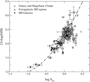
Figure 2.: log S₂₃ vs oxygen abundance.

Another reason why I propose to use this calibration is that, when you use photoionization models with different parameters (and one has to take into account that the highest the metallicity, the more degenerate is the problem), there is no one mechanism that is dominating, none of the three parameters is dominating, so stellar effective temperature, ionization parameter and O abundance, all contribute substantially. When you work with models, you usually get less dispersion with S₂₃ than with R₂₃, maybe because of the lower sensitivity to the electron temperature of the S[III] lines, and perhaps that makes them safe.

One of our questions is if there are people here who have any ideas for other diagnostics, maybe lines in the IR, for high Z regions.

Manuel Peimbert Getting back to what Bernard was saying, I mentioned in my talk that there is already data for about 10 HII regions with recombination lines of O and the point here is that for the 10m telescope of the Canary Islands, it will be important to have a spectrograph of intermediate to high resolution to get these lines, so with a R of 6000 to 9000 I think it will be possible to have hundreds of HII regions with these lines detected, and I think this will improve a lot the calibration. And of course the calibration is needed to use it in objects where we cannot observe these lines. Once it is calibrated, you can go to very high redshifts.

Don Garnett: I would also like to push the IR lines as well, because that will solve a lot of the debate over whether recombination lines or collisionally excited lines give the answer we want. The differences are actually not as large as they seem. What we really need is an independent diagnostic, we need [OIII] 88$\mu$ line measurements and even the mid IR [SIII] will provide a useful diagnostic as well. The answer is Optical/IR comparisons to really push this, to really solve the problem.

Mike Edmunds: OK we are moving along. The new solar O abundance (Allende Prieto et al. 2001). Everybody was a little surprised I think when that went down rather than Orion going up, but there we are. What effect will that have in the global HII region measurements? Bernard, would you like to comment on that?

Bernard Pagel: I was actually rather pleased with this result, because it produced consistency between the Sun and both galactic supergiants and the supergiants in the Magellanic Clouds. I’ve long been maintaining that the chemical evolution of the Magellanic clouds could be understood on the basis of the same yields as the chemical evolution of the local galaxy. So actually I was quite pleased at the new O abundance and what you will also notice is that there is a new C abundance that brings the C/O ratio back to where it was: 8.4 to 8.5 of O and the authors also predict that they are going to bring the N down, so the ratio N/O will be the same. What the rest of the table of abundances shows, without asking you to look in detail at it, is rather a good consistency between stars and HII regions and SNR in the various galaxies of the Local Group, so the upshot of it is, that the HII region abundances remain the same, and the Sun and the stars now finally seem to be catching up with them. But there are implications because all the differencial stellar [O/Fe] abundance analysis that has been done now has to be looked at again, in the light of the new solar O. The obvious reason for this is the blend of the [OI] line with a Ni line, which will have different effect in stars with different metallicity, so that complicates life in some respect.

Rob Kennicutt: I would like to make a very brief comment, and then a question to you Bernard. With Bresolin and Garnett, we are doing an abundance study on M101 (pre-print). We have electron temperatures for 21 HII regions going out from 0.5 to I think 43 Kpc from the centre and we see this offset of about 0.3 dex between the temperature direct abundance forbidden lines ($<t^{2}>$=0 abundances) and the Kewley & Dopita calibrations across the board. In fact in your plot you may have noticed the old Dopita calibration models are quite different from, say what you have done in the past. My question to you relating to that is: the abundances that you have put up, this agreement works if you use $<t^{2}>$=0 classical, auroral line abundances. If in fact those are wrong, due to fluctuations or whatever by a factor of 2, won’t this consistency go away?

Bernard Pagel: That is not quite true. The Orion abundance was based on recombination lines, plus a small correction for O locked on dust grains (Manuel was one of the authors with Esteban et al.). Now the HII region abundances in M31 and M33 were I think largely based on our old R₂₃ method, and so that just leaves the LMC, SMC and NGC6822 OK. Well the implication there is I think that the effective temperature fluctuations are probably not very large. While I’m here I would like to make one other point: I don’t like any attempts at calibrating R₂₃ or any other line-ratio for abundances, based on a sequence of models, partly because the models have inputs like stellar atmospheres and so on as we heard this morning, which are very complicated things, and you can’t always tell what they are going to do, and partly because HII regions don’t necessarily form a smooth sequence. For example Evans and Dopita some time ago assumed a sequence in ionization parameter, and McCall, Ribsky and Shields assumed a sequence in effective temperature, and I don’t think that the HII regions actually know about all that. Further more it’s also a question of regression. When there is a dispersion, a regression of x on y is different from the regression of y on x. And if you are trying to find an abundance then it’s the regression of x on y that you need, not the regression of y on x which people compute from sequences of models. And that’s why I like drawing two straight lines with a corner much better than drawing continuous curves which I think can give very misleading results in certain parts of the diagram.

Elena Terlevich: So, high redshift, use R₂₃? Others? what else would you like? I thought perhaps we could ask Sara Ellison to tell us something about abundances at high redshift. Would you like to? And meanwhile, Gary (Steigman), would you like to ask your question? Or suggest your solution?

Gary Setigman: Well, since I’m only an accompanying spouse naive about the subject, let me ask a naive question. We have O abundances in stars, but we suspect that the abundances on the surface of the Sun are different from the abundances that the Sun started with, and it’s likely that this is true not only for He (which we know from helioseismology) but even for elements like O. So in comparing abundances in stars, don’t we have to worry about the settling of the heavy elements? And for the gas, don’t we have to worry about how much is tied up in dust, and whether it’s the same everywhere in the Universe? I would have thought that the uncertainties are large enough, that any result might be obtained, whether you say that the gas and stars agree or desagree.

Mike Edmunds: On the dust one, I think there is some evidence, which I’ll talk a little bit about on Saturday, that a fairly constant fraction of metals is tied up in dust throughout the Universe - I mean must vary a bit, but constancy may not be too bad an assumption.

Gary Steigman: Do you know the dust is in the same place as the O lines?

Mike Edmunds: No! I’ll shut up at this point.

Bernard Pagel: I just would like to say something regarding the settling. People have thought about the settling quite a lot. And the settling of the He is OK, it’s like about 3 or 4 % and now you’ll notice that I only quoted the abundances to the first decimal, because I found that, you know, quoting the abundances to 2 places of decimals is sort of like a second marriage, a triumph of hope over experience. And my feeling is that in the first place of decimals, the effect of settling in stars like the Sun after convection zones and so on, is probably not something you have to worry about.

Sara Ellison:Last night, Elena actually took advantage of my weakenned state, having just got off an aeroplane after many hours and having had a few sherries, and asked me if I would say something about high redshift abundances. I agreed - that was the effect of the sherry. My own biased view of high redshift abundances means damped Lyman alpha systems. These are the heavy-weight end of the HI column density distribution of quasar absorption line systems. Max Pettini, and I and many others in many countries, have been looking at different abundances in DLA systems. Even though most of what we’ve heard already today has been focused on low z systems, there have been a few DLA abundance results sneaking in there which you might not have noticed. For example: the work that we saw about primordial abundances from Manuel, there were some D results in there that have come from Ly limit systems and DLAs. Also, the work that Gary was showing about the N/O abundances from Max Pettini’s work, this also comes from DLAs. There is a very intimate connection between what we can do with chemical abundances at low and at high redshifts. In essence we are trying to answer the same questions, about the first stages of chemical evolution. I could fill up hours talking about the abundances in DLAs, but I am trying to keep it short, I don’t want to keep you from your “copa de vino”. The advantages that we have when we measure abundances in DLAs are many-fold. For example this whole discussion here about R₂₃ and calibrating the empirical methods, we don’t have to worry about. We can directly determine abundances of many different elements through direct methods, effectively measuring equivalent widths or through fitting Voigt profiles. We can cover dozens of different elements using the rest UV resonant transitions which at high redshift are shifted into the optical, and we immediately have the advantage that we can use ground based telescopes and detectors that are very efficient, whereas people who are studying the local ISM are struggling in the UV. We don’t have to worry very much about ionization corrections, although how much we have to worry about them is still a little bit contentious. One thing we do have to worry about is dust depletion, because we are measuring gas phase abundances, and some relatively unknown fraction of each element is going to be depleted onto dust. So having said all of that, you can really sum up our knowledge of DLA abundances in a nutshell by saying that these are chemically inmature systems. We are seing the first stages of chemical evolution. I noticed that Elena is going to be talking about this “long and arduous search for very metal poor galaxies”; the DLAs are a great test bed for this kind of questions, because they remain metal poor at all z that we have been able to measure so far. The N/O abundances are low, there is no evidence for an enrichment of $\alpha$/Fe peak elements, so all of these are indicators that these are chemically inmature galaxies. I know Elena, Angeles and Mike have circulated a wishlist of what theorists and observers and instrumentalists would like to see coming, or the questions that we would next like to address. Really from the point of view of quasar absorption lines, this is a subject that has really advanced in lockstep with instrumentation. The first big step in terms of results coming from quasar absorption lines came with the introduction of the IPCS, when we could first get good spectra of the quasars and really measure these absorption line systems. The next big advance came with echelle spectrographs on 8m telescopes, so now with instruments like HIRES on Keck and UVES on the VLT, we have got large abundance databases for around 50 to 60 DLAs. I would say we are reaching the limit now of what we can usefully do at that level, and the next instrumentation step I think it has to be made, is actually stepping back from the high resolution point of view. We are using resolution of 40-50000 now, so the next step I think is going to come from turning down the resolution, and turning up the wavelength coverage. We will still need the 8-10m class telescopes, so we can go to much fainter quasars, and we can cover many more lines, and the same lines at different redshifts as well. Keck already has the ESI, and there is talk about a similar, yet more advanced, instrument for VLT. I think this is going to be very important, because at the moment the abundances that we have are very detailed, but of relatively very few systems. Now we are going to increase the number that we have in those databases so we can do complete chemical profiling for many more systems. I also think, in touch with what we have heard today about low redshift systems, making the connection between the high redshift and the low redshift universe is very important, because at the high redshift we are still “shooting blind” - we are not so sure what systems these DLAs represent. We know about their chemistry, but it’s hard to make the link at the moment to the low redshift universe.

Mike Edmunds: Can I comment? There is a problem with the DLA systems. It’s like the old joke about the drunk man looking under the streetlight for the keys he lost elsewhere. We have tended to look where we can see, not where most of the action is happening at high redshift - which in chemical terms is in things such as the forming giant ellipticals. DLAs are a valuable window into this era, but only a partial window.

Sara Ellison: It’s a good point, and that is one of the reasons why I focus on the point that DLAs are good laboratories for metal poor galaxy studies, where you want to ask questions about the EARLY stages of chemical evolution. It’s true that DLAs are probably not representative of the global galaxy population, but is a different line of evidence. It all depends on what question you want to ask. If you want to ask questions about how the N/O ratio is varying in chemically very young galaxies, then DLAs are a good place to look. If you want to know how global metallicity is evolving from redshift 5 to redshift 0, DLAs are probably not the best place to look.

Alec Boksemberg: To follow up very slightly on what was just said about DLA systems, there are other laboratories too, which are pretty good and they are the non-damped systems. It is possible to do quite a lot with those and perhaps they don’t have some of the limitations, for example they may not be so selective, in the sense that they probably don’t have that much dust and they have a broader range of properties. I think the whole combination of absorbers should be looked at, not just selecting particular ones. Although the DLAs are strong objects in attacking the problems, they are not the only ones.

Brian Boyle: I’d like to follow-up on Sara’s comments about instrumentation leading a lot of this. Quite right, but no one has raised the issue of actually looking at a large sample of quasars using the multiobject facilities as are now available in the 8m. The new instrumentation coming along will give you reasonably high resolution over quite wide fields. The quasar surveys now in existence (the 2dF quasar survey, the SLOAN digital sky survey) are now giving the surface density of potential targets to allow you to actually get large number statistics in a wide variety of AGNs, addressing the problem that Alec has just raised here. It is not just the DLA systems that are going to give you answers, but all absorption systems. So I wonder if Sara could comment on the use of those sort of facilities that are coming on line now, to make the next stride forward.

Sara Ellison: It’s a very good point, because we do really need to bump up the statistics. I mentioned about turning down the resolution in order to cover more “objects” (and/or lines) but it’s a fine balance. Using surveys like the 2dF quasar survey and SLOAN is great for pre-selecting your systems. But obviously you cannot study anything like abundances in detail. So I think it’s going to be a very important resource for selecting systems for follow-up with higher resolution instruments which is again going to underline why we need a moderate resolution instrument, because with these very large databases you cannot go through just one per night with UVES.

Claus Leitherer: I would like to add another dimension to the discussion of abundances at high redshift - and that is measurements directly from the stars, because at high redshift we are in the fortunate situation that the rest frame UV is redshifted into the optical. This allows us to define metallicity sensitive indices, pretty much the same as the Lick indices we are all used to, which are mostly sensitive to metallicity and nothing else. Now, from the modelling point of view, this is relatively simple because they come from B stars and there are relatively few uncertainties involved. Now as you can imagine, in terms of observations, a couple of years ago we would have said this is virtually impossible, but now there are some 40 or 50 galaxies available (I am doing this in collaboration with a Cambridge group, Samantha Rix and Max Pettini) where we get a S/N which is sufficient to measure equivalent widths of the order of an Angstrom (which may sound like a lot, but in the UV rest frame it is not a lot). This allows you to compare to models and you can determine abundances to better than a factor of 2, which should be a very useful cross-calibration for comparison with the R23 method.

Elena Terlevich: We would briefly want to touch on two more points that we have been thinking about. Are there any X-ray astronomers prepared to admit they are here? Hagai very kindly has agreed to comment on X-ray abundances.

Hagai Netzer: I’m not going to get you to your wine quickly, I’m afraid! We have heard about galactic wind superbubbles etc, but I think we heard very little about serious attempts to measure the abundance in the observed X-rays. I want to make a couple of points here that I think we should all bear in mind. It’s a very, very difficult job and I must say that NASA, and perhaps to a lesser extent, ESA, are doing a great public relation work in advertising Chandra and XMM-Newton, but most of what has been advertised is based on Chandra’s superb spatial resolution and Newton’s superb (by X-ray standards) spectral resolution. Unfortunately, it’s not really very good for obtaining metallicities from X-ray images of these winds and bubbles because of the S/N: if we want a proper S/N to do it, unfortunately we have to integrate for many hundreds of thousands of seconds. One way I like to think about this is that every second of Chandra time costs about 50 dollars, so you can work out how expensive high S/N observations are. So the result is that what has been published so far (and I want to remind you that these missions are out there for three years already, or at least Chandra is) on X-ray metallicities, is only based on the poor resolution of these spectrographs, because they are using the CCDs. While they improved a lot on the imaging capability, very little has been done on this. So what I want to push for, is to say that if these instruments are being used properly (in the sense that the community decides that it’s worth spending a lot of time on) we should spend a lot of time observing a few - and I mean very very few (it may be 2 or 3 or 4) - of what we all agree, or we should all agree, are standard starburst galaxies. Then we must see emission lines in the X-rays. Individual emission lines have not been observed in these objects, or at least have not been analysed properly. Needless to say, no one can measure the velocity from the X-rays because the resolution is not good enough. So one thing I’m almost tempted to say, and let me finish with that, is that if everybody in this room is willing to sign a petition and the petition will be a proposal for Chandra to spend a million seconds on one object, I think that the entire area of star formation and these bubbles, and what we can learn from the X-rays, will benefit a lot. So far, I don’t think that there is a group of people who were brave enough to propose such long exposures, but this must be done. With present day X-ray instrumentation, the most one can hope for is to obtain good abundance analysis on very few number of objects, ONLY if enough time is spent, and I told you how much time is needed.

Mike Edmunds: So don’t believe all you read about X-ray abundances accurate to less than 0.2 dex! It’s therefore still well worth working on trying to refine optical and infrared metallicity indices.

Angeles Díaz: I will try to end up this discussion by asking all of you: do we believe things like the metallicity vs. luminosity relation for HII galaxies and blue compact galaxies?; do we really believe the shape of the abundance gradients which are being commonly used in chemical evolution models? Until diagnostics are secure, how reliable are all these relations we are talking about?

Mike Edmunds: Probably not in detail! But trends may be OK.

Angeles Díaz: Miguel Mas wants to say one more thing:

Miguel Mas: Yes, I want to give a bit more optimistic view of X-ray spectroscopy than Hagai, in the sense that I agree with him about the data obtained with Chandra. Chandra is very good in its spatial resolution, its spectral resolution is very poor. But on Newton we have a reflection grating spectrometer and this is another story. The data that has been obtained with this RGS on Newton for NGC1068, or NGC253 or for M82, are spectacular, are really splendid. These have not been published until a few months ago and, well, the analysis is really complicated. This is a new tool, a new technique, and what we have to do is to learn how to use this new kind of data which explains why the results have been delayed for two years. But the results are really spectacular. What we are finding is that this hot gas is very metal rich, the amount of metals is solar or over solar by several factors. It seems that we are going in the right direction. And this has been done with 30 kiloseconds integration, which is something acceptable. This will be flying for ten more years. We will have the oportunity to ask for time for very long observations: the tools are there.

Elena Terlevich: Miguel, spectacular plus or minus what?

References

Allende Prieto, C., Lambert, D.L. & Asplund, M. 2001, ApJ, 556, L63

Caplan, J., Deharveng, L., Peña, M., Costero, R. & Blondel, C. 2000, MNRAS, 311, 317

Castellanos, M., Díaz, A.I. & Terlevich, E. 2002, MNRAS, 329, 315

Deharveng, L., Peña, M., Caplan, J. & Costero, R. 2000, MNRAS, 311, 329

Edmunds, M.G. & Pagel, B.E.J. 1984, MNRAS, 211, 507

Kewley, L.J. & Dopita, M.A. 2002, ApJS, 142, 35

Pilyugin, L.S. 2001, A&A, 369,594